High Conductance States in a Mean Field Cortical Network Model

Abstract

Measured responses from visual cortical neurons show that spike times tend to be correlated rather than exactly Poisson distributed. Fano factors vary and are usually greater than 1 due to the tendency of spikes being clustered into bursts. We show that this behavior emerges naturally in a balanced cortical network model with random connectivity and conductance-based synapses. We employ mean field theory with correctly colored noise to describe temporal correlations in the neuronal activity. Our results illuminate the connection between two independent experimental findings: high conductance states of cortical neurons in their natural environment, and variable non-Poissonian spike statistics with Fano factors greater than 1.

1 Introduction

Neurons in primary visual cortex show a large increase in input conductance during visual activation: in vivo recordings (see, e.g., [1]) show that the conductance can rise to more than three times that of the resting state. Such high conductance states lead to faster neuronal dynamics than would be expected from the value of the passive membrane time constant, as pointed out by Shelley et al. [2]. We use mean field theory to study the firing statistics of a model network with balanced excitation and inhibition and observe consistently such high conductance states during stimulation.

In our study, we classify the irregularity of firing with the Fano factor $F$, defined as the ratio of the variance of the spike count to its mean. For temporally uncorrelated spike trains (i.e., Poisson processes) $F=1$, while $F>1$ indicates a tendency for spike clustering (bursts), and $F<1$ points to more regular firing with well separated spikes. Observed Fano factors for spike trains of primary cortical neurons during stimulation are usually greater than 1 and vary within an entire order of magnitude (see, e.g., [3]). We find the same dynamics in our model and are able to pin-point the relevant mechanisms: synaptic filtering leads to spike clustering in states of high conductance (thus $F>1$), and Fano factors depend sensitively on variations in both threshold and synaptic time constants.

2 The Model

We investigate a cortical network model that exhibits self-consistently balanced excitation and inhibition. The model consists of two populations of neurons, an excitatory and an inhibitory one, with dilute random connectivity. The model neurons are governed by leaky integrate-and-fire subthreshold dynamics with conductance-based synapses. The membrane potential of neuron $i$ in population $a$ ($a=1,2$ for excitatory and inhibitory, respectively) obeys

$$\frac{du_{a}^{i}(t)}{dt}=-g_{L}u_{a}^{i}(t)-\sum_{b=0}^{2}\sum_{j=1}^{N_{b}}g_{ab}^{ij}(t)(u_{a}^{i}(t)-V_{b}).$$ (1)

The first sum runs over all populations $b$, including the excitatory input population representing input from the LGN and indexed by $0$. The second sum runs over all neurons $j$ in population $b$ of size $N_{b}$. The reversal potential $V_{b}$ for the excitatory inputs ($b=0,1$) is higher than the firing threshold, the one for the inhibitory inputs ($V_{2}$) is below the reset value. The constant leakage conductance $g_{L}$ is the inverse of the membrane time constant $\tau_{m}$.

The time dependent conductance $g_{ab}^{ij}(t)$ from neuron $j$ in population $b$ to neuron $i$ in population $a$ is taken as

$$g_{ab}^{ij}(t)=\frac{g_{ab}^{0}}{\sqrt{K_{b}}}\sum_{s}\exp(-(t-t^{j}_{s})/\tau_{b})\Theta(t-t^{j}_{s})$$ (2)

if there is a connection between those two neurons, otherwise zero. The sum runs over all spikes $s$ emitted by neuron $j$, $\tau_{b}$ is the synaptic time constant for the synapse of type $b$ (excitatory or inhibitory), and $\Theta$ is the Heavyside step function. $K_{b}$ denotes the average number of presynaptic neurons in population $b$. We followed van Vreeswijk and Sompolinsky [4] by scaling the conductances with $1/\sqrt{K_{b}}$ so that their fluctuations are of order one, independent of network size.

3 Mean Field Theory

We use mean field theory to reduce the full network problem to two neurons: one for each population. This method is exact in the limit of large populations with homogeneous connection probabilities [5]. The neurons receive self-consistent inputs from their cortical environment, exploiting the fact that all neurons within a population exhibit the same firing statistics due to homogeneity. The time dependent conductance described in (2) can then be replaced by a realization of a Gaussian distributed random variable $g_{ab}$ with mean

$$\langle g_{ab}\rangle=g_{ab}^{0}\sqrt{K_{b}}\,r_{b},$$ (3)

and covariance

$$\langle\delta g_{ab}(t)\,\delta g_{ab}(t^{\prime})\rangle=(g_{ab}^{0})^{2}(1-K_{b}/N_{b})\,C_{b}(t-t^{\prime}),$$ (4)

Here, $r_{b}$ is the firing rate of the presynaptic neuron $b$, and $C_{b}(t-t^{\prime})$ is the autocorrelation function of its spike train. A simple approximation of the autocorrelation, like the one used by [6] and [7], is to assume $g_{ab}(t)$ to be temporally uncorrelated (i.e., white noise), in which case it simplifies to $C_{b}(t-t^{\prime})=r_{b}\,\delta(t-t^{\prime})$. The term $(1-K_{b}/N_{b})$ is a correction for the finite connection concentration $K_{b}/N_{b}$ and can be derived using the methods of [8].

The self-consistent balance condition is obtained by setting the net current in (1) to zero when the membrane potential is at threshold $\theta_{a}$ and the conductances have their mean values (3). In the large $K_{b}$-limit, it reads

$$\sum_{b=0}^{2}g_{ab}^{0}\sqrt{K_{b}}\,r_{b}\,(\theta_{a}-V_{b})=0.$$ (5)

The distribution of the variables $g_{ab}$ can be calculated numerically using an iterative approach [9]. One starts with a guess based on the balance equation (5) for the means and covariances and generates a large sample of specific realizations of $g_{ab}(t)$, which are used to integrate (1) to generate a large sample of spike trains. The latter can then be used to calculate new estimates of the means and covariances by applying (3) and (4) and correction of the initial guess towards the new values. These steps are repeated until convergence.

4 Results

For the above described model, we chose parameters corresponding to population sizes of 16,000 excitatory neurons and 4,000 inhibitory neurons, representing a small patch of layer IV cat visual cortex. The neurons were connected randomly, with 10% connection probability between any two neurons. The firing threshold was fixed to 1, excitatory and inhibitory reversal potentials were set to $+14/3$ and $-2/3$, respectively, and the membrane time constant $\tau_{m}=g_{L}^{-1}$ was $10$ ms. For the results presented here, the integration time step was 0.5 ms.

Figure 1 illustrates the importance of coloring the noise produced by intra-cortical activity. The white noise approximation underestimates both the correlation times and the strength of the correlations in the neuron’s firing: its autocorrelation (blue) is both narrower and weaker than the one for colored noise (red).

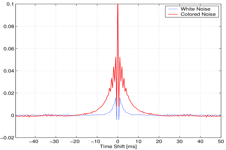
Figure 1: Autocorrelation functions for white noise (blue) and colored noise (red). The white noise approximation underestimates the amount of temporal correlation in the neuron’s firing.

Fano factors vary systematically with both the distance between reset and threshold and the synaptic time constant $\tau_{s}$. Non-zero synaptic time constants produced consistently Fano factors greater than one. We varied the reset between 0.8 and 0.94 and $\tau_{s}$ between 0 and 6 ms, which resulted in values for $F$ that span an entire order of magnitude, from slightly above 1 to approximately 10 for $\tau_{s}\geq 2$ ms (see Figure 2).

Figure 2: Fano factors for a range of reset values and synaptic time constants $\tau_{s}$. Longer synaptic time constants lead to increased clustering (bursts) of spikes, which is reflected in higher Fano factors.

5 Discussion

In all our simulations, we observed that the membrane potential changed on a considerably faster time scale than the membrane time constant $\tau_{m}=10$ ms. This behavior is only observed if conductance-based synapses are included in the integrate-and-fire neuron model. To understand this phenomenon, it is convenient to follow the notation of Shelley et al. [2] to rewrite the equation for the membrane potential dynamics (1) in the following form:

$$\frac{du_{a}(t)}{dt}=-g_{T}(t)\left(u_{a}(t)-V_{S}(t)\right),$$ (6)

with the total conductance $g_{T}(t)=g_{L}+\sum_{b}g_{ab}(t)$, and the effective reversal potential $V_{S}(t)=g_{T}(t)^{-1}\sum_{b}g_{ab}(t)V_{b}$. The membrane potential $u_{a}(t)$ follows the effective reversal potential with the input dependent effective membrane time constant $g_{T}(t)^{-1}$. The effective reversal potential changes on the time scale of the synaptic time constants, which are up to five times shorter than $\tau_{m}$ in our simulations. However, if the effective membrane time constant is shorter than the synaptic time constant due to a large enough total conductance, then $u_{a}(t)$ can follow $V_{S}(t)$ closely, as observed in our simulations (see Figure 3).

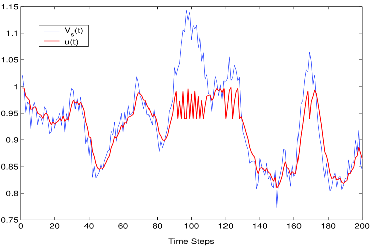
Figure 3: The membrane potential $u(t)$ (red) follows the effective reversal potential $V_{S}(t)$ (blue) closely, except for detours when the neuron is reset due to firing. The membrane potential recovers fast enough to spike several times while $V_{S}(t)$ stays above threshold, thus producing bursts of spikes. Here, the threshold is set to 1 and the reset to 0.94.

In high conductance states, the firing statistics are strongly influenced by synaptic dynamics (see Figure 2). This is in contrast with strictly current based models, where the neuron reacts too slow to reflect fast synaptic dynamics in its firing. The ‘synaptic filtering’ of arriving spikes leads to temporal correlations in $V_{S}(t)$ and thus to temporal correlations (by way of spike clustering) in firing. Therefore, the model neurons receive temporally correlated input rather than white noise. For this reason, in mean field models dealing with conductance based dynamics, coloring the noise is important to arrive at the full amount of temporal correlation in firing statistics (see Figure 1). We confirmed these considerations by running simulations without synaptic filtering ($\tau_{s}=0$). As expected, intra-cortical activity became uncorrelated and the white noise approximation produced the same result as coloring the noise correctly. In that case, Fano factors stayed close to 1 (see Figure 2), i.e, no tendency of spike clustering was observed.

Previous investigations showed that varying the distance between threshold and reset in balanced integrate-and-fire networks has a strong effect on the irregularity of the firing [10]. By including a conductance-based description of synapses, we were now able to show the importance of synaptic time constants on firing statistics, even if they are several times smaller than the passive membrane time constant: Synaptic filtering facilitates clustering of spikes in states of high conductance.

References

- [1] L J Borg-Graham, C Monier, and Y Fregnac, Nature 393:369-374 (1998).
- [2] M Shelley, D McLaughlin, R Shapley, and J Wielaard, J. Comput. Neurosci, 13:93-109 (2002).
- [3] E D Gershon, M C Wiener, P E Latham and B J Richmond, J Neurophysiol 79:1135-1144 (1998).
- [4] C van Vreeswijk and H Sompolinsky, Science 274:1724-1726 (1996), Neural Comp 10:1321-1371 (1998).
- [5] C Fulvi Mari, Phys Rev Lett 85:210-213 (2000).
- [6] D J Amit and N Brunel, Cerebral Cortex 7:237-252 (1997).
- [7] N Brunel, J Comput Neurosci 8:183-208 (2000).
- [8] R Kree and A Zippelius, Phys Rev A 36:4421-4427 (1987).
- [9] H Eisfeller and M Opper, Phys Rev Lett 68:2094-2097 (1992)
- [10] J Hertz, B J Richmond, and K Nilsen, CNS 2002, to be published in Neurocomputing (2003).