Discriminative Topological Features Reveal Biological Network Mechanisms

Abstract

Recent genomic and bioinformatic advances have motivated the development of numerous random network models purporting to describe graphs of biological, technological, and sociological origin. The success of a model has been evaluated by how well it reproduces a few key features of the real-world data, such as degree distributions, mean geodesic lengths, and clustering coefficients. Often pairs of models can reproduce these features with indistinguishable fidelity despite being generated by vastly different mechanisms. In such cases, these few target features are insufficient to distinguish which of the different models best describes real world networks of interest; moreover, it is not clear a priori that any of the presently-existing algorithms for network generation offers a predictive description of the networks inspiring them. To derive discriminative classifiers, we construct a mapping from the set of all graphs to a high-dimensional (in principle infinite-dimensional) “word space.” This map defines an input space for classification schemes which allow us for the first time to state unambiguously which models are most descriptive of the networks they purport to describe. Our training sets include networks generated from 17 models either drawn from the literature or introduced in this work, source code for which is freely available [1]. We anticipate that this new approach to network analysis will be of broad impact to a number of communities.

1 Introduction

The post-genomic revolution has ushered in an ensemble of novel crises and opportunities in rethinking molecular biology. The two principal directions in genomics, sequencing and transcriptome studies, have brought to light a number of new questions and forced the development of numerous computational and mathematical tools for their resolution. The sequencing of whole organisms, including homo sapiens, has shown that in fact there are roughly the same number of genes in men and in mice. Moreover, much of the coding regions of the chromosomes (the subsequences which are directly translated into proteins) are highly homologous. The complexity comes then, not from a larger number of parts, or more complex parts, but rather through the complexity of their interactions and interconnections.

Coincident with this biological revolution – the massive and unprecedented volume of biological data – has blossomed a technological revolution with the popularization and resulting exponential growth of the Internet. Researchers studying the topology of the Internet [2] and the World Wide Web [3] attempted to summarize their topologies via statistical quantities, primarily the distribution $P(k)$ over nodes of given connectivity or degree $k$, which it was found, was completely unlike that of a “random” or Erdos-Renyi graph . Instead, the distribution obeyed a power-law $P(k)\sim k^{-\gamma}$ for large $k$. This observation created a flurry of activity among mathematicians at the turn of the millennium both in (i) measuring the degree distributions of innumerable technological, sociological, and biological graphs (which generically, it turned out, obeyed such power-law distributions) and (ii) proposing myriad models of randomly-generated graph topologies which mimicked these degree distributions (cf. [6] for a thorough review). The success of these latter efforts reveals a conundrum for mathematical modeling: a metric which is universal (rather than discriminative) cannot be used for choosing the model which best describes a network of interest. The question posed is one of classification, meaning the construction of an algorithm, based on training data from multiple classes, which can place data of interest within one of the classes with small test loss.

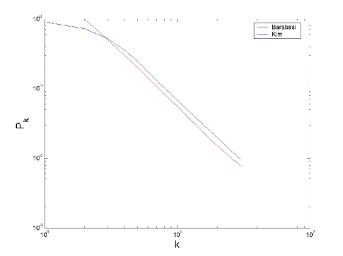
Figure 1: Ambiguity in network mechanisms: we plot the degree distribution of two graphs generated using radically different algorithms. The red line results from an algorithm of the Barabasi class [3]; the blue from the “static” model of Kim et al [8]. The distributions are indistinguishable, illustrating the insufficiency of degree distributions as a classifying metric.

In this paper, we present a natural mapping from a graph to an infinite-dimensional vector space using simple operations on the adjacency matrix. We then test a number of different classification (including density estimation) algorithms which prove to be effective in finding new metrics for classifying real world data sets. We selected 17 different models proposed in the literature to model various properties of naturally occurring networks. Among them are various biologically inspired graph-generating algorithms which were put forward to model genetic or protein interaction networks. To assess their value as models of their intended referent, we classify data sets for the E. coli genetic network, the C. elegans neural network and the yeast S. cerevisiae protein interaction network. We anticipate that this new approach will provide a general tool of analysis and classification in a broad diversity of communities.

The input space used for classifying graphs was introduced in our earlier work [9] as a technique for finding statistically significant features and subgraphs in naturally occurring biological and technological networks. Given the adjacency matrix $A$ representing a graph (i.e., $A_{ij}=1$ iff there exists an edge from $j$ to $i$), multiplications of the matrix count the number of walks from one node to another (i.e., $[A^{n}]_{ij}$ is the number of unique walks from $j$ to $i$ in $n$ steps). Note that the adjacency matrix of an undirected graph is symmetric. The topological structure of a network is characterized by the number of open and closed walks of given length. Those can be found by calculating the diagonal or non-diagonal components of the matrix, respectively. For this we define the projection operation $D$ such that

$$[D(A)]_{ij}=A_{ij}\delta_{ij}$$ (1)

and its complement $U=I-D$. (Note that we do not use Einstein’s summation convention. Indices $i$ and $j$ are not summed over.) We define the primitive alphabet $\{A;T,U,D\}$ as the adjacency matrix $A$ and the operations $T,U,D$ with the transpose operation $T(A)\equiv A^{T}$ distingushing walks “up” the graph from walks ”down” the graph. From the letters of this alphabet we can construct words (a series of operations) of arbitrary length. A number of redundancies and trivial cases can be eliminated (for example, the projection operations satisfy $DU=UD=0$) leading to the operational alphabet $\{A,AT,AU,AD,AUT\}$. The resulting word is a matrix representing a set of possible walks generated by the original graph. An example is shown in Figure 2.

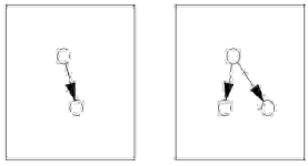
Figure 2: The elements of the matrix $ATA$ count these two walks. $TA$ corresponds to one step “up” the graph, the following $A$ to one step “down”. The last node could be either the same as the starting node as in the first subgraph (accounted for by the diagonal part $DATA$) or a different node as in the second subgraph (accounted for by the non-diagonal part $UATA$).

Each word determines two relevant statistics of the network: the number of distinct walks and the number of distinct pairs of endpoints. These two statistics are determined by either summing the entries of the matrix (sum) or counting the number of nonzero elements (nnz) of the matrix, respectively. Thus the two operations sum and nnz map words to integers. This allows us to plot any graph in a high-dimensional data space: the coordinates are the integers resulting from these path-based functionals of the graph’s adjacency matrix.

The coordinates of the infinite-dimensional data space are given by integer-valued functionals

$$F(L_{1}L_{2}\dots L_{n}A)$$ (2)

where each $L_{i}$ is a letter of the operational alphabet and $F$ is an operator from the set $\{{\texttt{sum}},{\texttt{sum}}D,$ ${\texttt{sum}}U,{\texttt{nnz}},{\texttt{nnz}}D,{\texttt{nnz}}U\}$. We found it necessary only to evaluate words with $n\leq 4$ (counting all walks up to length 5) to construct low test-loss classifiers. Therefore, our word space is a $6\sum_{i=1}^{4}{5^{i}}=4680$-dimensional vector space, but since the words are not linearly independent (e.g., ${\texttt{sum}}U+{\texttt{sum}}D={\texttt{sum}}$), the dimensionality of the manifold explored is actually much smaller. However, we continue to use the full data space since a particular word, though it may be expressed as a linear combination of other words, may be a better discriminator than any of its summands.

In [9], we discuss several possible interpretations of words, motivated by algorithms for finding subgraphs. Previously studied metrics can sometimes be interpreted in the context of words. For example, the transitivity of a network can be defined as 3 times the number of 3-cycles divided by the number of pairs of edges that are incident on a common vertex. For a loopless graph (without self-interactions), this can also be calculated as a simple expression in word space: ${{\texttt{sum}}(DAAA)}/{{\texttt{sum}}(UAA)}$. Note that this expression of transitivity as the quotient of two words implies separation in two dimensions rather than in one. However, there are limitations to word space. For example, a similar measure, the clustering coefficient, defined as the average over all vertices of the number of 3-cycles containing the vertex divided by the number of paths of length two centered at that vertex, cannot be easily expressed in word space because vertices must be considered individually to compute this quantity. Of course, the utility of word space is not that it encompasses previously studied metrics, but that it can elucidate new metrics in an unbiased, systematic way, as illustrated below.

2 Classification Methods

2.1 SVMs

A standard classification algorithm which has been used with great success in myriad fields is the support vector machine, or SVM [10]. This technique constructs a hyperplane in a high-dimensional feature space separating two classes from each other. Linear kernels are used for the analysis presented here; extensions to appropriate nonlinear kernels are possible.

We rely on a freely available C-implementation of SVM-Light [11], which uses a working set selection method to solve the convex programming problem with Lagrangian

$$L({\mathbf{w}},b)=\frac{1}{2}|{\mathbf{w}}|^{2}-C\sum_{i=1}^{m}{\xi_{i}}$$ (3)

with $y_{i}({\mathbf{w}}\cdot{\bf x}_{i}+b)\geq 1-\xi_{i};i=1,\dots,m$ where $f({\bf x})={\bf{w}}\cdot{\bf x}+b$ is the equation of the hyperplane, ${\bf x}_{i}$ are training examples and $y_{i}\in\{-1,+1\}$ their class labels. Here, $C$ is a fixed parameter determining the trade-off between small errors $\xi_{i}$ and a large margin ${2}/{|{\mathbf{w}}|}$. We set $C$ to a default value $(\frac{1}{m}\sum_{i=1}^{m}{{\bf x}_{i}^{2}})^{-1}$. We observe that training and test losses have a negligible dependence on $C$ since most test losses are near or equal to zero even in low-dimensional projections of the data space.

2.2 Robustness

Our objective is to determine which of a set of proposed models most accurately describes a given real data set. After constructing a classifier enjoying low test loss, we classify our given real data set to find a ‘best’ model. However, the real network may lie outside of any of the sampled distributions of the proposed models in word space. In this case we interpret our classification as a prediction of the least erroneous model.

We distinguish between the two cases by noting the following: Consider building a classifier for apples and grapefruit which is then faced with an orange. The classifier may then decide that, based on the feature size the orange is an apple. However, based on the feature taste the orange is classified as a grapefruit. That is, if we train our classifier on different subsets of words and always get the same prediction, the given real network must come closest to the predicted class based on any given choice of features we might look at. We therefore define a robust classifier as one which consistently classifies a test datum in the same class, irrespective of the subset of features chosen. And we measure robustness as the ratio of the number of consistent predictions over the total number of subspace-classifications.

2.3 Generative Classifiers

A generative model, in which one infers the distribution from which observations are drawn, allows a quantitative measure of model assignment: the probability of observing a given word-value given the model. For a robust classifier, in which assignment is not sensitively dependent on the set of features chosen, the conditional probabilities should consistently be greatest for one class.

We perform density estimations with Gaussian kernels for each individual word, allowing calculation of $p(C=c|X_{j}=x)$, the probability of being assigned to class $c$ given a particular value $x$ of word $j$. By comparing ratios of likelihood values among the different models, it is therefore possible, for the case of non-robust classifiers, to determine which of the features of an orange come closest to an apple and which features come closest to a grapefruit.

We compute the estimated density at a word value $x_{0}$ from the training data $x_{i}$ ($i=1,\dots,m$) as

$$p(x_{0},\lambda)=\frac{1}{m(2\lambda^{2}\pi)^{1/2}}\sum_{i=1}^{m}{e^{-\frac{1}{2}(|x_{i}-x_{0}|/\lambda)^{2}}}$$ (4)

where we optimize the smoothing parameter $\lambda$ by maximizing the probability of a hold-out set using 5-fold cross-validation. More precisely, we partition the training examples into 5-folds $F_{i}=\{x_{f_{i}(j)}\}_{j=1\dots N_{i}}$, where $f_{i}$ is the set of indices associated with fold $i$ ($i=1\dots 5$) and $N_{i}=card(F_{i})$. We then maximize

$$Q(\lambda)=\frac{1}{5}\sum_{i=1}^{5}\sum_{j=1}^{N_{i}}{\log{p(x_{f_{i}(j)},\lambda)}}$$ (5)

as a function of $\lambda$. In all cases we found that $Q(\lambda)$ had a well pronounced maximum as long as the data was not oversampled. Because words can only take integer values, too many training examples can lead to the situation that the data take exactly the same values with or without the hold-out set. In this case, maximizing $Q(\lambda)$ corresponds to $p(x,\lambda)$ having single peaks around the integer values, so that $\lambda$ tends to zero. Therefore, we restrict the number of training examples to $4N_{v}$, where $N_{v}$ is the number of unique integer values taken by the training set. With this restriction $Q(\lambda)$ showed a well-pronounced maximum at a non-zero $\lambda$ for all words and models.

2.4 Word Ranking and Decision Trees

The simplest scheme to find new metrics which can distinguish among given models is to take a large number of training examples for a pair of network models and find the optimal split between both classes for every word separately. We then test every one-dimensional classifier on a hold-out set and rank words by lowest test loss. Below we show that this simple approach is already very successful.

Extending these results, one can ask how many words one needs to distinguish entire sets of different models, as estimated by building a multi-class decision tree and measuring its test loss for different numbers of terminal nodes. We use Matlab’s Statistical Toolbox with a binary multi-class cost function to decide the splitting at each node. To avoid over-fitting the data, we prune trained trees and select the subtree with minimal test loss by 10-fold cross-validation.

Additionally, we propose a different approach using decision trees to find most discriminative words. For every possible model pair $(i,j)$ for $1\leq i<j\leq N_{mod}$ where $N_{mod}$ is the total number of models, we build a binary decision tree, but restricted so that at every level of each tree the same word has to be used for all the trees. At every level the best word is chosen according to the smallest average training loss over all binary trees. The model is not meant to be a substitution to an ordinary multi-class decision tree. It merely represents another algorithm which may be useful to find a fixed number of most discriminative words, for example for visualization of the distributions in a three-dimensional subspace.

3 Network Models

We sample training data for undirected graphs from six growth models, one scale-free static model [12][8][13], the Small World model [14], and the Erdös-Rényi model [15]. Among the six growth models two are based on preferential attachment [16][7], three on a duplication-mutation mechanism [17][18], and one on purely random growth [19]. For directed graphs we similarly train on two preferential attachment models [20], two static models [21][22][8], three duplication-mutation models [23][24], and the directed Erdös-Rényi model [15]. More detailed descriptions and source code are available on our website [1].

In order to classify real data, we sample training examples of the given models with a fixed total number of nodes $N_{0}$, and allow a small interval $I_{M}$ of 1-2% around the total number of edges $M_{0}$ of the considered real data set. All additional model parameters are sampled uniformly over a given range which is specifid by the model’s creators in most cases, otherwise can be given reasonable bounds. Such a generated graph is accepted if the number of edges $M$ falls into the specified interval $I_{M}$ around $M_{0}$, thereby creating a distribution of graphs associated to each model which could describe the real data set with given $N_{0}$ and $M_{0}$.

4 Results

We apply our methods to three different real data sets: the E. coli genetic network [25](directed), the S. cerevisiae protein interaction network [26](undirected), and the C. elegans neural network [27](directed).

Each node in E. coli’s genetic network represents an operon coding for a putative transcriptional factor. An edge exists from operon $i$ to operon $j$ if operon $i$ directly regulates $j$ by binding to its operator site. This gives a very sparse adjacency matrix with a total of 423 nodes and 519 edges.

The S. cerevisiae protein interaction network has 2114 nodes and 2203 undirected edges. Its sparseness is therefore comparable to E. coli’s genetic network.

The C. elegans data set represents the organism’s fully mapped neural network. Here, each node is a neuron and each edge between two nodes represents a functional, directed connection between two neurons. The network consists of 306 neurons and 2359 edges, and is therefore about 7 times more dense than the other two networks.

We create training data for undirected or directed models according to the real data set. All parameters other than the numbers of nodes and edges were drawn from a uniform distribution over their range. We sampled 1000 examples per model for each real data set, trained a pairwise multi-class SVM on 4/5 of the sampled data and tested on the 1/5 hold-out set. We determine a prediction by counting votes for the different classes. Table 1 summarizes the main results.

	E. coli	C. elegans	S. cerevisiae
$\langle L_{tr}\rangle$	$1.6\%$	$0.5\%$	$2.1\%$
$\langle L_{tst}\rangle$	$1.6\%$	$0.5\%$	$1.8\%$
$\langle N_{sv}\rangle$	109	51	106
Winner	Kumar	MZ	Sole
Robustness	1.0	.97	0.64

Table 1: Results of multi-class SVM. $\langle L_{tr}\rangle$ is the empirical training loss averaged over all pairwise classifiers, $\langle L_{tst}\rangle$ is the averaged empirical test loss. $\langle N_{sv}\rangle$ is the average number of support vectors. The winner is the model that got the highest number of votes when classifying the given real data set.

All three classifiers show very low test loss and two of them a very high robustness. The average number of support vectors is relatively small. Indeed, some pairwise classifiers had as few as three support vectors and more than half of them had zero test loss. All of this suggests the existence of a small subset of words which can distinguish among most of these models.

The predicted models Kumar, MZ, and Sole are based on very similar mechanisms of duplication and mutation. The model by Kumar et al was originally meant to explain various properties of the WWW. It is based on a duplication mechanism, where at every time step a prototype for the newly introduced node is chosen at random, and connected to the prototype’s neighbors or other randomly chosen nodes with probability $p$. It is therefore built on an imperfect copying mechanism which can also be interpreted as duplication-mutation, often evoked when considering genetic and protein-interaction networks. Sole is based on the same idea, but allows two free parameters, a probability controlling the number of edges copied and a probability controlling the number of random edges created. MZ is essentially a directed version of Sole. Moreover, we observe that none of the preferential attachment models came close to being a predicted model for one of our biological networks even though they, and other preferential attachment models in the literature, were created to explain power-law degree distributions. The duplication-mutation scheme arises as the more successful one.

Kumar and MZ were classified with almost perfect robustness against 500-dimensional subspace sampling. With 26 different choices of subspaces, E. coli was always classified as Kumar. We therefore assess with high confidence that Kumar and MZ come closest to modeling E. coli and C. elegans, respectively. In the case of Sole and the S. cerevisiae protein network we observed fluctuations in the assignment to the best model. 3 out of 22 times S. cerevisiae was classified as Vazquez (duplication-mutation) , other times as Barabasi (preferential attachment), Klemm (duplication-mutation), Kim (scale-free static) or Flammini (duplication-mutation) depending on the subset of words chosen. This clearly indicates that different features support different models. Therefore the confidence in classifying S. cerevisiae to be Sole is limited.

Figure 3: Kernel Density Estimation of nnz $D(AUTAUTAUAUTA)$ for two models of E. coli (Kumar and Krapivsky-Bianconi). Log-Likelihoods: $\log(p_{kumar})=-4.22,\log(p_{krap-bianc})=-12.0$.

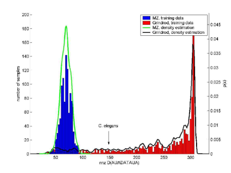
Figure 4: Kernel Density Estimation of nnz $D(AUADATAUA)$ for two top- scoring models of C. elegans (Middendorf-Ziv and Grindrod). Log-Likelihoods: $\log(p_{mz})=-376,\log(p_{grind})=-6.23$.

The preference of individual words for individual models is investigated using kernel density estimation 2.3 by finding words which maximize $p_{i}(x_{0})/p_{j}(x_{0})$ for two different models ($i$ and $j$) at a word value of the real data set $x_{0}$. Figure 4 shows the sampled distribution and estimated density for the word which extremely disfavors the winning model over its follower. The opposite case is shown in 3 for E. coli, where the word supports the winning model and disfavors its follower. More specifically we are able to verify that most of the words of E. coli are most likely to be generated by Kumar. Indeed, out of 1897 words taking at least 2 integer values for all of the models (density estimation for a single value is not meaningful), the estimated density at the E. coli word value was highest for Kumar in 1297 cases, for Krapivsky-Bianconi in 535 cases and for Krapivsky in only 65 cases.

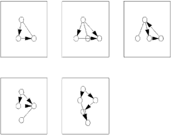
Figure 5: Subgraphs associated with the word nnz$DAUTAUTAUAUTA$. The word has a non-zero value iff at least one of these subgraphs occurs in the network

Figure 3 shows the distributions for the word nnz$DAUTAUTAUAUTA$ which had a maximum ratio of probability density of Kumar over the one of Krapivsky-Bianconi at the E. coli position. E. coli in fact has a zero word count meaning that none of the associated subgraphs shown in Figure 5 actually occur in E. coli. Four of those subgraphs have a mutual edge which is absent in the E. coli network and also impossible to generate in a Kumar graph. Krapivsky-Bianconi graphs allow for mutual edges which could be one of the reasons for a higher count in this word. Another source might be that the fifth subgraph showing a higher order feed-forward loop is more probable to be generated in a Krapivsky-Bianconi graph than in a Kumar graph. This subgraph also has to be absent in the E. coli network since it gives a zero word value, showing that the Kumar and the Krapivsky-Bianconi models have both a tendence to give rise to a topological structure that does not exist in E. coli. This analysis gives an example of how these findings are useful in refining network models and in deepening our understanding of real networks. For further discussions refer to our website [1]

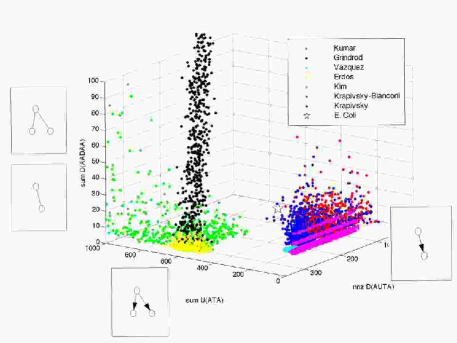
Figure 6: E. coli and seven directed models. The distributions in word space are shown for a projection onto the subspace of the three most discriminatve words. Subgraphs associated with every word are also shown.

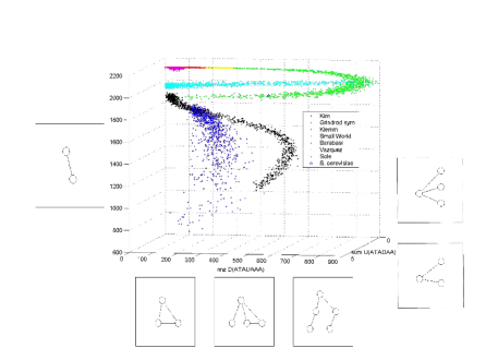
Figure 7: S. cerevisiae and 7 undirected models. The distributions in word space are shown for a projection onto the subspace of the three most discriminative words. Subgraphs associated with every word are also shown.

The SVM results suggest that one may only need a small subset of words to be able to separate most of the models with almost zero test loss. The simplest approach to find such a subset is to look at every word for a given pair of models and compute the best split, then ranking words by lowest training loss. We find that among the most discriminative words some occur very often such as nnz$AA$ or nnz$ATA$, which count the pairs of edges attached to the same vertex and either pointing in the same direction or pointing away from each other, respectively. Other frequent words include nnz$DAA$, nnz$DATA$ and sum$UATA$. A striking feature of this single-word analysis is that the test loss associated with simple one-dimensional classifiers are comparable to the SVM test loss confirming that most pairs of models are separable with only a few words. To consider all of the models at once and not just in pairs we apply both tree algorithms described in 2.4 to all three data sets. Figures 6 and 7 show scatter-plots of the training data using the most discriminative three words. Taking those three words the average training-loss over all pairs of models is 1.7%, 0.8% and 0.2% for the E. coli, C. elegans and S. cerevisiae training data, respectively.

5 Conclusions

It is not surprising that models with different mechanisms are distinguishable; however, the fact that these models have not been separated in a systematic manner to date points to the inadequacy of current metrics popular in the network theory community. We have shown that a systematic enumeration of countably infinite features of graphs can be successfully used to find new metrics which are highly efficient in separating various kinds of models. Furthermore, they allow us to define a high-dimensional input space for classification algorithms which for the first time are able to decide which of a given set of models most accurately describes three exemplary biological networks.

6 Acknowledgments

It is a pleasure to acknowledge useful conversations with C. Leslie, D. Watts, and P. Ginsparg. We also acknowledge the generous support of NSF VIGRE grant DMS-98-10750, NSF ECS-03-32479, and the organizers of the LANL CNLS 2003 meeting and the COSIN midterm meeting 2003.

Appendix A Supplementary tables

Name	Fundamental Mechanism	References
Bianconi	Growth model with a probability of attaching to an existing node $p\sim\eta_{i}k_{i}$, where $\eta_{i}$ is a fitness parameter. Here we use a random fitness landscape, where $\eta$ is drawn from a uniform distribution in $(0,1)$	[16]
Callaway	Growth model adding one node and several edges between randomly chosen existing nodes (not necessarily the newly introduced one) at every time step.	[19]
Kim	A “static” model giving rise to a scale-free network. Edges are created between nodes chosen with a probability $p\sim i^{-\alpha}$ where $i$ is the label of the node and $\alpha$ a constant parameter in $(0,1)$.	[12],[8],[13]
Erdos	Undirected random graph.	[15]
Flammini	Growing graph based on duplication modeling protein interactions. At every time step a prototype is chosen randomly. With probability $q$ edges of the prototype are copied. With probability $p$ an edge to the prototype is created.	[17]
Klemm	Growing graph using sets of active and inactive nodes to model citation networks.	[30], [31]
Small World	Interpolation between a regular lattice and a random graph. We replace edges in the regular lattice by random ones.	[14]
Barabasi	Growing graph with a probability of attaching to an existing node $p\sim k_{i}$. (“Bianconi” with $\eta_{i}=1$ for all $i$)	[7]
Sole	Growing graph initialized with a 5-ring substrate. At every time step a new node is added and a prototype is chosen at random. The prototype’s edges are copied with a probability $p$. Furthermore, random nodes are connected to the newly introduced node with probability $q/N$, where $p$ and $q$ are given parameters in $(0,1)$ and $N$ is the number of total nodes at the considered time step.	[18]

Table 2: Undirected Network Models. $k_{i}$ is the degree of the $i$-th node.

Name	Fundamental Mechanism	References
Kim	Directed version of “Kim”. A “static” model giving rise to a scale-free network. Edges are created between nodes chosen with probabilites $p\sim i^{\alpha}_{in}$ and $q\sim j^{\alpha}_{out}$ where $\alpha_{in}$ and $\alpha_{out}$ are fixed parameters chosen in $(0,1)$ and $i$($j$) is the label of the $i$-th ($j$-th) node	[8]
Erdos	Directed random graph.	[15]
Grindrod	Static graph. Edges are created between nodes $i$, $j$ with probability $p=b\lambda^{|i-j|}$, where $b$ and $\lambda$ are fixed parameters.	[22],[21]
Krapivksy	Growing graph modeling the WWW. At every time step either a new edge, or a new node with an edge, are created. Nodes to connect are chosen with probability $p\sim k_{i,in}+a$ and $q\sim k_{j,out}+b$ based on preferential attachment with fixed real-valued offsets $a$ and $b$.	[20]
Krapivsky-Bianconi	Extension of “Krapivsky” using a random fitness landscape multiplying the probabilities for preferential attachment. It is the directed analog of “Bianconi” being an extension to “Barabasi”.	(original)
Kumar	Growing graph based on a copying mechanism to model the WWW. At every time step a prototype $P$ is chosen at random. Then for every edge connected to $P$, with probability $p$ an edge between the newly introduced node and $P$’s neighbor is created, and with probability $(1-p)$ an edge between the new node and a randomly chosen other node is created.	[23]
Middendorf-Ziv (MZ)	Growing directed graph modeling biological network dynamics. A prototype is chosen at random and duplicated. The prototype or progenitor node has edges pruned with probability $\beta$ and edges added with probability $\alpha\ll\beta$. Based loosely on the undirected protein network model of Sole et al. [18].	original
Vazquez	Growth model based on a recursive ‘copying’ mechanism, continuing to 2nd nearest neighbors, 3rd nearest neighbors etc. The authors call it a ‘random walk’ mechanism.	[24]

Table 3: Directed Network Models. $k_{i,in}$ ($k_{i,out}$) is the in-(out-)degree of the $i$-th node.

	votes	Kumar	Krapivsky-Bianconi	Krapivsky	Kim	Vazquez	Erdos	Grindrod	MZ
Kumar	7/7		$f({\bf x})=1.48$	$f({\bf x})=2.32$	$f({\bf x})=2.80$	$f({\bf x})=1.12$	$f({\bf x})=3.58$	$f({\bf x})=3.11$	$f({\bf x})=1.26$
			$L_{tst}=5.3$%	$L_{tst}=4.5$%	$L_{tst}=0.8$%	$L_{tst}=0.0$%	$L_{tst}=0.0$%	$L_{tst}=0.0$%	$L_{tst}=0.0$%
			$L_{tr}=4.4$%	$L_{tr}=3.2$%	$L_{tr}=0.7$%	$L_{tr}=0.0$%	$L_{tr}=0.0$%	$L_{tr}=0.0$%	$L_{tr}=0.0$%
			$N_{sv}$=139	$N_{sv}$=122	$N_{sv}$=194	$N_{sv}$=9	$N_{sv}$=10	$N_{sv}$=9	$N_{sv}$=9
Krapivsky-Bianconi	6/7	$f({\bf x})=-1.48$		$f({\bf x})=2.44$	$f({\bf x})=2.49$	$f({\bf x})=1.01$	$f({\bf x})=2.33$	$f({\bf x})=2.30$	$f({\bf x})=1.64$
		$L_{tst}=5.3$%		$L_{tst}=32.8$%	$L_{tst}=0.8$%	$L_{tst}=0.0$%	$L_{tst}=0.0$%	$L_{tst}=0.0$%	$L_{tst}=0.0$%
		$L_{tr}=4.4$%		$L_{tr}=31.3$%	$L_{tr}=0.9$%	$L_{tr}=0.0$%	$L_{tr}=0.0$%	$L_{tr}=0.0$%	$L_{tr}=0.0$%
		$N_{sv}$=139		$N_{sv}$=1084	$N_{sv}$=178	$N_{sv}$=14	$N_{sv}$=13	$N_{sv}$=11	$N_{sv}$=9
Krapivsky	5/7	$f({\bf x})=-2.32$	$f({\bf x})=-2.44$		$f({\bf x})=2.56$	$f({\bf x})=0.95$	$f({\bf x})=2.67$	$f({\bf x})=2.69$	$f({\bf x})=1.72$
		$L_{tst}=4.5$%	$L_{tst}=32.8$%		$L_{tst}=0.8$%	$L_{tst}=0.0$%	$L_{tst}=0.0$%	$L_{tst}=0.0$%	$L_{tst}=0.0$%
		$L_{tr}=3.2$%	$L_{tr}=31.3$%		$L_{tr}=1.6$%	$L_{tr}=0.0$%	$L_{tr}=0.0$%	$L_{tr}=0.0$%	$L_{tr}=0.0$%
		$N_{sv}$=122	$N_{sv}$=1084		$N_{sv}$=223	$N_{sv}$=12	$N_{sv}$=13	$N_{sv}$=12	$N_{sv}$=9
Kim	4/7	$f({\bf x})=-2.80$	$f({\bf x})=-2.49$	$f({\bf x})=-2.56$		$f({\bf x})=0.36$	$f({\bf x})=0.87$	$f({\bf x})=1.53$	$f({\bf x})=1.06$
		$L_{tst}=0.8$%	$L_{tst}=0.8$%	$L_{tst}=0.8$%		$L_{tst}=0.0$%	$L_{tst}=9.0$%	$L_{tst}=3.0$%	$L_{tst}=0.0$%
		$L_{tr}=0.7$%	$L_{tr}=0.9$%	$L_{tr}=1.6$%		$L_{tr}=0.0$%	$L_{tr}=10.5$%	$L_{tr}=2.9$%	$L_{tr}=0.1$%
		$N_{sv}$=194	$N_{sv}$=178	$N_{sv}$=223		$N_{sv}$=47	$N_{sv}$=498	$N_{sv}$=180	$N_{sv}$=84
Vazquez	3/7	$f({\bf x})=-1.12$	$f({\bf x})=-1.01$	$f({\bf x})=-0.95$	$f({\bf x})=-0.36$		$f({\bf x})=0.60$	$f({\bf x})=1.25$	$f({\bf x})=1.23$
		$L_{tst}=0.0$%	$L_{tst}=0.0$%	$L_{tst}=0.0$%	$L_{tst}=0.0$%		$L_{tst}=0.0$%	$L_{tst}=0.0$%	$L_{tst}=0.0$%
		$L_{tr}=0.0$%	$L_{tr}=0.0$%	$L_{tr}=0.0$%	$L_{tr}=0.0$%		$L_{tr}=0.0$%	$L_{tr}=0.0$%	$L_{tr}=0.0$%
		$N_{sv}$=9	$N_{sv}$=14	$N_{sv}$=12	$N_{sv}$=47		$N_{sv}$=8	$N_{sv}$=6	$N_{sv}$=10
Erdos	2/7	$f({\bf x})=-3.58$	$f({\bf x})=-2.33$	$f({\bf x})=-2.67$	$f({\bf x})=-0.87$	$f({\bf x})=-0.60$		$f({\bf x})=1.43$	$f({\bf x})=1.36$
		$L_{tst}=0.0$%	$L_{tst}=0.0$%	$L_{tst}=0.0$%	$L_{tst}=9.0$%	$L_{tst}=0.0$%		$L_{tst}=2.3$%	$L_{tst}=0.0$%
		$L_{tr}=0.0$%	$L_{tr}=0.0$%	$L_{tr}=0.0$%	$L_{tr}=10.5$%	$L_{tr}=0.0$%		$L_{tr}=2.3$%	$L_{tr}=0.0$%
		$N_{sv}$=10	$N_{sv}$=13	$N_{sv}$=13	$N_{sv}$=498	$N_{sv}$=8		$N_{sv}$=130	$N_{sv}$=7
Grindrod	1/7	$f({\bf x})=-3.11$	$f({\bf x})=-2.30$	$f({\bf x})=-2.69$	$f({\bf x})=-1.53$	$f({\bf x})=-1.25$	$f({\bf x})=-1.43$		$f({\bf x})=1.37$
		$L_{tst}=0.0$%	$L_{tst}=0.0$%	$L_{tst}=0.0$%	$L_{tst}=3.0$%	$L_{tst}=0.0$%	$L_{tst}=2.3$%		$L_{tst}=0.0$%
		$L_{tr}=0.0$%	$L_{tr}=0.0$%	$L_{tr}=0.0$%	$L_{tr}=2.9$%	$L_{tr}=0.0$%	$L_{tr}=2.3$%		$L_{tr}=0.0$%
		$N_{sv}$=9	$N_{sv}$=11	$N_{sv}$=12	$N_{sv}$=180	$N_{sv}$=6	$N_{sv}$=130		$N_{sv}$=12
MZ	0/7	$f({\bf x})=-1.26$	$f({\bf x})=-1.64$	$f({\bf x})=-1.72$	$f({\bf x})=-1.06$	$f({\bf x})=-1.23$	$f({\bf x})=-1.36$	$f({\bf x})=-1.37$
		$L_{tst}=0.0$%	$L_{tst}=0.0$%	$L_{tst}=0.0$%	$L_{tst}=0.0$%	$L_{tst}=0.0$%	$L_{tst}=0.0$%	$L_{tst}=0.0$%
		$L_{tr}=0.0$%	$L_{tr}=0.0$%	$L_{tr}=0.0$%	$L_{tr}=0.1$%	$L_{tr}=0.0$%	$L_{tr}=0.0$%	$L_{tr}=0.0$%
		$N_{sv}$=9	$N_{sv}$=9	$N_{sv}$=9	$N_{sv}$=84	$N_{sv}$=10	$N_{sv}$=7	$N_{sv}$=12

Table 4: SVM results for E. coli. $f(x)={\bf w}\cdot{\bf x}_{E.coli}+b$, $L_{tst}$ is the test loss, $L_{tr}$ the training loss and $N_{sv}$ the number of support vectors. Results are shown for SVMs trained between every pair of models. if $f(x)>0$ E. coli is classified as the row-header, if $f(x)<0$ as the column-header.

	Kumar	Krapivsky-Bianconi	Krapivksy	Kim	Vazquez	Erdos	Grindrod	MZ
Kumar		sum(ATA)	sum(ATA)	nnz(ATA)	nnz D(AATA)	nnz(ATA)	nnz(ATA)	nnz(AA)
		$L_{tst}=0.3$%	$L_{tst}=0.0$%	$L_{tst}=0.0$%	$L_{tst}=0.0$%	$L_{tst}=0.0$%	$L_{tst}=0.0$%	$L_{tst}=0.0$%
		$L_{tr}=0.1$%	$L_{tr}=0.4$%	$L_{tr}=0.0$%	$L_{tr}=0.0$%	$L_{tr}=0.0$%	$L_{tr}=0.0$%	$L_{tr}=0.0$%
Krapivsky-Bianconi			nnz(ADATA)	nnz(ATA)	nnz D(ATA)	nnz(ATA)	nnz(ATA)	sum D(AA)
			$L_{tst}=27.8$%	$L_{tst}=0.0$%	$L_{tst}=0.0$%	$L_{tst}=0.0$%	$L_{tst}=0.0$%	$L_{tst}=0.0$%
			$L_{tr}=26.9$%	$L_{tr}=0.0$%	$L_{tr}=0.0$%	$L_{tr}=0.0$%	$L_{tr}=0.0$%	$L_{tr}=0.1$%
Krapivksy				nnz(ATA)	nnz D(AATA)	nnz(ATA)	nnz(ATA)	sum D(AA)
				$L_{tst}=0.0$%	$L_{tst}=0.0$%	$L_{tst}=0.0$%	$L_{tst}=0.0$%	$L_{tst}=0.0$%
				$L_{tr}=0.0$%	$L_{tr}=0.0$%	$L_{tr}=0.0$%	$L_{tr}=0.0$%	$L_{tr}=0.0$%
Kim					nnz(ATA)	sum U(AAUATA)	sum U(AUTAA)	sum D(AADAA)
					$L_{tst}=0.0$%	$L_{tst}=7.8$%	$L_{tst}=5.0$%	$L_{tst}=4.0$%
					$L_{tr}=0.0$%	$L_{tr}=10.1$%	$L_{tr}=5.6$%	$L_{tr}=4.6$%
Vazquez						nnz(ATA)	nnz(ATA)	nnz(AA)
						$L_{tst}=0.0$%	$L_{tst}=0.0$%	$L_{tst}=0.0$%
						$L_{tr}=0.0$%	$L_{tr}=0.0$%	$L_{tr}=0.0$%
Erdos							sum D(AADATA)	nnz(AA)
							$L_{tst}=2.5$%	$L_{tst}=0.0$%
							$L_{tr}=2.8$%	$L_{tr}=0.0$%
Grindrod								nnz(AA)
								$L_{tst}=0.0$%
								$L_{tr}=0.0$%
MZ

Table 5: Most discriminative words for the E. coli training data based on lowest test loss by 1-dimensional splitting for every pair of models. $L_{tst}$ is the test loss and $L_{tr}$ the training loss.

RANKING	WORD	$L_{tr}$	ASSOCIATED SUBGRAPHS
1	sum U(ATA)	5.8%
2	nnz D(AUTA)	2.4%
3	sum D(AADAA)	1.7%
4	nnzU(AUAUTAUTA)	1.4%
5	nnz D(AUTAUAUTAUA)	1.3%
6	nnz U(ADAUTA)	1.2%
7	sum D(AUTAUTAUTA)	1.2%
8	nnz U(AAUA)	1.1%
9	sum(AUTA)	1.1%
10	sumU(ADAUADAUTA)	1.0%

Table 6: Ranking of words found by binary pairwise trees for the E. coli training data. $L_{tr}$ for a word ranked $n$ is the average training loss over all pairwise trees, where every tree has depth $n$ and splits the data using words $1$ to $n$ in the given order.

	MZ	Grindrod	Kim	Erdos	Kumar	Krapivsky-Bianconi	Vazquez	Krapivksy
MZ		sum(AA)	nnz D(AAAAUA)	sum(AA)	nnz(AA)	sum D(AATA)	nnz(AA)	sum D(AATA)
		$L_{tst}=0.0$%	$L_{tst}=3.8$%	$L_{tst}=0.0$%	$L_{tst}=0.0$%	$L_{tst}=0.0$%	$L_{tst}=0.0$%	$L_{tst}=0.0$%
		$L_{tr}=0.0$%	$L_{tr}=4.3$%	$L_{tr}=0.0$%	$L_{tr}=0.0$%	$L_{tr}=0.0$%	$L_{tr}=0.0$%	$L_{tr}=0.0$%
Grindrod			sum(ATADATA)	sum D(AAUATA)	nnz D(AA)	sum(AA)	nnz(AA)	sum(AA)
			$L_{tst}=3.8$%	$L_{tst}=1.5$%	$L_{tst}=0.0$%	$L_{tst}=0.0$%	$L_{tst}=0.0$%	$L_{tst}=0.0$%
			$L_{tr}=5.1$%	$L_{tr}=1.3$%	$L_{tr}=0.0$%	$L_{tr}=0.0$%	$L_{tr}=0.0$%	$L_{tr}=0.0$%
Kim				sum D(ATAUATA)	nnz D(AA)	nnz D(ATA)	nnz(AA)	nnz D(ATA)
				$L_{tst}=1.0$%	$L_{tst}=0.0$%	$L_{tst}=0.0$%	$L_{tst}=0.0$%	$L_{tst}=0.0$%
				$L_{tr}=2.3$%	$L_{tr}=0.0$%	$L_{tr}=0.0$%	$L_{tr}=0.0$%	$L_{tr}=0.0$%
Erdos					nnz(AA)	sum(AA)	nnz(AA)	sum(AA)
					$L_{tst}=0.0$%	$L_{tst}=0.0$%	$L_{tst}=0.0$%	$L_{tst}=0.0$%
					$L_{tr}=0.0$%	$L_{tr}=0.0$%	$L_{tr}=0.0$%	$L_{tr}=0.0$%
Kumar						nnz D(AA)	nnz(AA)	nnz D(AA)
						$L_{tst}=0.0$%	$L_{tst}=0.0$%	$L_{tst}=0.0$%
						$L_{tr}=0.0$%	$L_{tr}=0.0$%	$L_{tr}=0.0$%
Krapivsky-Bianconi							nnz(AA)	nnz(AA)
							$L_{tst}=0.0$%	$L_{tst}=16.5$%
							$L_{tr}=0.0$%	$L_{tr}=15.4$%
Vazquez								nnz(AA)
								$L_{tst}=0.0$%
								$L_{tr}=0.0$%
Krapivksy

Table 7: Most discriminative words for the C. elegans training data based on lowest test loss by 1-dimensional splitting for every pair of models. $L_{tst}$ is the test loss and $L_{tr}$ the training loss.

RANKING	WORD	$L_{tr}$	ASSOCIATED SUBGRAPHS
1	sumD(AAUAUAA)	3.6%
2	nnz D(AUAUA)	1.1%
3	sumU(AUTA)	0.8%
4	sum D(AUAUTAUAUTA)	0.6%
5	nnzU(AUA)	0.5%
6	sum D(AA)	0.5%
7	sumU(AUTADAUAUA)	0.4%
8	nnz U(ADAUTA)	0.4%
9	nnzD(AUADATAUA)	0.4%

Table 8: Ranking of words found by binary pairwise trees for the C. elegans training data. $L_{tr}$ for a word ranked $n$ is the average training loss over all pairwise trees, where every tree has depth $n$ and splits the data using words $1$ to $n$ in the given order.

	votes	MZ	Kim	Grindrod	Krapivsky-Bianconi	Krapivksy	Erdos	Kumar	Vazquez_K5
MZ	7/7		$f({\bf x})=1.82$	$f({\bf x})=0.49$	$f({\bf x})=3.19$	$f({\bf x})=2.28$	$f({\bf x})=1.18$	$f({\bf x})=0.91$	$f({\bf x})=1.25$
			$L_{tst}=0.0$%	$L_{tst}=0.0$%	$L_{tst}=0.0$%	$L_{tst}=0.0$%	$L_{tst}=0.0$%	$L_{tst}=0.0$%	$L_{tst}=0.0$%
			$L_{tr}=0.0$%	$L_{tr}=0.0$%	$L_{tr}=0.0$%	$L_{tr}=0.0$%	$L_{tr}=0.0$%	$L_{tr}=0.0$%	$L_{tr}=0.0$%
			$N_{sv}$=48	$N_{sv}$=11	$N_{sv}$=48	$N_{sv}$=37	$N_{sv}$=10	$N_{sv}$=8	$N_{sv}$=5
Kim	6/7	$f({\bf x})=-1.82$		$f({\bf x})=0.99$	$f({\bf x})=0.63$	$f({\bf x})=0.06$	$f({\bf x})=16.99$	$f({\bf x})=1.25$	$f({\bf x})=1.25$
		$L_{tst}=0.0$%		$L_{tst}=2.5$%	$L_{tst}=0.0$%	$L_{tst}=0.0$%	$L_{tst}=3.5$%	$L_{tst}=0.0$%	$L_{tst}=0.0$%
		$L_{tr}=0.0$%		$L_{tr}=2.8$%	$L_{tr}=0.0$%	$L_{tr}=0.0$%	$L_{tr}=4.9$%	$L_{tr}=0.0$%	$L_{tr}=0.0$%
		$N_{sv}$=48		$N_{sv}$=165	$N_{sv}$=14	$N_{sv}$=21	$N_{sv}$=294	$N_{sv}$=12	$N_{sv}$=4
Grindrod	5/7	$f({\bf x})=-0.49$	$f({\bf x})=-0.99$		$f({\bf x})=0.46$	$f({\bf x})=0.39$	$f({\bf x})=55.68$	$f({\bf x})=7.88$	$f({\bf x})=3.87$
		$L_{tst}=0.0$%	$L_{tst}=2.5$%		$L_{tst}=0.0$%	$L_{tst}=0.0$%	$L_{tst}=2.0$%	$L_{tst}=0.0$%	$L_{tst}=0.0$%
		$L_{tr}=0.0$%	$L_{tr}=2.8$%		$L_{tr}=0.0$%	$L_{tr}=0.0$%	$L_{tr}=1.6$%	$L_{tr}=0.0$%	$L_{tr}=0.0$%
		$N_{sv}$=11	$N_{sv}$=165		$N_{sv}$=8	$N_{sv}$=9	$N_{sv}$=110	$N_{sv}$=6	$N_{sv}$=3
Krapivsky-Bianconi	4/7	$f({\bf x})=-3.19$	$f({\bf x})=-0.63$	$f({\bf x})=-0.46$		$f({\bf x})=0.44$	$f({\bf x})=0.10$	$f({\bf x})=0.25$	$f({\bf x})=0.58$
		$L_{tst}=0.0$%	$L_{tst}=0.0$%	$L_{tst}=0.0$%		$L_{tst}=6.5$%	$L_{tst}=0.0$%	$L_{tst}=0.0$%	$L_{tst}=0.0$%
		$L_{tr}=0.0$%	$L_{tr}=0.0$%	$L_{tr}=0.0$%		$L_{tr}=6.8$%	$L_{tr}=0.0$%	$L_{tr}=0.0$%	$L_{tr}=0.0$%
		$N_{sv}$=48	$N_{sv}$=14	$N_{sv}$=8		$N_{sv}$=572	$N_{sv}$=4	$N_{sv}$=9	$N_{sv}$=8
Krapivksy	2/7	$f({\bf x})=-2.28$	$f({\bf x})=-0.06$	$f({\bf x})=-0.39$	$f({\bf x})=-0.44$		$f({\bf x})=0.23$	$f({\bf x})=-0.00$	$f({\bf x})=0.15$
		$L_{tst}=0.0$%	$L_{tst}=0.0$%	$L_{tst}=0.0$%	$L_{tst}=6.5$%		$L_{tst}=0.0$%	$L_{tst}=0.0$%	$L_{tst}=0.0$%
		$L_{tr}=0.0$%	$L_{tr}=0.0$%	$L_{tr}=0.0$%	$L_{tr}=6.8$%		$L_{tr}=0.0$%	$L_{tr}=0.0$%	$L_{tr}=0.0$%
		$N_{sv}$=37	$N_{sv}$=21	$N_{sv}$=9	$N_{sv}$=572		$N_{sv}$=6	$N_{sv}$=10	$N_{sv}$=8
Erdos	2/7	$f({\bf x})=-1.18$	$f({\bf x})=-16.99$	$f({\bf x})=-55.68$	$f({\bf x})=-0.10$	$f({\bf x})=-0.23$		$f({\bf x})=5.99$	$f({\bf x})=1.17$
		$L_{tst}=0.0$%	$L_{tst}=3.5$%	$L_{tst}=2.0$%	$L_{tst}=0.0$%	$L_{tst}=0.0$%		$L_{tst}=0.0$%	$L_{tst}=0.0$%
		$L_{tr}=0.0$%	$L_{tr}=4.9$%	$L_{tr}=1.6$%	$L_{tr}=0.0$%	$L_{tr}=0.0$%		$L_{tr}=0.0$%	$L_{tr}=0.0$%
		$N_{sv}$=10	$N_{sv}$=294	$N_{sv}$=110	$N_{sv}$=4	$N_{sv}$=6		$N_{sv}$=6	$N_{sv}$=4
Kumar	2/7	$f({\bf x})=-0.91$	$f({\bf x})=-1.25$	$f({\bf x})=-7.88$	$f({\bf x})=-0.25$	$f({\bf x})=0.00$	$f({\bf x})=-5.99$		$f({\bf x})=168.96$
		$L_{tst}=0.0$%	$L_{tst}=0.0$%	$L_{tst}=0.0$%	$L_{tst}=0.0$%	$L_{tst}=0.0$%	$L_{tst}=0.0$%		$L_{tst}=0.0$%
		$L_{tr}=0.0$%	$L_{tr}=0.0$%	$L_{tr}=0.0$%	$L_{tr}=0.0$%	$L_{tr}=0.0$%	$L_{tr}=0.0$%		$L_{tr}=0.0$%
		$N_{sv}$=8	$N_{sv}$=12	$N_{sv}$=6	$N_{sv}$=9	$N_{sv}$=10	$N_{sv}$=6		$N_{sv}$=4
Vazquez_K5	0/7	$f({\bf x})=-1.25$	$f({\bf x})=-1.25$	$f({\bf x})=-3.87$	$f({\bf x})=-0.58$	$f({\bf x})=-0.15$	$f({\bf x})=-1.17$	$f({\bf x})=-168.96$
		$L_{tst}=0.0$%	$L_{tst}=0.0$%	$L_{tst}=0.0$%	$L_{tst}=0.0$%	$L_{tst}=0.0$%	$L_{tst}=0.0$%	$L_{tst}=0.0$%
		$L_{tr}=0.0$%	$L_{tr}=0.0$%	$L_{tr}=0.0$%	$L_{tr}=0.0$%	$L_{tr}=0.0$%	$L_{tr}=0.0$%	$L_{tr}=0.0$%
		$N_{sv}$=5	$N_{sv}$=4	$N_{sv}$=3	$N_{sv}$=8	$N_{sv}$=8	$N_{sv}$=4	$N_{sv}$=4

Table 9: SVM results for C. elegans. $f(x)={\bf w}\cdot{\bf x}_{C.elegans}+b$, $L_{tst}$ is the test loss, $L_{tr}$ the training loss and $N_{sv}$ the number of support vectors. Results are shown for SVMs trained between every pair of models. if $f(x)>0$ C. elegans is classified as the row-header, if $f(x)<0$ as the column-header.

RANKING	WORD	$L_{tr}$	ASSOCIATED SUBGRAPHS
1	sum U(ATADAA)	0.090%
2	nnz D(ATAUAAA)	0.030%
3	nnz D(AA)	0.019%
4	nnz(ADATAUAA)	0.016%
5	nnz(ATAUAUAA)	0.014%
6	sum D(AAUAA)	0.013%
7	nnz D(ATAUAA)	0.013%
8	sum D(AAAUAA)	0.012%
9	nnz D(AAUAA)	0.012%
10	sum(ADAAUAA)	0.012%

Table 10: Ranking of words found by binary pairwise trees for the S. cerevisiae training data. $L_{tr}$ for a word ranked $n$ is the average training loss over all pairwise trees, where every tree has depth $n$ and splits the data using words $1$ to $n$ in the given order.

	votes	Sole	Callaway	Flammini	Vazquez	Kim	Grindrod sym	Barabasi	Erdos	Klemm	Small World	Bianconi
Sole	12/10		$f({\bf x})=8.57$	$f({\bf x})=4.67$	$f({\bf x})=3.67$	$f({\bf x})=19.25$	$f({\bf x})=10.41$	$f({\bf x})=1.75$	$f({\bf x})=13.12$	$f({\bf x})=4.73$	$f({\bf x})=8.56$	$f({\bf x})=1.77$
			$L_{tst}=0.0$%	$L_{tst}=0.0$%	$L_{tst}=0.0$%	$L_{tst}=1.2$%	$L_{tst}=0.0$%	$L_{tst}=0.0$%	$L_{tst}=0.0$%	$L_{tst}=0.0$%	$L_{tst}=0.0$%	$L_{tst}=0.0$%
			$L_{tr}=0.0$%	$L_{tr}=0.0$%	$L_{tr}=0.0$%	$L_{tr}=1.2$%	$L_{tr}=0.0$%	$L_{tr}=0.0$%	$L_{tr}=0.0$%	$L_{tr}=0.0$%	$L_{tr}=0.0$%	$L_{tr}=0.0$%
			$N_{sv}$=28	$N_{sv}$=36	$N_{sv}$=10	$N_{sv}$=306	$N_{sv}$=20	$N_{sv}$=16	$N_{sv}$=14	$N_{sv}$=41	$N_{sv}$=14	$N_{sv}$=15
Callaway	11/10	$f({\bf x})=-8.57$		$f({\bf x})=0.27$	$f({\bf x})=0.44$	$f({\bf x})=0.37$	$f({\bf x})=0.76$	$f({\bf x})=0.86$	$f({\bf x})=0.96$	$f({\bf x})=0.57$	$f({\bf x})=0.76$	$f({\bf x})=0.95$
		$L_{tst}=0.0$%		$L_{tst}=0.0$%	$L_{tst}=0.0$%	$L_{tst}=0.0$%	$L_{tst}=0.0$%	$L_{tst}=0.0$%	$L_{tst}=0.0$%	$L_{tst}=0.0$%	$L_{tst}=0.0$%	$L_{tst}=0.0$%
		$L_{tr}=0.0$%		$L_{tr}=0.0$%	$L_{tr}=0.0$%	$L_{tr}=0.0$%	$L_{tr}=0.0$%	$L_{tr}=0.0$%	$L_{tr}=0.0$%	$L_{tr}=0.0$%	$L_{tr}=0.0$%	$L_{tr}=0.0$%
		$N_{sv}$=28		$N_{sv}$=7	$N_{sv}$=2	$N_{sv}$=48	$N_{sv}$=4	$N_{sv}$=10	$N_{sv}$=3	$N_{sv}$=13	$N_{sv}$=4	$N_{sv}$=11
Flammini	9/10	$f({\bf x})=-4.67$	$f({\bf x})=-0.27$		$f({\bf x})=-0.86$	$f({\bf x})=0.32$	$f({\bf x})=7.52$	$f({\bf x})=0.17$	$f({\bf x})=0.52$	$f({\bf x})=2.38$	$f({\bf x})=4.25$	$f({\bf x})=0.33$
		$L_{tst}=0.0$%	$L_{tst}=0.0$%		$L_{tst}=0.0$%	$L_{tst}=0.0$%	$L_{tst}=6.0$%	$L_{tst}=0.0$%	$L_{tst}=0.0$%	$L_{tst}=0.8$%	$L_{tst}=7.2$%	$L_{tst}=0.0$%
		$L_{tr}=0.0$%	$L_{tr}=0.0$%		$L_{tr}=0.0$%	$L_{tr}=0.1$%	$L_{tr}=3.8$%	$L_{tr}=0.0$%	$L_{tr}=0.0$%	$L_{tr}=0.8$%	$L_{tr}=7.6$%	$L_{tr}=0.0$%
		$N_{sv}$=36	$N_{sv}$=7		$N_{sv}$=29	$N_{sv}$=94	$N_{sv}$=529	$N_{sv}$=10	$N_{sv}$=30	$N_{sv}$=147	$N_{sv}$=384	$N_{sv}$=14
Vazquez	9/10	$f({\bf x})=-3.67$	$f({\bf x})=-0.44$	$f({\bf x})=0.86$		$f({\bf x})=0.35$	$f({\bf x})=-0.12$	$f({\bf x})=0.17$	$f({\bf x})=0.95$	$f({\bf x})=3.39$	$f({\bf x})=0.47$	$f({\bf x})=0.23$
		$L_{tst}=0.0$%	$L_{tst}=0.0$%	$L_{tst}=0.0$%		$L_{tst}=0.0$%	$L_{tst}=0.0$%	$L_{tst}=0.0$%	$L_{tst}=0.0$%	$L_{tst}=0.0$%	$L_{tst}=0.0$%	$L_{tst}=0.0$%
		$L_{tr}=0.0$%	$L_{tr}=0.0$%	$L_{tr}=0.0$%		$L_{tr}=0.0$%	$L_{tr}=0.0$%	$L_{tr}=0.0$%	$L_{tr}=0.0$%	$L_{tr}=0.0$%	$L_{tr}=0.0$%	$L_{tr}=0.0$%
		$N_{sv}$=10	$N_{sv}$=2	$N_{sv}$=29		$N_{sv}$=20	$N_{sv}$=15	$N_{sv}$=8	$N_{sv}$=7	$N_{sv}$=23	$N_{sv}$=5	$N_{sv}$=8
Kim	7/10	$f({\bf x})=-19.25$	$f({\bf x})=-0.37$	$f({\bf x})=-0.32$	$f({\bf x})=-0.35$		$f({\bf x})=-1.29$	$f({\bf x})=1.41$	$f({\bf x})=4.55$	$f({\bf x})=1.15$	$f({\bf x})=5.60$	$f({\bf x})=1.44$
		$L_{tst}=1.2$%	$L_{tst}=0.0$%	$L_{tst}=0.0$%	$L_{tst}=0.0$%		$L_{tst}=1.5$%	$L_{tst}=0.0$%	$L_{tst}=12.2$%	$L_{tst}=0.0$%	$L_{tst}=0.2$%	$L_{tst}=0.0$%
		$L_{tr}=1.2$%	$L_{tr}=0.0$%	$L_{tr}=0.1$%	$L_{tr}=0.0$%		$L_{tr}=1.4$%	$L_{tr}=0.0$%	$L_{tr}=16.7$%	$L_{tr}=0.0$%	$L_{tr}=0.4$%	$L_{tr}=0.0$%
		$N_{sv}$=306	$N_{sv}$=48	$N_{sv}$=94	$N_{sv}$=20		$N_{sv}$=107	$N_{sv}$=26	$N_{sv}$=603	$N_{sv}$=55	$N_{sv}$=309	$N_{sv}$=24
Grindrod sym	7/10	$f({\bf x})=-10.41$	$f({\bf x})=-0.76$	$f({\bf x})=-7.52$	$f({\bf x})=0.12$	$f({\bf x})=1.29$		$f({\bf x})=-0.10$	$f({\bf x})=3.10$	$f({\bf x})=2.75$	$f({\bf x})=-2.11$	$f({\bf x})=0.08$
		$L_{tst}=0.0$%	$L_{tst}=0.0$%	$L_{tst}=6.0$%	$L_{tst}=0.0$%	$L_{tst}=1.5$%		$L_{tst}=0.0$%	$L_{tst}=1.2$%	$L_{tst}=0.0$%	$L_{tst}=10.5$%	$L_{tst}=0.0$%
		$L_{tr}=0.0$%	$L_{tr}=0.0$%	$L_{tr}=3.8$%	$L_{tr}=0.0$%	$L_{tr}=1.4$%		$L_{tr}=0.0$%	$L_{tr}=0.9$%	$L_{tr}=0.0$%	$L_{tr}=10.1$%	$L_{tr}=0.0$%
		$N_{sv}$=20	$N_{sv}$=4	$N_{sv}$=529	$N_{sv}$=15	$N_{sv}$=107		$N_{sv}$=7	$N_{sv}$=66	$N_{sv}$=44	$N_{sv}$=297	$N_{sv}$=11
Barabasi	6/10	$f({\bf x})=-1.75$	$f({\bf x})=-0.86$	$f({\bf x})=-0.17$	$f({\bf x})=-0.17$	$f({\bf x})=-1.41$	$f({\bf x})=0.10$		$f({\bf x})=0.17$	$f({\bf x})=-2.26$	$f({\bf x})=0.37$	$f({\bf x})=2.48$
		$L_{tst}=0.0$%	$L_{tst}=0.0$%	$L_{tst}=0.0$%	$L_{tst}=0.0$%	$L_{tst}=0.0$%	$L_{tst}=0.0$%		$L_{tst}=0.0$%	$L_{tst}=3.5$%	$L_{tst}=0.0$%	$L_{tst}=2.2$%
		$L_{tr}=0.0$%	$L_{tr}=0.0$%	$L_{tr}=0.0$%	$L_{tr}=0.0$%	$L_{tr}=0.0$%	$L_{tr}=0.0$%		$L_{tr}=0.0$%	$L_{tr}=5.6$%	$L_{tr}=0.0$%	$L_{tr}=3.0$%
		$N_{sv}$=16	$N_{sv}$=10	$N_{sv}$=10	$N_{sv}$=8	$N_{sv}$=26	$N_{sv}$=7		$N_{sv}$=7	$N_{sv}$=281	$N_{sv}$=7	$N_{sv}$=111
Erdos	4/10	$f({\bf x})=-13.12$	$f({\bf x})=-0.96$	$f({\bf x})=-0.52$	$f({\bf x})=-0.95$	$f({\bf x})=-4.55$	$f({\bf x})=-3.10$	$f({\bf x})=-0.17$		$f({\bf x})=1.35$	$f({\bf x})=11.16$	$f({\bf x})=0.07$
		$L_{tst}=0.0$%	$L_{tst}=0.0$%	$L_{tst}=0.0$%	$L_{tst}=0.0$%	$L_{tst}=12.2$%	$L_{tst}=1.2$%	$L_{tst}=0.0$%		$L_{tst}=0.0$%	$L_{tst}=0.0$%	$L_{tst}=0.0$%
		$L_{tr}=0.0$%	$L_{tr}=0.0$%	$L_{tr}=0.0$%	$L_{tr}=0.0$%	$L_{tr}=16.7$%	$L_{tr}=0.9$%	$L_{tr}=0.0$%		$L_{tr}=0.0$%	$L_{tr}=0.0$%	$L_{tr}=0.0$%
		$N_{sv}$=14	$N_{sv}$=3	$N_{sv}$=30	$N_{sv}$=7	$N_{sv}$=603	$N_{sv}$=66	$N_{sv}$=7		$N_{sv}$=24	$N_{sv}$=10	$N_{sv}$=9
Klemm	2/10	$f({\bf x})=-4.73$	$f({\bf x})=-0.57$	$f({\bf x})=-2.38$	$f({\bf x})=-3.39$	$f({\bf x})=-1.15$	$f({\bf x})=-2.75$	$f({\bf x})=2.26$	$f({\bf x})=-1.35$		$f({\bf x})=-4.53$	$f({\bf x})=2.14$
		$L_{tst}=0.0$%	$L_{tst}=0.0$%	$L_{tst}=0.8$%	$L_{tst}=0.0$%	$L_{tst}=0.0$%	$L_{tst}=0.0$%	$L_{tst}=3.5$%	$L_{tst}=0.0$%		$L_{tst}=0.0$%	$L_{tst}=1.8$%
		$L_{tr}=0.0$%	$L_{tr}=0.0$%	$L_{tr}=0.8$%	$L_{tr}=0.0$%	$L_{tr}=0.0$%	$L_{tr}=0.0$%	$L_{tr}=5.6$%	$L_{tr}=0.0$%		$L_{tr}=0.0$%	$L_{tr}=0.9$%
		$N_{sv}$=41	$N_{sv}$=13	$N_{sv}$=147	$N_{sv}$=23	$N_{sv}$=55	$N_{sv}$=44	$N_{sv}$=281	$N_{sv}$=24		$N_{sv}$=33	$N_{sv}$=106
Small World	2/10	$f({\bf x})=-8.56$	$f({\bf x})=-0.76$	$f({\bf x})=-4.25$	$f({\bf x})=-0.47$	$f({\bf x})=-5.60$	$f({\bf x})=2.11$	$f({\bf x})=-0.37$	$f({\bf x})=-11.16$	$f({\bf x})=4.53$		$f({\bf x})=-0.02$
		$L_{tst}=0.0$%	$L_{tst}=0.0$%	$L_{tst}=7.2$%	$L_{tst}=0.0$%	$L_{tst}=0.2$%	$L_{tst}=10.5$%	$L_{tst}=0.0$%	$L_{tst}=0.0$%	$L_{tst}=0.0$%		$L_{tst}=0.0$%
		$L_{tr}=0.0$%	$L_{tr}=0.0$%	$L_{tr}=7.6$%	$L_{tr}=0.0$%	$L_{tr}=0.4$%	$L_{tr}=10.1$%	$L_{tr}=0.0$%	$L_{tr}=0.0$%	$L_{tr}=0.0$%		$L_{tr}=0.0$%
		$N_{sv}$=14	$N_{sv}$=4	$N_{sv}$=384	$N_{sv}$=5	$N_{sv}$=309	$N_{sv}$=297	$N_{sv}$=7	$N_{sv}$=10	$N_{sv}$=33		$N_{sv}$=9
Bianconi	1/10	$f({\bf x})=-1.77$	$f({\bf x})=-0.95$	$f({\bf x})=-0.33$	$f({\bf x})=-0.23$	$f({\bf x})=-1.44$	$f({\bf x})=-0.08$	$f({\bf x})=-2.48$	$f({\bf x})=-0.07$	$f({\bf x})=-2.14$	$f({\bf x})=0.02$
		$L_{tst}=0.0$%	$L_{tst}=0.0$%	$L_{tst}=0.0$%	$L_{tst}=0.0$%	$L_{tst}=0.0$%	$L_{tst}=0.0$%	$L_{tst}=2.2$%	$L_{tst}=0.0$%	$L_{tst}=1.8$%	$L_{tst}=0.0$%
		$L_{tr}=0.0$%	$L_{tr}=0.0$%	$L_{tr}=0.0$%	$L_{tr}=0.0$%	$L_{tr}=0.0$%	$L_{tr}=0.0$%	$L_{tr}=3.0$%	$L_{tr}=0.0$%	$L_{tr}=0.9$%	$L_{tr}=0.0$%
		$N_{sv}$=15	$N_{sv}$=11	$N_{sv}$=14	$N_{sv}$=8	$N_{sv}$=24	$N_{sv}$=11	$N_{sv}$=111	$N_{sv}$=9	$N_{sv}$=106	$N_{sv}$=9

Table 11: SVM results for S. cerevisiae (only 11 models out of 13 shown). $f(x)={\bf w}\cdot{\bf x}_{S.cerevisiae}+b$, $L_{tst}$ is the test loss, $L_{tr}$ the training loss and $N_{sv}$ the number of support vectors. Results are shown for SVMs trained between every pair of models. if $f(x)>0$ S. cerevisiae is classified as the row-header, if $f(x)<0$ as the column-header.

	Sole	Callaway	Flammini	Vazquez	Kim	Grindrod sym	Barabasi	Erdos	Klemm	Small World	Bianconi
Sole		nnz(AAAAA)	nnz(AAAAA)	nnz(AA)	nnz(ADA)	nnz(AA)	nnz D(AA)	nnz(AA)	nnz D(AA)	nnz(AA)	nnz D(AA)
		$L_{tst}=0.3$%	$L_{tst}=3.8$%	$L_{tst}=0.0$%	$L_{tst}=7.2$%	$L_{tst}=0.0$%	$L_{tst}=0.0$%	$L_{tst}=0.0$%	$L_{tst}=0.0$%	$L_{tst}=0.0$%	$L_{tst}=0.0$%
		$L_{tr}=0.5$%	$L_{tr}=2.5$%	$L_{tr}=0.0$%	$L_{tr}=5.2$%	$L_{tr}=0.0$%	$L_{tr}=0.0$%	$L_{tr}=0.0$%	$L_{tr}=0.0$%	$L_{tr}=0.0$%	$L_{tr}=0.0$%
Callaway			nnz(AAAAA)	nnz(AA)	nnz(ADATAUAA)	nnz(AA)	nnz(AA)	nnz(AA)	nnz D(AA)	nnz(AA)	nnz(AA)
			$L_{tst}=0.0$%	$L_{tst}=0.0$%	$L_{tst}=3.0$%	$L_{tst}=0.0$%	$L_{tst}=0.0$%	$L_{tst}=0.0$%	$L_{tst}=0.0$%	$L_{tst}=0.0$%	$L_{tst}=0.0$%
			$L_{tr}=0.0$%	$L_{tr}=0.0$%	$L_{tr}=5.2$%	$L_{tr}=0.0$%	$L_{tr}=0.0$%	$L_{tr}=0.0$%	$L_{tr}=0.0$%	$L_{tr}=0.0$%	$L_{tr}=0.0$%
Flammini				nnz D(AAUAA)	nnz D(AAA)	nnz U(ATADAAA)	nnz D(AAUAA)	sum(ADAAA)	nnz D(AAUAA)	sum D(AAUAA)	nnz(AAA)
				$L_{tst}=0.0$%	$L_{tst}=13.8$%	$L_{tst}=14.0$%	$L_{tst}=0.0$%	$L_{tst}=0.0$%	$L_{tst}=0.5$%	$L_{tst}=8.5$%	$L_{tst}=0.0$%
				$L_{tr}=0.1$%	$L_{tr}=11.1$%	$L_{tr}=13.4$%	$L_{tr}=0.2$%	$L_{tr}=0.1$%	$L_{tr}=0.2$%	$L_{tr}=8.9$%	$L_{tr}=0.0$%
Vazquez					nnz D(AA)	nnz D(ATAUAA)	nnz(AA)	nnz D(AA)	sum D(AAA)	nnz(AA)	nnz(AA)
					$L_{tst}=0.0$%	$L_{tst}=0.0$%	$L_{tst}=0.0$%	$L_{tst}=0.0$%	$L_{tst}=0.0$%	$L_{tst}=0.0$%	$L_{tst}=0.0$%
					$L_{tr}=0.0$%	$L_{tr}=0.0$%	$L_{tr}=0.0$%	$L_{tr}=0.0$%	$L_{tr}=0.0$%	$L_{tr}=0.0$%	$L_{tr}=0.0$%
Kim						nnz(AAAAA)	nnz D(AA)	sum U(ATADAA)	nnz D(AA)	nnz(AA)	nnz D(AA)
						$L_{tst}=0.8$%	$L_{tst}=0.0$%	$L_{tst}=8.0$%	$L_{tst}=0.0$%	$L_{tst}=0.0$%	$L_{tst}=0.0$%
						$L_{tr}=0.6$%	$L_{tr}=0.0$%	$L_{tr}=9.2$%	$L_{tr}=0.0$%	$L_{tr}=0.0$%	$L_{tr}=0.0$%
Grindrod sym							nnz(AA)	nnz D(ATAUAAA)	nnz(ADATAUAA)	nnz D(ATAUAAA)	nnz(AA)
							$L_{tst}=0.0$%	$L_{tst}=0.3$%	$L_{tst}=0.0$%	$L_{tst}=18.5$%	$L_{tst}=0.0$%
							$L_{tr}=0.0$%	$L_{tr}=0.1$%	$L_{tr}=0.0$%	$L_{tr}=19.2$%	$L_{tr}=0.0$%
Barabasi								nnz(AA)	nnz D(ATAUAA)	nnz(AA)	nnz D(ATAUAA)
								$L_{tst}=0.0$%	$L_{tst}=2.0$%	$L_{tst}=0.0$%	$L_{tst}=0.0$%
								$L_{tr}=0.0$%	$L_{tr}=2.7$%	$L_{tr}=0.0$%	$L_{tr}=0.0$%
Erdos									nnz D(AA)	nnz(AA)	nnz(AA)
									$L_{tst}=0.0$%	$L_{tst}=0.0$%	$L_{tst}=0.0$%
									$L_{tr}=0.0$%	$L_{tr}=0.0$%	$L_{tr}=0.0$%
Klemm										nnz D(AA)	nnz D(ATAUAA)
										$L_{tst}=0.0$%	$L_{tst}=0.0$%
										$L_{tr}=0.0$%	$L_{tr}=0.0$%
Small World											nnz(AA)
											$L_{tst}=0.0$%
											$L_{tr}=0.0$%
Bianconi

Table 12: Most discriminative words for the S. cerevisiae training data based on lowest test loss by 1-dimensional splitting for every pair of models. $L_{tst}$ is the test loss and $L_{tr}$ the training loss.

References

- [1] Supplementary technical information and all source code are available from http://www.columbia.edu/itc/applied/wiggins/netclass
- [2] Faloutsos, C., Faloutsos, M., & Faloutsos, P. On power-law relationships of the internet topology, (1999) Computer Communications Review 29, 251–262.
- [3] Albert, R., Jeong, H. & Barabási, A.-L. Diameter of the world-wide web, (1999) Nature 401, 130–131.
- [4] Price, D. J. de S. Networks of scientific papers, (1965) Science 149, 510–515.
- [5] Price, D. J.de S. A general theory of bibliometric and other cumulative advantage processes, (1976) J. Amer. Soc. Inform. Sci. 27, 292–306.
- [6] Newman, M. The Structure and Function of Complex Networks, (2003) arXiv:cond-mat/0303516.
- [7] Barabási, A. Emergence of scaling in random networks, (1999) Science 286 , 509–512.
- [8] Goh, K.-I., Kahng, B., & Kim, D. Universal behavior of load distribution in scale-free networks, (2001) Phys. Rev. Lett. 87 27, 278701.
- [9] Ziv, E., Koytcheff, R., & Wiggins, C. H. Novel systematic discovery of statistically significant network features, (2003) arXiv:cond-mat/0306610.
- [10] Vapnik, V. (1995) in The Nature of Statistical Learning Theory, Springer-Verlag, NY, USA.
- [11] Joachims, T. (1999) in Making large-Scale SVM Learning Practical. Advances in Kernel Methods - Support Vector Learning, eds. Sch lkopf, B., Burges, C. & Smola, A. , MIT-Press.
- [12] Kim, D.-H., Kahng, B., & Kim, D. The q-component static model: modeling social networks, (2003) arXiv.org:cond-mat/0307184.
- [13] Caldarelli, G., Capocci, A., De Los Rios, P. & Munoz, M. A. Scale-free networks from varying vertex intrinsic fitness, (2002) Phys. Rev. Lett. 89 25, 258702.
- [14] Watts, D. & Strogatz, S. Collective dynamics of small-world networks, (1998) Nature 363, 202–204.
- [15] Erdös, P., & Rényi, A., On random graphs, (1959) Publicationes Mathematicae 6 , 290–297.
- [16] Bianconi, G. & Barabasi, A. Competition and multiscaling in evolving networks, (2001) Europhys. Lett. 54 4, 436–442.
- [17] Vazquez, A., Flammini, A., Maritan, A., & Vespignani, A. Modeling of protein interaction networks, (2001) arXiv:cond-mat/0108043.
- [18] Sole, R. V., Pastor-Satorras, R., Smith, E., & Kepler, T. B. A model of large-scale proteome evolution, (2002) arXiv.org:cond-mat/0207311.
- [19] Callaway, D., Hopcroft, J. E., Kleinberg, J. M., Newman, M. E. & Strogatz, S. H., Are randomly grown graphs really random?, (2001) arXiv:cond-mat/0104546.
- [20] Krapivsky, P. L., Rodgers, G. J., & Redner, S. Degree distributions of growing networks, (2001) Phys. Rev. Lett. 86 23, 5401–5404.
- [21] Grindrod, P. Range-Dependent Random Graphs and their application to modeling large small-world proteome datasets, (2002) Phys. Rev. E 66 6, 066702.
- [22] Higham, D. J. Spectral Reordering of a Range-Dependent Weighted Random Graph, (2003) University of Strathclyde Mathematics Research Report 14, May 2003.
- [23] Kumar, R., Raghavan, P., Rajagopalan, S., Sivakumar, D. Stochastic models for the web graph, (2000) FOCS: IEEE Symposium on Foundations of Computer Science (FOCS)
- [24] Vazquez, A. Knowing a network by walking on it: emergence of scaling, (2002) arXiv:cond-mat/0006132.
- [25] Shen-Orr, S., Milo, R., Mangan, S., & Alon, U. Network motifs in the transcriptional regulation network of Escherichia coli, (2002) Nature Genetics, 31, 64-68.
- [26] Jeong, H., Mason, S., Barabasi, A., & Oltvai, Z. N. Lethality and centrality of protein networks, (2001) Nature 411, 41–42.
- [27] White, J. G., Southgate, E., Thompson, J. N. & Brenner, S. The structure of the nervous system of the nematode C. elegans, (1986) Phil. Trans. of the Royal Society of London 314, 1–340.
- [28] Bellman, R., (1961) in Adaptive Control Processes: A Guided Tour, Princeton University Press.
- [29] Jebara, T. (2003) in Machine Learning: Discriminative and Generative, Kluwer Academic.
- [30] Klemm, K., & Eguiluz, V. M. Highly clustered scale-free networks, (2002) Phys. Rev. E 65 3, 036123.
- [31] Klemm, K., & Eguiluz, V. M. Growing scale-free networks with small-world behavior, (2002) Phys Rev E 65 5, 057102.