Abstract

Artificial spike-based computation, inspired by models of computations in the central nervous system, may present significant performance advantages over traditional methods for specific types of large scale problems. In this paper, we study new models for two common instances of such computation, winner-take-all and coincidence detection. In both cases, very fast convergence is achieved independent of initial conditions, and network complexity is linear in the number of inputs.

1 Introduction

Recent research has explored the notion that artificial spike-based computation, inspired by models of computations in the central nervous system, may present significant advantages for specific types of large scale problems [2, 3, 6, 8, 9, 11]. This intuition is motivated in part by the fact that while neurons in the brain are enormously ”slower” than silicon based elements (about six orders of magnitude in both elementary computation time and signal transmission speed), their performance in networks often compares very favorably with their artificial counterparts even when reaction speed is concerned. In a sense, evolution may have been forced to develop extremely efficient computational schemes given available hardware limitations.

In this paper, we study new models for two common instances of such computation, winner-take-all and coincidence detection. In both cases, very fast convergence is achieved and network complexity is linear in the number of inputs.

We first present a simple network of FitzHugh-Nagumo (FN) neurons for fast winner-take-all computation. In contrast to most existing studies, e.g. the recent [8], the network’s initial state can be arbitrary, and its convergence is guaranteed in at most two spiking periods, making it particularly suitable to track time-varying inputs. If several neurons receive the same largest input, they all spike as a group.

Using a very similar architecture, but replacing global inhibition by global excitation, we obtain an FN network for fast coincidence detection, in a spirit similar to [2]. Again the system’s response is practically immediate, regardless of the number of inputs.

In section 2 we review basic properties of the FitzHugh-Nagumo model in its dimensionless version. Sections 3 and 4 discuss applications to the design of fast winner-take-all networks and coincidence detection networks. Brief concluding remarks are offered in Section 5.

2 The FitzHugh-Nagumo Model

The FitzHugh-Nagumo model [5] is a well-known simplified version of the classical Hodgkin-Huxley model [7], the first mathematical model of wave propagation in squid nerve. Originally derived from the Van der Pol oscillator [15], it can be generalized using a linear state transformation to the dimensionless system [14]

$$\begin{cases}\ \dot{v}=v(\alpha-v)(v-1)-w+I\\ \ \dot{w}=\beta v-\gamma w\end{cases}$$ (1)

where $\alpha,\beta,\gamma$ are positive constants. Here $v$ models membrane potential, $w$ accommodation and refractoriness, and $I$ stimulating current.

Simple properties of the FN model [14] can be exploited for neural computations. For appropriate parameter choices, there exists a unique equilibrium point for any given value of $I$. Furthermore, this equilibrium point is stable, except for a finite range $\ I_{l}\leq I\leq I_{h}\$ where the system tends to a limit cycle. The steady-state value of $v$ at the stable equilibrium point increases with $I$.

3 Winner-Take-All Network

Winner-take-all (WTA) networks, which pick the largest element from a collection of inputs, are ubiquitous in models of neural computation, and have been used extensively in the contexts of competitive learning, pattern recognition, selective visual attention, and decision making [1, 18, 19]. Furthermore, Maass [13] showed that WTA represents a powerful computational primitive as compared to standard neural network models based on threshold or sigmoidal gates.

The architectures of most existing WTA models are based on inhibitory interactive networks, implemented either by a global inhibitory unit or by mutual inhibitory connections. Many studies, such as [4], require the system dynamics to be initiated from a particular state, which prevents real-time tracking of time-varying inputs. Starting with [11], many WTA implementations in analog VLSI circuits have been proposed. While they do guarantee a unique global minimum, dynamic analysis is difficult and computation resolution limited. Studies of spike-based WTA computation, as in [8], are comparatively recent. In this section, we describe a very simple network of FitzHugh-Nagumo neurons for fast winner-take-all computation, whose complexity is linear in the number of inputs. The network’s initial state can be arbitrary, and its convergence is guaranteed in at most two spiking periods, making it particularly suitable to track time-varying inputs. If several neurons receive the same largest input, they all spike as a group of winners.

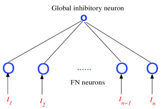
Figure 1: Diagram of the network. There are $n$ FN neurons receiving different external stimulating inputs. A global inhibition neuron monitors the network.

As illustrated in Figure 1, the network consists of $n$ FN neurons. Each neuron receives a stimulating input $I_{i}$ from outside as well as a common inhibition current $z$ from the global inhibition neuron. The dynamics of the FN neurons ($i=1,\ldots,n$) are

$$\begin{cases}\ \dot{v}_{i}=v_{i}(\alpha-v_{i})(v_{i}-1)-w_{i}+I_{i}-z\\ \ \dot{w}_{i}=\beta v_{i}-\gamma w_{i}\end{cases}$$

The dynamics of the global inhibition neuron switches between a charging mode and a discharging mode. It starts charging if there is any FN neuron spiking in the network, i.e. when $v_{i}$ exceeds a given threshold value $v_{0}$. It switches to discharging if the state is saturated (enough close to the saturation value in simulation) and stays at this mode until next time a FN neuron spikes. The specific dynamics of these two modes can be very general. For simplicity, we use

$$\dot{z}=\begin{cases}\ -k_{c}\ (z-z_{0})\ \ \ \ \mathrm{charging}\ \mathrm{mode}\\ \ -k_{d}\ z\ \ \ \ \ \ \ \ \ \ \ \ \mathrm{discharging}\ \mathrm{mode}\end{cases}$$

where $z_{0}$ is a constant saturation value, and $k_{c}$ and $k_{d}$ are the charging rate and discharging rate.

Within at most two periods, the winner will be the only neuron spiking in the whole network. In some cases, this is achieved within the first period.

To perform WTA computation, we set the charging rate of the global neuron to be fast and the discharging rate to be slow. Thus, similarly to [8], if there is any FN neuron spiking, the strength of the inhibition current increases to its saturation value very rapidly, leaving no chance for the other neurons to spike. The global neuron then discharges slowly, which lets the FN neurons smoothly approach the oscillation region. The first neuron entering the oscillation region will be the one with the largest input. So it spikes as the winner and ignites a new period. Note that before enter the oscillation region, all FN neurons converge to their equilibrium points with the equilibrium point of the winner having the largest value. A slowly discharging process allows the winner to occupy the highest position and helps it to spike immediately once it enters the oscillation region. Given the parameters of the FN neurons, the frequency of the result depends on the global neuron’s saturation value, its charging and discharging rates, and the value of the largest input. If we also fix the global neuron dynamics, the frequency increases with the increasing of the largest input. Simulation results are shown in Figure 2.

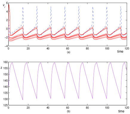
Figure 2: Simulation result of WTA computation with $n=10$. The parameters of the FN neurons are set as $\alpha=5.32,\beta=3,\gamma=0.1$, with spiking threshold $\ v_{0}=5\$. The inputs $I_{i}$ are chosen randomly from $20$ to $125$. The parameters of the global neuron are $z_{0}=160,k_{c}=1,k_{d}=1/50$. All the initial conditions are chosen arbitrarily. (a) States $v_{i}$ versus time. The dashed curve represents the state of the neuron receiving the largest input. (b) State $z$ versus time.

Remarks

$\bullet$ Initial conditions and computation speed     The mechanism described above guarantees that initial conditions can be set arbitrarily, which cannot be realized by most of the previous WTA models. With appropriate parameters, the computation can be completed at most in two periods. The first spiking neuron is chosen by initial conditions, while the second one is the neuron with the largest input, which remains the winner until the inputs change. Actually, if the initial inhibition is set large enough so that all the FN neurons are depressed in the beginning, then the neuron with the largest input will spike first. The computation speed of our FN network is faster and more robust than the WTA model recently presented in [8], whose network of integrate-and-fire neurons has to wait until the winner gets the right to spike, which may take a long time for large networks.

$\bullet$ Varying inputs and noise      Since initial conditions do not matter in our model, the network can easily track time-varying inputs. Figure 3 illustrates such an example, where three inputs switch winning positions several times. The spiking neuron always tracks the largest input. The computation is robust to signal noise as well.

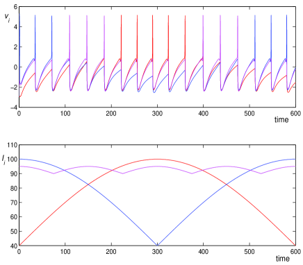
Figure 3: Simulation result of WTA computation with varying input. The parameters are all equal to those in Figure 2 except that $n=3$. Inputs change continuously. The winner always tracks the neuron with the largest input.

$\bullet$ Multiple winners     Decreasing the global neuron discharging rate $k_{d}$ extends the waiting time before the winner enters the oscillation region. This is helpful if there exist several neurons receiving the same largest input and we expect them all spike as a group of winners. Enlarging the time neurons stay in the stable region allows these neurons with the same input converge to each other, and to enter the oscillation region and spike simultaneously ( Figure 4). Note that in [8], only one winner can succeed and it is picked arbitrarily from the group of candidates.

If the network size is small, the network may be augmented with all-to-all couplings between FN neurons, with the coupling gain increasing with the similarity of the inputs (e.g., of the form $e^{-\ \alpha|\ I_{j}-I_{i}\ |}$ ). This lets the neurons receiving identical inputs converge together exponentially (using partial contraction theory [16]) and thus provides another solution to the multiple-winner problem.

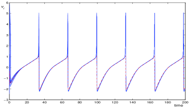
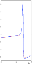
Figure 4: Simulation result of WTA computation with multiple winners. The parameters are the same as in Figure 2 except that $k_{c}=5,\ k_{d}=1/80$. The inputs are $\ I_{1}=\cdots=I_{9}=120,I_{10}=119.5\$. The first plot shows the $v_{i}$’s as functions of time. The dashed (red) line represents $v_{10}$ and the solid (blue) lines the other $v_{i}$’s. The first nine neurons converge together during the waiting time and spike simultaneously as a group of winners. The second plot, an enlarged version of the first at a spiking moment, shows that $v_{10}$ is completely depressed by the winners even though the input difference is very small.

$\bullet$ Computation resolution     Computation resolution can be improved by decreasing the global neuron discharging rate $k_{d}$ while increasing the charging rate $k_{c}$. Decreasing $k_{d}$ allows the winner fully distinguished with the following neurons; increasing $k_{c}$ prevents the following neurons spike after the winner. Figure 4 illustrates such an example with winners $I_{max}=120$ while the second largest input $I_{10}=119.5$. The resolution here is much better than the WTA models presented previously, including [11, 17]. It can be further enhanced by decreasing the relaxation time of the FN neurons.

$\bullet$ Input bounds     The inputs to the FN neurons should be lower-bounded by $I_{l}$ (the lower threshold of the oscillation region) to guarantee that the neurons can spike before the inhibition is fully released. They should also be upper bounded to set $z_{0}$.

$\bullet$ $K$-Winner-Take-All     $K$-Winner-Take-All ($k$-WTA) is a common variation of WTA computation [13], where the output indicates for each neuron whether its input is among the $k$ largest. An example $k$-WTA circuit in [17] extends the WTA model in [11] by formulating the problem in terms of mathematical programming, but it inherits its low resolution limit from [11] as well. Conversely, the advantages of the above FN network generalize to the $k$-WTA case. As inhibition decreases, the FN neurons enter the oscillation region rank-ordered by their inputs. For WTA computation, we charge the inhibition neuron after the first arrival. For $k$-WTA computation, we only need to modify the charging moment to capture the $k^{\rm th}$ arrival instead. Since the neurons enter the oscillation region in sequence, they spike in sequence. If we set $k=n$, we get a pre-ordered spiking sequence in each period, which may be used to realize soft-WTA [13, 19], and also provides a simple desynchronization mechanism for binding problems [6]. The computation resolution follows directly from that in WTA. A detailed description and discussion of the $k$-WTA network will be presented separately.

$\bullet$ Spike-controlled coupling and slow inhibition     The feedforward and recurrent connections used in our WTA network are similar to those in [9], where a “universal” control system is developed based on olivo-cerebellar networks. The couplings inside the circuit are also spike-controlled and they use a FitzHugh-Nagumo-like model containing four variables. A similar mechanism is also used in [18], where WTA is implemented to compute the object with the largest size. Slowly-discharged inhibition is also used in biologically motivated models such as [10, 18].

$\bullet$ Computational complexity      The complexity of the network is $O(n)$. Since the FN neurons are independent, they can be added or removed from the network at any time.

4 Fast Coincidence Detection

Recent neuroscience research suggests that coincidence detection plays a key role in temporal binding [12]. Hopfield et al. [2] proposed two neural network structures, both able to capture a “many-are-equal” moment, to model speech recognition and olfactory processing. A similar computation can be implemented by FN neurons, with faster and more salient response.

Consider a leader-followers network with a structure similar to Figure 1, except that the global neuron (the leader) is now excitatory, and the connections from the leader to the followers are unidirectional. For simplicity, we assume that all the neurons are FN neurons with the same parameters but different inputs. The dynamics of the leader $(v_{o},w_{o})$ obeys equations (1) while those of the followers ($i=1,\ldots,n$) are

$$\begin{cases}\ \dot{v}_{i}=v_{i}(\alpha-v_{i})(v_{i}-1)-w_{i}+I_{i}+k(v_{0}-v_{i})\\ \ \dot{w}_{i}=\beta v_{i}-\gamma w_{i}\end{cases}$$

where $k(v_{0}-v_{i})$ is the coupling force from the leader to the followers. Neurons $i$ and $j$ synchronize only if inputs $I_{i}$ and $I_{j}$ are identical. We define the system output accordingly to capture the moment when this condition becomes true for a large number of inputs, as illustrated in Figure 5. Note that the coupling gain $k$ should be large enough to guarantee synchronization (an explicit threshold can be computed analytically [16]), but not so large as to have the leader numerically dominate the dynamic differences between the followers. More general formal studies of synchronization can be found in [16], based on nonlinear contraction theory.

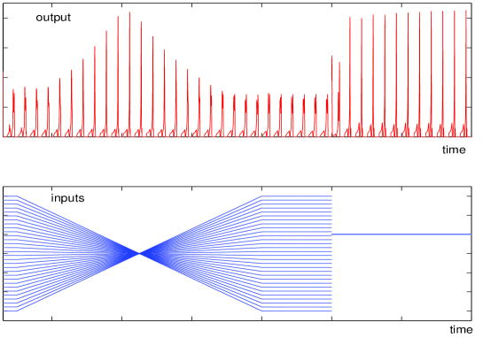
Figure 5: Simulation result of fast coincidence detection with $n=30$. The leader and the followers are FN neurons with the same parameters as in Figure 2. The inputs are $I_{0}=90$ and $I_{1},\ldots,I_{30}$ varying from $20$ to $80$, and the coupling gain is $k=1.7$. The upper plot shows $\ \sum_{i=1}^{n}\max(0,\dot{v_{i}})$ versus time, and the lower $I_{1},\ldots,I_{n}$.

5 Concluding Remarks

Basic computations such as winner-take-all and coincidence detection can be performed fast and robustly using extremely simple spike-based models. The results are currently being extended to higher-level perception problems.

Acknowledgments: This work was supported in part by a grant from the National Institutes of Health. The authors benefited from stimulating discussions with Matthew Tresch.

References

- [1] Arbib, M.A., MIT Press (1995); Amari, S., and Arbib, M., in Sys. Neurosci., 119 (1977); Ermentrout, B., Neural Networks, 5(3) (1992); Fang, Y., Cohen, M., and Kincaid, M., Neural Networks, 9:1141 (1996); Grossberg, S., Stud. in Appl. Math., 52:217 (1973); Grossberg, S., J. of Math. Analy. and Appl., 66:470 (1978); Indiveri, G., IEEE Internat. Joint Conf. on Neural Networks, 4:24 (2000)
- [2] Brody, C.D., and Hopfield, J.J., Neuron, 37:843 (2003); Hopfield, J.J., and Brody, C.D., Proc. Natl. Acad. Sci. USA, 98:1282 (2001)
- [3] Dehaene, S., et al., PNAS 95:14529 (1998); Gerstner, W., In The Handbook of Bi. Phy., 4:469 (2001); Izhikevich, E.M., IEEE Trans. on Neural Networks, (2003); Llinás, et al., Phil. Trans. R. Soc. Lond. 353:1841 (1998); Maass, W., Natschlger, T., and Markram, H. (2003); Thorpe, S., et al., Nature, 381:520 (1996); Thorpe, S., et al., Neural Networks, 14:715 (2001)
- [4] Feldman, J.A., and Ballard, D.H., Cognit. Sci., 6:205 (1982); Yuille, A.L., and Grzywacz, N.M., Neural Comput., 1:334 (1989)
- [5] FitzHugh, R.A., Biophys. J., 1:445 (1961); Nagumo, J., et al., Proc. Inst. Radio Engineers, 50:2061 (1962)
- [6] Gray, C.M., Neuron, 24:31 (1999); Singer, W., and Gray, C.M., Annu. Rev. Neurosci., 18:555 (1995); von der Malsburg, C., Current Opinion in Neurobio., 5:520 (1995); Wang, D.L., The Time Dimension for Neural Computation, (2002)
- [7] Hodgkin, A.L., and Huxley, A.F., J. Physiol., 117:500 (1952)
- [8] Jin, D.Z., and Seung, H.S., Phy. Rev. E, 65:051922 (2002)
- [9] Kazantsev, V.B., et al., PNAS, 100:13064 (2003)
- [10] LoFaro, T., et al., Neural Comput., 6:69 (1994); Wang, X.J., and Rinzel, J., Neural Comput., 4:84 (1992)
- [11] Lazzaro, J., et al., in Advan. in Neural Info. Proc. Sys. 1. 703 (1988)
- [12] Llinás, et al., PNAS, 99:449 (2002); Tononi, G., et al., PNAS 95:3198 (1998)
- [13] Maass, W., Neural Comput., 12:2519 (2000); Maass, W., in Advan. in Info. Proc. Sys., 12:293 (2000)
- [14] Murray, J.D., Mathematical Biology, (1993)
- [15] Slotine, J.J.E., and Li, W., Applied Nonlinear Control, (1991); Strogatz, S.H., Nonlinear Dynamics and Chaos, (1994)
- [16] Slotine, J.J.E., and Wang, W., in Cooper. Contr., Springer-Verlag, (2003); Wang, W., and Slotine, J.J.E., Biol. Cybern., submitted (2003)
- [17] Urahama, K., and Nagao, T., IEEE Trans. on Neural Networks,6:776 (1995)
- [18] Wang, D.L., Neural Networks, 12:579 (1999)
- [19] Yuille, A.L., and Geiger, D., in The Handbook of Brain Theory and Neural Networks, (2002)