Deriving the respiratory sinus arrhythmia from the heartbeat time series using Empirical Mode Decomposition

Abstract

Heart rate variability (HRV) is a well-known phenomenon whose characteristics are of great clinical relevance in pathophysiologic investigations. In particular, respiration is a powerful modulator of HRV contributing to the oscillations at highest frequency. Like almost all natural phenomena, HRV is the result of many nonlinearly interacting processes; therefore any linear analysis has the potential risk of underestimating, or even missing, a great amount of information content. Recently the technique of Empirical Mode Decomposition (EMD) has been proposed as a new tool for the analysis of nonlinear and nonstationary data. We applied EMD analysis to decompose the heartbeat intervals series, derived from one electrocardiographic (ECG) signal of 13 subjects, into their components in order to identify the modes associated with breathing. After each decomposition the mode showing the highest frequency and the corresponding respiratory signal were Hilbert transformed and the instantaneous phases extracted were then compared. The results obtained indicate a synchronization of order 1:1 between the two series proving the existence of phase and frequency coupling between the component associated with breathing and the respiratory signal itself in all subjects.

, , , , , ,

1 Introduction

Oscillations in heart rate on a beat by beat basis are a well-known phenomenon of great clinical relevance for both diagnostic and prognostic purposes. Many different factors (i.e. neural, chemical, hormonal modulations) contribute to the heart rate variability (HRV)  [1]. Among them, a major influence is exerted by the activity of the Sympathetic and Parasympathetic (vagal) branches of the Autonomic Nervous System (ANS)  [2]. In particular, respiration is a powerful modulator of HRV acting under the control of the ANS parasympathetic branch; in addition, abnormalities in respiratory modulation are often an indication of autonomic disfunction  [3, 4].

Traditionally HRV analysis is accomplished, in the frequency domain, via spectral analysis of the heartbeat time series (RR intervals) and, in the time domain, by extracting statistical indexes not related to specific cycle lengths. Parasympathetic activity is primarily reflected in the high-frequency (HF) component of the power spectrum (0.15-0.40 Hz) and it is related to the breathing frequency (respiratory sinus arrhythmia, RSA). More controversial is the interpretation of the low-frequency (LF) component (0.04-0.15 Hz), which is considered by some investigators as a marker of sympathetic modulation  [5, 6] and by others as influenced by both the sympathetic and parasympathetic activity  [7]. In the clinical environment a widely used index of sympathovagal balance is the ratio LF/HF.

For what concerns time domain indexes, they all measure high frequency variations in heart rate (and thus they are all highly correlated). An extensive introduction to HRV measurements can be found in  [2, 8].

Both time-domain and spectral methods share limitations imposed by the intrinsic nature of the RR series. In fact, changes in autonomic modulations can occur because of a variety of common factors such as changing position from sitting to standing, eating, running, sleeping, wakening. This can induce both a lack of stationarity in the series, compromising a correct application of these methods, and a shift of the LF and HF central frequencies, with a possible superposition of the two bands and a consequent misleading interpretation.

Other methods estimate RSA through a linear model by using an adaptive filter scheme having the respiratory signal as reference input  [9]. The first limitation of these approaches is the need of the respiratory signal. The second concerns the approximation of the linear model that is not always acceptable. Like almost all natural phenomena, HRV is the result of many nonlinearly interacting processes; therefore any linear analysis has the potential risk of underestimating, or even missing, a great amount of information content. On the other hand, complex nonlinear approaches  [10] do not provide the tracking capability required in the high non-stationary context of RR interval series.

Recently the Empirical Mode Decomposition (EMD), a signal processing technique particularly suitable for nonlinear and nonstationary series, has been proposed  [11] as a new tool for data analysis. This technique performs a time adaptive decomposition of a complex signal into elementary, almost orthogonal components that do not overlap in frequency. The extracted components have well behaved Hilbert transforms, from which the instantaneous frequencies can be calculated.

We applied EMD analysis to decompose the RR series into its components in order to identify, primarily, the respiratory oscillation. For comparison purpose, the respiratory signal was recorded simultaneously with the electrocardiogram (ECG). The existence of phase and frequency coupling between the RR component associated with breathing and the respiratory signal itself was then investigated.

2 Empirical Mode Decomposition

The empirical mode decomposition is a signal processing technique proposed in 1998 by Huang  [11] to extract all the oscillatory modes embedded in a signal without any requirement of stationarity or linearity of the data. The goal of this procedure is to decompose a time series into components with well defined instantaneous frequency by empirically identifying the physical time scales intrinsic to the data, that is the time lapse between successive extrema.

Each characteristic oscillatory mode extracted, named Intrinsic Mode Function (IMF), satisfies the following properties: an IMF is symmetric, has a unique local frequency, and different IMFs do not exhibit the same frequency at the same time. In other words the IMFs are characterized by having the number of extrema and the number of zero crossings equal (or differing at most by one), and the mean value between the upper and lower envelope equal to zero at any point.

The algorithm operates through six steps:

1. Identification of all the extrema (maxima and minima) of the series $X$.

2. Generation of the upper and lower envelope via cubic spline interpolation among all the maxima and minima, respectively.

3. Point by point averaging of the two envelopes to compute a local mean series $m$.

4. Subtraction of $m$ from the data to obtain a IMF candidate $h=X-m$.

5. Check the properties of $h$:

   • if $h$ is not a IMF (i.e. it does not satisfy the previously defined properties), replace $X$ with $h$ and repeat the procedure from step 1

   • if $h$ is a IMF, evaluate the residue $r=X-h$.

6. Repeat the procedure from step 1 to step 5 by sifting the residual signal. The sifting process ends when the residue $r$ satisfies a predefined stopping criterion.

At the end of the procedure we have a residue $r$ and a collection of $n$ IMFs, named $h_{i}$ ($i=1,...,n$). The $h_{i}$ are generated being sorted in descending order of frequency and therefore $h_{1}$ is the one associated with the locally highest frequency. Furthermore the original $X$ can be exactly reconstructed by a linear superposition:

$$X=\sum_{i=1}^{n}h_{i}+r.$$

Usually to eliminate riding waves and obtain symmetric waves, the sifting process has to be repeated a number of times. To verify whether $h$ owns the IMF properties (step 5 of the sifting procedure) we used a range-based criterion: $h$ is retained as IMF if the range of $m$ is a very low fraction of that of $h$ $(<0.001)$.

Analogously, for what concerns the stopping criterion of the EMD iterations, when all the interesting intrinsic modes of the original series have been extracted, we checked the range of $r$: the sifting process ends when the range of the residue is low with respect to that of the original signal ($<10\%$).

Figure  1 shows the starting point of a signal decomposition and the IMF candidate obtained after few iterations. Figure  2 shows an example of EMD decomposition of a simulated series obtained by linear composition of three different nonstationary oscillations.

The EMD procedure, according to the above specifications, was used for the decomposition of the RR interval series (tachograms) as described in the next section.

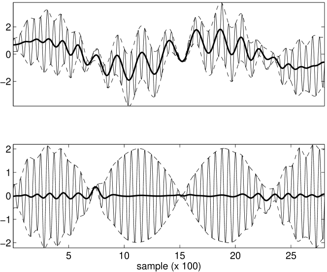
Figure 1: Upper panel: the original signal with upper and lower envelope. The thick line represents the point by point mean value of the envelopes. Lower panel: the signal $h$ after few iterations. The iterations continue until $h$ becomes a IMF.

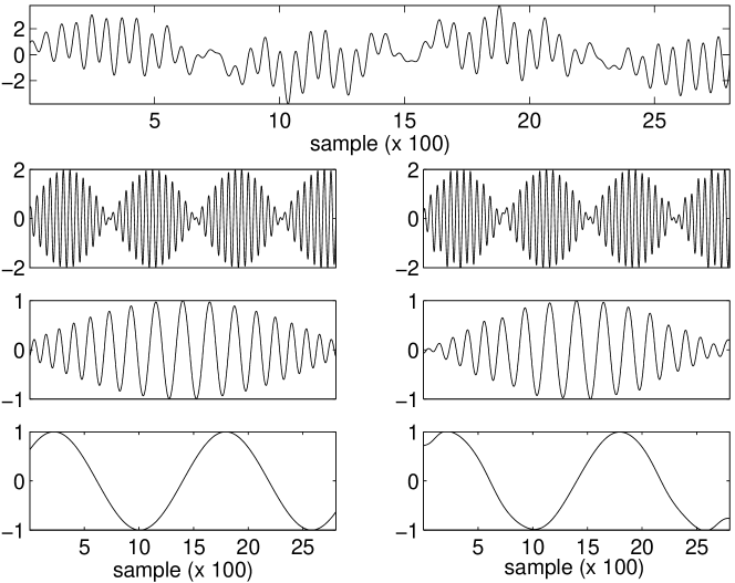
Figure 2: Upper panel: the artificial series of 2800 points obtained by linear combination of three oscillatory signals shown in the left column. Right column: the IMF extracted using EMD.

3 Experimental procedure

Thirteen healthy volunteers underwent an experimental session in which one electrocardiographic (ECG) derivation and the respiratory signal were simultaneously and continuously acquired at 1000 Hz sampling frequency. The ECG was recorded using standard electrodes, while the respiratory signal was detected through a polymeric piezoelectric dc-coupled transducer inserted into a belt wrapped around the chest. During the experimental session the subjects were comfortably sitting and breathing freely.

From the ECG signal, R waves, indicating the ventricular depolarization, were detected to obtain the tachogram, that is the series of the time intervals between the occurrence of two consecutive R peaks. The tachogram was then interpolated at 1 Hz, to obtain uniformly time spaced data.

The respiratory signals were bandpass filtered in the respiratory range 0.15-0.4 Hz  [2] to remove artifacts mainly due to the positioning of the chest belt and its mechanical properties. The respiratory signal was then decimated according to the corresponding interpolated tachogram, thus making the two series syncronous. The tachograms of the 13 subjects were decomposed using EMD and each first component was analyzed together with the corresponding respiratory signal.

4 Instantaneous frequency analysis

The local frequency of each IMF can be expressed by the instantaneous frequency defined by virtue of the analytic signal of the original data.

Given a real function $f(t)$ with Fourier transform $F(\nu)$, the analytic signal $f_{a}(t)$ is defined as the inverse Fourier transform of the positive frequency part of $F(\nu)$:

$$f_{a}(t)=2\,\int_{0}^{+\infty}F(\nu)e^{j\,2\pi\nu t}dv.$$

The real part of $f_{a}(t)$ is just $f(t)$ while the imaginary part defines the Hilbert transform of $f(t)$ ($f_{H}(t)$). Thus $f_{a}(t)=f(t)+jf_{H}(t)=a(t)\exp{j\phi(t)}$ in which:

$$a(t)=(f^{2}(t)+f_{H}^{2}(t))^{\frac{1}{2}}\quad\quad\phi(t)=\arctan\frac{f_{H}(t)}{f(t)}.$$

The instantaneous frequency is defined as the rate of phase change:

$$\nu(t)=\frac{d\phi(t)}{dt}.$$

We investigated the phase relationship between the first IMF and the respiratory signal by computing the instantaneous phases $\phi_{1}$ and $\phi_{2}$ from both signals and looking at their behavior by plotting $\phi_{1}$ mod $2\pi$ versus $\phi_{2}$, mod $2\pi$ (bi-plot).

When a phase locking exists, the points in the bi-plot are not uniformly distributed and some structure is visible  [12, 13, 14, 15]. In case of linear phase coupling, the points in the bi-plot are ideally aligned along a straight line, in practice they cluster along a stripe whose slope indicates the frequency ratio (synchronization order) of the two signals.

The stripe slope was estimated through a generalized regression, that is detecting the direction of the eigenvector associated to the highest eigenvalue (maximum variance direction) via a Principal Components Analysis (PCA) procedure  [16]. The goodness of the relationship was measured by the residual variance, an index of the spread of points along the orthogonal direction. The instantaneous frequencies were computed using the toolbox Time-frequency toolbox for Matlab (TFTB)  [17].

5 Results

The tachograms of all the 13 subjects were decomposed using EMD. The number of the oscillatory modes extracted ranged between 5 and 8 (median 7).

Since the breathing frequency is the highest frequency contributing to HRV, the first IMF (IMF1) generated was used for comparison with the recorded respiratory signal. For each subject IMF1 and the recorded respiratory signal were Hilbert-transformed and the instantaneous phases computed. Figure  3 shows the tachogram and and the simultaneous respiratory signal of one subject.

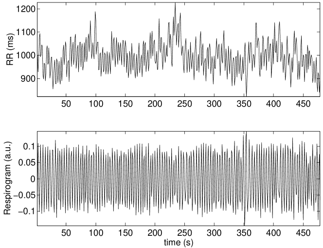
Figure 3: An example of tachogram (upper) with simultaneous respiratory time series (lower).

The relative phase distribution $\Delta\phi$ = $\phi_{1}-\phi_{2}$ shown in figure  4 exhibits a sharp peak suggestive of a coupling between $\phi_{1}$ and $\phi_{2}$. An example of the close correspondence between the two series of instantaneous frequencies is presented in figure  5.

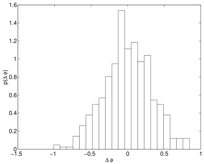
Figure 4: Distribution of phase differences between recorded respirogram and IMF1.

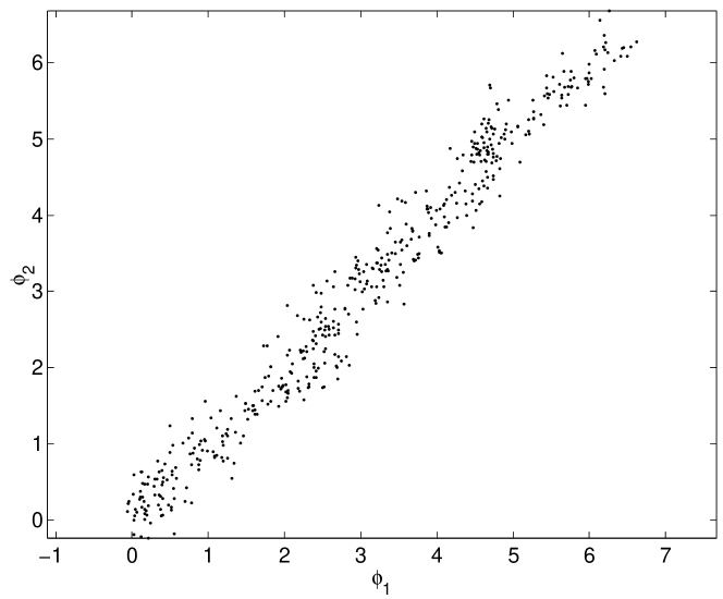
Figure 5: Relationship between respirogram anda IMF1 phases.

The average frequency ratio between each couple of signals is $1.015\pm 0.017$ which is very close to 1, as expected for a synchronization of order 1:1. The average residual variance is 3.7%, indicating a good linear relationship.

6 Discussion

The Empirical Mode Decomposition technique allows the analysis of complex, nonlinear and nonstationary time series, through their decomposition into a limited number of elementary modes having interesting local properties. In the EMD applications reported in literature  [18, 19, 20, 21], the extracted modes are speculatively associated with specific physical or physiological aspects of the phenomenon investigated. In this application we demonstrated the association of the first IMF extracted from a tachogram with the simultaneously recorded respiratory signal.

The EMD implementation required some computational skills essentially to cope with the selection of the stopping criteria for both sifting and EMD processes and the management of the end points for cubic splines interpolation. The selected criteria were not necessarily unique: in any case the procedure is robust with respect to a variety of different solutions.

The peculiar property of each IMF of having a single local frequency was particularly suitable to compute the instantaneous phases and frequencies after Hilbert transformation. According to  [12], in order to verify the synchronization between the two series, we focused on the phases relationship. We preferred to work with instantaneous phases instead of frequencies for that the former resulted to be more stable in time. The series of frequencies shown in figure  6 are indeed not instantaneously derived, but computed with a smoothing factor from the toolbox TFTB.

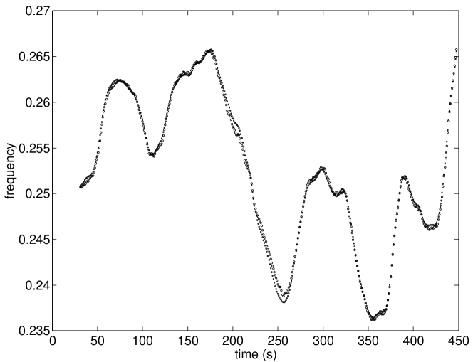
Figure 6: Instantaneus frequencies obtained by Hilbert transform of respirogram and IMF1.

The linear relationship and the generalized regression slope closest to 1 confirmed the synchronization between $\phi_{1}$ and $\phi_{2}$ and therefore the substantial correspondence between the IMF1 and respiratory time series. The importance of this finding is essentially two-fold for the physiologist. First, the instantaneous respiratory contribution can now be available even in all those retrospective studies where the breathing signal was lacking. Second, the possibility of selectively and efficiently eliminate the respiratory component from the tachogram makes possible a more accurate evaluation of the LF role in ANS studies.

Our goal is now to proceed with this approach in the attempt of attributing a physiological meaning to the other modes embedded in the tachogram in order to improve the knowledge of the pathophysiological mechanisms underlying heart rate variability.

References

- [1] Malliani A. Principles of Cardiovascular Neural Regulation in Health and Disease. Kluwer Academic Publishers, 2000.
- [2] Task Force of The European Society of Cardiology, The North American Society of Pacing, and Electrophysiology. Heart rate variability. European Heart Journal, (17):354–381, 1996.
- [3] Bernardi L, Porta C, Gabutti A, Spicuzza L, and Sleight P. Modulatory effects of respiration. Autonomic Neuroscience: Basic and Clinical, (90):47–56, 2001.
- [4] Pinna GD, Maestri R, Mortara A, and La Rovere MT. Cardiorespiratory interactions during periodic breathing in awake chronic heart failure patients. Am. J. Physiol. Heart Circ. Physiol., 278:H932–H941, 2000.
- [5] Sleight P and Bernardi P. Sympathovagal balance. Circulation, 98:2640, 1998.
- [6] Malliani A, Pagani M, Montano N, and Mela S. Sympathovagal balance: A reappraisal. Circulation, 98:2640–2642, 1998.
- [7] Eckberg DL. Sympathovagal balance: a critical appraisal. Circulation, 96:3224–3232, 1997.
- [8] Committee to Revise the Guidelines for Ambulatory Electrocardiography. Acc/aha guidelines for ambulatory electrocardiography. Journal of the American College of Cardiology, (3):913–948, 1999.
- [9] Varanini M, Emdin M, and Raciti M. Adaptive filtering for cancelling/enhancing the respiratory contribution to cardiovascular signals. J Ambul Monit, (5):95–105, 1992.
- [10] Varanini M, Macerata A, Emdin M, and Marchesi C. Non linear filtering for the estimation of the respiratory component in heart rate. In Computers in Cardiology, pages 565–568. IEEE Computer Society, 1994.
- [11] Huang NE, Shen Z, Long SR, Wu MC, Shih HH, Zheng Q, Yen N, Tung CC, and Liu HH. The empirical mode decomposition and the hilbert spectrum for nonlinear and non-stationary time series analysis. Proc. R. Soc., A(454):903–995, 1998.
- [12] Palus M and Hoyer D. Detecting nonlinearity and phase synchronization with surrogate data. IEEE Eng Med Bio Mag, (17):40–45, 1998.
- [13] Rosenblum MG, Kurths J, Pikovsky A, Schafer C, Tass P, and Abel H. Synchronization in noisy systems and cardiorespiratory interaction. IEEE Eng Med Bio Mag, (17):46–53, 1998.
- [14] Toledo E, Rosenblum MG, Schafer C, Kurths J, and Akselrod S. Quantification of cardiorespiratory synchronization in normal and heart transplant subjects. In International Symposium on Nonlinear Theory and its Applications, pages 171–174. T. Kohda and M.J. Ogorzalek, Presses Polytechniques et Universitaires Romandes Crans-Montana, 1998.
- [15] Schafer C, Rosenblum MG, and Kurths J. Heartbeat synchronized with ventilation. Nature, (392):239–240, 1998.
- [16] Mardia KV, Kent JT, and Bibby JM. Multivariate Analysis. Academic Press, London, 1994.
- [17] Auger F, Flandrin P, Goncalves P, and Lemoine O. Time-frequency toolbox for matlab. http://crttsn.univ-nantes.fr/ auger/tftb.html.
- [18] Huang NE, Shen Z, and Long SR. A new view of nonlinear water waves: the hilbert spectrum. Annu. Rev. Fluid Mech, (31):417–457, 1999.
- [19] Liang H, Lin Z, and McCallum RW. Artifact reduction in electrogastrogram based on empirical mode decomposition method. Med Biol Eng Comput, (38):35–41, 2000.
- [20] Neto EPS, Custaud MA, Cejka JC, Abry P, Frutoso J, Gharib C, and Flandrin P. Assessment of cardiovascular autonomic control by the empirical mode decomposition. In 4th International Workshop on Biosignal interpreatation, pages 123–126. Polytechnic University, Milano, Italy, 2002.
- [21] Huang W, Shen Z, Huang NE, and Fung YC. Engineering analysis of biological variables: an example of blood pressure over 1 day. Proc. Natl. Acad. Sci. USA, (95):4816–4821, 1998.