Multi-Stability in Monotone Input/Output Systems

Abstract This paper studies the emergence of multi-stability and hysteresis in those systems that arise, under positive feedback, starting from monotone systems with well-defined steady-state responses. Such feedback configurations appear routinely in several fields of application, and especially in biology. Characterizations of global stability behavior are stated in terms of easily checkable graphical conditions.

Keywords: monotone systems, bistability, hysteresis, multiple steady-states

1 Introduction

Multi-stability and associated hysteresis effects form the basis of many models in molecular biology, in areas such as cell differentiation, development, and periodic behavior described by relaxation oscillations. See for instance the classic work by Delbrück [5], who suggested in 1948 that multi-stability could explain cell differentiation, as well as references in the current literature (e.g., [4], [11], [12], [13], [15], [19], [23], [31]).

One appealing class of systems in which to study this phenomenon is that of monotone systems with inputs and outputs, a class of systems introduced recently in [2], motivated by applications in molecular biology modeling. Monotone systems with inputs and outputs constitute a natural generalization of classical (no inputs and outputs) monotone dynamical systems, which are those for which flows preserve a suitable partial ordering on states. The work reported here is grounded upon the rich and elegant theory of monotone dynamical systems (see the textbook by Smith [27] as well as papers such as [17, 16] by Hirsch and [25] by Smale), which provides results on generic convergence to equilibria, and, more generally, on the precise characterization of omega limit sets. One of the main difficulties in applying the theory of monotone dynamical systems is that of determining the locations and number of steady states. In this paper, we propose the idea of viewing more complicated systems as positive feedback loops involving monotone systems with inputs and outputs and well-defined steady state responses. The feedback configuration may induce multiple steady states, and we show how the locations and stability of them can be completely characterized using a simple planar graphical test.

We present the general theory, and illustrate the results by means of two examples. The first is a simple two-dimensional system; since such systems can be analyzed using classical phase-plane techniques, the example can be related to routine and elementary calculations, and thus the meaning of our conditions is easy to understand. The second example is of high order, and arises in the study of cellular signaling cascades. Further applications are developed in the reference [1].

The organization of this paper is as follows. First, we review the basic definitions regarding monotone systems and state our main results regarding positive feedbacks. Then we present and prove several graphical tests which are useful in checking the properties required by our results. After this, we provide proofs of the main theorems as well as a number of needed technical facts concerning linear systems which arise when linearizing general monotone systems along trajectories. This is followed by two examples, as discussed above. The paper closes with a discussion of hysteresis behavior, as well as a subtle counterexample showing that monotonicity plays a crucial role and cannot be dispensed with as an assumption. Two appendixes contain proofs of some technical points.

2 Basic Definitions

We briefly review some of the main concepts and notations from [2].

By a positivity cone $K$ in a Euclidean space ${\mathbb{B}}$ we mean a nonempty closed convex and pointed ($K\bigcap-K=\{0\}$) cone $K\subset{\mathbb{B}}$. In this paper, we assume that cones have nonempty interiors. Associated to such a cone, one introduces a partial ordering: $x_{1}\succeq x_{2}$ (or “$x_{2}\preceq x_{1}$”) iff $x_{1}-x_{2}\in K$. Strict ordering is denoted by $x_{1}\succ x_{2}$, meaning that $x_{1}\succeq x_{2}$ and $x_{1}\neq x_{2}$. One also introduces a stricter ordering by the rule: $x_{1}\gg x_{2}\Leftrightarrow x_{1}-x_{2}\in\textrm{int}(K)$. A typical example is ${\mathbb{B}}={\mathbb{R}}^{n}$ with the “NorthEast” ordering given by the first orthant: $K={\mathbb{R}}_{\geq 0}^{n}$, in which case “$x_{1}\succeq x_{2}$” means that each coordinate of $x_{1}$ is bigger or equal than the corresponding coordinate of $x_{2}$. In this case, $x_{1}\gg x_{2}$ means that every coordinate of $x_{1}$ is strictly larger than the corresponding coordinate of $x_{2}$, in contrast to “$x_{1}\succ x_{2}$” which means only that some coordinate is strictly larger.

State-spaces for monotone systems are by definition subsets $X$ of ${\mathbb{R}}^{n}$, for a suitable $n$, and endowed with an order arising from a cone $K^{X}$ (or just “$K$” if clear from the context). We assume always that $X$ is the closure of an open subset of ${\mathbb{R}}^{n}$. Input sets ${\mathcal{U}}$ are subsets of ordered spaces ${\mathbb{R}}^{m}$, and we write $u_{1}\succeq u_{2}$ whenever $u_{1}-u_{2}\in K^{\mathcal{U}}$ where $K^{\mathcal{U}}$ is the corresponding positivity cone in ${\mathbb{R}}^{m}$, for any pair of input values $u_{1}$ and $u_{2}\in{\mathcal{U}}$. An “input” is a locally essentially bounded Lebesgue measurable function $u(\cdot):{\mathbb{R}}_{\geq 0}\rightarrow{\mathcal{U}}$, and we write $u_{1}\succeq u_{2}$ provided that $u_{1}(t)\succeq u_{2}(t)$ for almost all $t\geq 0$. Similarly, output sets ${\mathcal{Y}}$ will be assumed to be ordered as well. To keep the notation simple and only when there is no risk of ambiguity, we use the same symbol for all orders.

A (finite-dimensional continuous-time) system in the sense of control theory (see e.g. [30])

$$\dot{x}\,=\,f(x,u)\,,\quad y=h(x)$$ (1)

is specified by a state space $X$, an input set ${\mathcal{U}}$, and an output set ${\mathcal{Y}}$, where the map $f$ is defined on $\widetilde{X}\times{\mathcal{U}}$, where $\widetilde{X}$ is some open subset of ${\mathbb{R}}^{n}$ which contains $X$. In general, one may assume that $f(x,u)$ is continuous in $(x,u)$ and locally Lipschitz continuous in $x$ locally uniformly on $u$, but for simplicity in this paper, we will assume that $f(x,u)$ is differentiable. In order to obtain a well-defined controlled dynamical system on $X$, we will assume that the solution $x(t)=\phi(t,\xi,u)$ (or just “$x(t,\xi,u)$”) of $\dot{x}(t)=f(x(t),u(t))$ with initial condition $x(0)=\xi$ is defined for all inputs $u(\cdot)$ and all times $t\geq 0$. This means that solutions with initial states in $X$ must be defined for all $t\geq 0$ (forward completeness) and that the set $X$ is forward invariant. We say that the system is monotone if the following property holds, with respect to the orders on states and inputs:

$$\xi_{1}\succeq\xi_{2}\quad\&\quad u_{1}\succeq u_{2}\quad\Rightarrow\quad x(t,\xi_{1},u_{1})\succeq x(t,\xi_{2},u_{2})\quad\forall\,t\geq 0.$$

If $\textrm{int}(K)\neq\emptyset$, this is equivalent to asking:

$$\xi_{1}\gg\xi_{2}\quad\&\quad u_{1}\succeq u_{2}\quad\Rightarrow\quad x(t,\xi_{1},u_{1})\gg x(t,\xi_{2},u_{2})\quad\forall\,t\geq 0$$

(a set which is the closure of its interior is invariant iff its interior is invariant, see [2]). We also assume given a monotone ($x_{1}\succeq x_{2}$ $\Rightarrow$ $h(x_{1})\succeq h(x_{2})$) output map $h:X\rightarrow{\mathcal{Y}}$, where ${\mathcal{Y}}$, the set of measurement or output values, is a subset of some ordered space ${\mathbb{R}}^{p}$.

We also recall the following definition: a system is strongly monotone if:

$$\xi_{1}\succ\xi_{2}\quad\&\quad u_{1}\succeq u_{2}\quad\Rightarrow\quad x(t,\xi_{1},u_{1})\gg x(t,\xi_{2},u_{2})\quad\forall\,t>0.$$

It is often convenient to assume more about the steady-state convergence properties of a monotone system. The following notion, first introduced in [2] in slightly weaker form, will be useful in order to state our main result.

Definition 2.1

We say that a system admits a non-degenerate input to state (I/S) static characteristic $k^{X}(\cdot):\mathcal{U}\rightarrow X$ if, for each constant input $u\in\mathcal{U}$, there exists a unique globally asymptotically stable equilibrium $k^{X}(u)$ and $\textrm{det}(D_{x}f(k^{X}(u),u))\neq 0$. $\Box$

Notice that, for technical reasons, the property has been strengthened with respect to the definition in [2] by assuming non-degeneracy of the equilibria. For systems with non-degenerate I/S characteristic, we also define their input/output (I/O) characteristic as the composition $h\circ k^{X}$.

Detecting if a system is monotone with respect to the partial order induced by some positivity cone $K$, without actually having to compute explicit trajectories of the system itself, is of course a very important task in order to apply our results in any specific situation. Necessary and sufficient differential characterizations of monotonicity are discussed in [2], where extensions to systems with inputs and outputs are presented of some well-known criteria previously only formulated for autonomous differential equations (see [27]). For the sake of completeness we recall the differential characterization proved in [2]. This characterization uses the concept of contingent cones to subsets of Euclidean spaces.

Theorem 1

A finite-dimensional nonlinear systems of differential equations $\dot{x}=f(x,u)$ with state-space $X$ and input-space $\mathcal{U}$ is monotone, with respect to positivity cones $K$ on states and $K^{\mathcal{U}}$ on inputs, if and only if:

$$x_{1}\succeq x_{2}\textrm{ and }u_{1}\succeq u_{2}\;\Rightarrow\;f(x_{1},u_{1})-f(x_{2},u_{2})\in{\cal T}_{x_{1}-x_{2}}K$$ (2)

where ${\cal T}_{x}K$ denotes the tangent cone to $K$ at the point $x$.  

An alternative characterization, also provided in [2], uses a generalization (to systems with inputs) of the concept of quasi-monotonicity: the system (1) is monotone if and only if

$$\begin{array}[]{rcl}\xi_{1}\succeq\xi_{2},\,u_{1}\succeq u_{2},\,\zeta\in K^{*},\mbox{ and }\langle\zeta,\xi_{1}\rangle=\langle\zeta,\xi_{2}\rangle\\ \Rightarrow\langle\zeta,f(\xi_{1},u_{1})\rangle\;\geq\;\langle\zeta,f(\xi_{2},u_{2})\rangle\end{array}$$

(it suffices to check this property for $\xi_{1}-\xi_{2}\in\partial K$), where $K^{*}$ is the set of all $\zeta\in{\mathbb{R}}^{n}$ so that $\langle\zeta,k\rangle\geq 0$ for all $k\in K$.

Orthant orders

Any orthant $K$ in ${\mathbb{R}}^{n}$ has the form

$$K^{(\varepsilon)}\;=\;\{x\in{\mathbb{R}}^{n}\;|\;(-1)^{\varepsilon_{i}}x_{i}\geq 0\,,\;i=1,\ldots,n\}$$

for some binary vector $\varepsilon=(\varepsilon_{1},\ldots,\varepsilon_{n})\in\{0,1\}^{n}$. Under appropriate changes of variables, one may often reduce the study of monotone systems to the special case in which states, inputs, and outputs are ordered with $K=$ the main orthant (all $\varepsilon_{i}=0$), i.e. to the study of cooperative systems. See [2] for details.

3 Statement of Main Results

The property defined next was studied for linear systems in [10].

Definition 3.1

A system is excitable if for any initial condition $\xi$ and any pair of inputs $v,u$ with $v\succ u$ for almost all $t>0$, the following holds:

$$x(t,\xi,v)\gg x(t,\xi,u)\qquad\forall\,t>0.$$ (3)

It is weakly excitable if this is required for any pair of inputs $v,u$ with $v\gg u$. $\Box$

The dual of excitability is also useful in the following discussion:

Definition 3.2

A system is transparent if for each input $u$, and each pair of solutions $x(t,\xi_{1},u)$, $x(t,\xi_{2},u)$ with $\xi_{1}\succ\xi_{2}$ we have $h(x(t,\xi_{1},u))\gg h(x(t,\xi_{2},u))$ for all $t>0$. It is weakly transparent if the conclusion is that $h(x(t,\xi_{1},u))\succ h(x(t,\xi_{2},u))$ for all $t>0$. $\Box$

We prove in Section 5 this sufficient condition for strong monotonicity of systems in unitary feedback:

Theorem 2

Consider the unitary feedback interconnection of a system (1), i.e. the system

$$\dot{x}=f(x,h(x))$$ (4)

resulting when we let $u=y$ and assume that inputs and outputs are ordered with respect to the same positivity cone. The induced flow is strongly monotone provided that (1) be monotone, excitable and transparent with either excitability or transparency possibly holding in a weak sense.

Our main result will provide a global analysis tool for systems obtained by positive feedback loops involving monotone systems. In [31], R. Thomas conjectured that the existence of at least one positive loop in the incidence graph is a necessary condition for the existence of multiple steady states. Proofs of this conjecture were given in [14], [22], [29], and [8], under different assumptions on the system (the last reference provides the most general result, using a degree theory argument). However, the existence of positive loops is not sufficient, and our main theorem deals precisely with this question.

The fixed points of the I/O characteristic will play a central role in the statement of the result. In particular, we say that a map $k:\mathcal{U}\rightarrow\mathcal{U}$ has non-degenerate fixed points if for all $u\in\mathcal{U}$ with $k(u)=u$ we have that $k^{\prime}(u)$ exists and $k^{\prime}(u)\neq 1$.

Theorem 3

Consider a monotone, single-input, single-output ($m=p=1$, with standard order) system, endowed with a non-degenerate I/S and I/O static characteristic:

$$\begin{array}[]{rcl}\dot{x}&=&f(x,u)\\ y&=&h(x).\end{array}$$ (5)

Consider the unitary positive feedback interconnection $u=y$. Then the equilibria are in 1-1 correspondence with the fixed points of the I/O characteristic. Moreover, if $k^{\mathcal{Y}}$ has non-degenerate fixed points, the closed-loop system is strongly monotone, and all trajectories are bounded, then for almost all initial conditions, solutions converge to the set of equilibria of (5) corresponding to inputs for which ${k^{\mathcal{Y}}}^{\prime}(u)<1$.

This theorem is proved in Section 7. The fact that equilibria correspond to fixed points of the characteristic is straightforward, but the global, and even local, stability statements are nontrivial. The result is particularly useful when combined with the characterization of strong monotonicity given in Theorem 2.

The next Section presents several graphical tests that are very useful in checking the properties required by our Theorems.

4 Graphical Conditions for Strong Monotonicity

For the special case of positivity orthants, i.e. when the orders in each of the input, state, and output spaces is defined by an orthant, criteria may be formulated in terms of the incidence graph of the system.

Along similar lines to [18], we associate to a given system (1) a signed digraph, with vertices $x_{1},x_{2}\ldots x_{n}$, $u_{1},u_{2},\ldots u_{m}$, $y_{1},y_{2}\ldots y_{p}$ and edges constructed according to the following set of rules:

Edges between $x$ vertices:

The graph is defined only for systems so that for any couple $1\leq i,j\leq n$ of integers with $i\neq j$ one of the following rules apply:

1. If $f^{i}(x,u)$ is strictly increasing with respect to $x_{j}$ for all $x,u\in X\times\mathcal{U}$ then we draw a positive edge $e_{ij}^{x}$ directed from vertex $x_{j}$ to $x_{i}$.

2. If $f^{i}(x,u)$ is strictly decreasing as a function of $x_{j}$ for all $x,u\in X\times\mathcal{U}$ then we draw a negative edge $e_{ij}^{x}$ directed from vertex $x_{j}$ to $x_{i}$.

3. Otherwise, $\frac{\partial f^{i}}{\partial x_{j}}=0$ for all $x,u$ and no edge from $x_{j}$ to $x_{i}$ is drawn.

Edges between $u$ and $x$ vertices:

The graph is defined only for systems so that for any couple of integers $i$, $j$ with $1\leq i\leq n$ and $1\leq j\leq m$ one of the following rules apply:

1. If $f^{i}(x,u)$ is strictly increasing as a function of $u_{j}$ for all $x,u\in X\times\mathcal{U}$ then we draw a positive edge ${e}_{ij}^{u}$ directed from vertex $u_{j}$ to $x_{i}$.

2. If $f^{i}(x,u)$ is strictly decreasing as a function of $u_{j}$ for all $x,u\in X\times\mathcal{U}$ then we draw a negative edge ${e}_{ij}^{u}$ directed from vertex $u_{j}$ to $x_{i}$.

3. Otherwise $\frac{\partial f^{i}}{\partial u_{j}}=0$ for all $x,u$ and no edge from $u_{j}$ to $x_{i}$ is drawn.

Edges between $x$ and $y$ vertices:

The graph is defined only for systems so that for any couple of integers $i$, $j$ with $1\leq i\leq p$ and $1\leq j\leq n$ one of the following rules apply:

1. If $h^{i}(x)$ is strictly increasing as a function of $x_{j}$ for all $x\in X$ then we draw a positive edge ${e}_{ij}^{y}$ directed from vertex $x_{j}$ to $y_{i}$.

2. If $h^{i}(x)$ is strictly decreasing as a function of $x_{j}$ for all $x\in X$ then we draw a negative edge $e_{ij}^{y}$ directed from vertex $x_{j}$ to $y_{i}$.

3. Otherwise, $\frac{\partial h^{i}}{\partial x_{j}}=0$ for all $x\in X$ and no edge from $x_{j}$ to $y_{i}$ is drawn.

When there is no risk of confusion, we just write from now on just “$e_{ij}$” to refer to an edge of the type $e_{ij}^{x}$, $e_{ij}^{u}$, or $e_{ij}^{y}$.

Under this convention, a directed path $\mathcal{P}$ is a finite sequence of vertices, $v_{n_{0}},v_{n_{1}}\ldots v_{n_{L}}$, such that each vertex appears at most once in the sequence and $e_{ij}$ is an edge whenever $v_{j},v_{i}$ appear consecutively in the path. The integer $L$, is called the length of the path and it is denoted by $L(\mathcal{P})$. By $\mathcal{P}_{i}$, we denote the $v_{n_{i}}$, the $i+1$-th, vertex of the path $\mathcal{P}$. A cycle, not necessarily directed, is a finite sequence of vertices $v_{n_{0}},v_{n_{1}}\ldots v_{n_{L}}$ such that $v_{n_{0}}=v_{n_{L}}$ and the constraint that either $e_{ij}$ or $e_{ji}$ is an edge whenever $v_{i}$ and $v_{j}$ appear consecutively in the cycle. The sign of a cycle is defined as the product of the signs of the edges comprising it, and the sign of a path is defined to be the product of the signs of its edges.

One of the main results in [18] is that an autonomous system (no inputs) is monotone with respect to some orthant if and only if its associated graph does not contain any negative cycles. An analogous result (basically with the same proof, which therefore we omit), holds for controlled systems:

Proposition 4.1

A system (1) which admits an incidence graph according to the above set of rules is monotone with respect to some orthants $K$, $K^{\mathcal{U}}$ and $K^{\mathcal{Y}}$ if and only if its graph does not contain any negative cycles. $\Box$

Remark 4.2

We remark that in this set-up we deliberately restricted the class of systems for which the incidence graph is defined. In [18] in fact the milder requirement that $\frac{\partial f^{i}}{\partial x_{j}}\geq 0$ for all $x$ together with $\frac{\partial f^{i}}{\partial x_{j}}>0$ for some $x$ is asked for in order to draw an edge between vertices $x_{i}$, $x_{j}$. This more general notion of incidence graph is however much more cumbersome to deal with if we want to give conditions for strong monotonicity of a system. $\Box$

This definition of incidence graph also provides the right set-up for easy geometrical characterizations of excitability and transparency; see [21] for systems with no inputs and outputs:

Theorem 4

A monotone system which admits an incidence graph is excitable provided that each $x_{i}$ is reachable through a directed path from any $u_{j}$, and it is weakly excitable provided that each $x_{i}$ is reachable through a directed path from some $u_{j}$,

It is worth pointing out that for the special case of positive linear systems the above results are proven in [10].

Theorem 4 is proved in an Appendix.

Similarly, we have:

Theorem 5

A monotone system which admits an incidence graph is (weakly) transparent provided that directed paths exist from any $x_{j}$ to any (at least one) output vertex $y_{i}$ .

The proof of Theorem 5 is analogous to that of Theorem 4, and is sketched in an Appendix.

5 Proof of Theorem 2

By Theorem 1, we know that

$$x_{1}\succeq x_{2}\;\&\;u_{1}\succeq u_{2}\;\Rightarrow f(x_{1},u_{1})-f(x_{2},u_{2})\in{\cal T}_{x_{1}-x_{2}}K\,$$ (6)

where $K$ is the positivity cone relative to the order $\succeq$. Let us first show monotonicity of the feedback loop system. Recall that $h$ is a monotone map, i.e.:

$$x_{1}\succeq x_{2}\;\Rightarrow\;h(x_{1})\succeq h(x_{2})$$ (7)

Therefore, if we combine (6) with (7) and we let $u_{1}=h(x_{1})$ and $u_{2}=h(x_{2})$ we obtain

$$x_{1}\succeq x_{2}\;\Rightarrow f(x_{1},h(x_{1}))-f(x_{2},h(x_{2}))\in{\cal T}_{x_{1}-x_{2}}K$$ (8)

which, by Theorem 1 in [2] is equivalent to monotonicity of the closed-loop system:

$$\dot{z}=f(z,h(z)).$$ (9)

In particular then, if we denote by $z(t,\xi)$ the solutions of (9) we have as a consequence of monotonicity:

$$\xi_{1}\succeq\xi_{2}\;\Rightarrow h(z(t,\xi_{1}))\succeq h(z(t,\xi_{2}))\qquad\forall\;t\geq 0.$$ (10)

Exploiting the fact that $z(t,\xi)=x(t,\xi,h(z(\cdot,\xi)))$ and (weak) strong transparency of (1) we obtain:

$$\xi_{1}\succ\xi_{2}\; \Rightarrow h(z(t,\xi_{1}))=h(x(t,\xi_{1},h(z(\cdot,\xi_{1}))))\gg(\succ)\;h(x(t,\xi_{2},h(z(\cdot,\xi_{1}))))$$ (11)

$$\succeq h(x(t,\xi_{2},h(z(\cdot,\xi_{2}))))=h(z(t,\xi_{2}))\qquad\forall\,t>0.$$

Finally, by (11) and weak (strong) excitability:

$$\xi_{1}\succ\xi_{2} \Rightarrow h(z(t,\xi_{1}))\gg(\succ)\;h(z(t,\xi_{2}))$$ (12)

$$\Rightarrow z(t,\xi_{1})=x(t,\xi_{1},h(z(\cdot,\xi_{1})))\gg x(t,\xi_{2},h(z(\cdot,\xi_{2})))=z(t,\xi_{2})\qquad\forall\;t>0$$

as desired.  

6 Monotone Linear Systems

We recall next some basic facts about linear monotone systems which will be of interest in the discussion of the main result.

Theorem 6

Let us consider the following finite dimensional linear system:

$$\dot{x}=Ax+Bu,\qquad y=Cx.$$ (13)

with $x\in{\mathbb{R}}^{n}$, $u\in{\mathbb{R}}^{m}$, $y\in{\mathbb{R}}^{p}$ and assume the state, input and output space equipped with some partial orders induced by the positivity cones $K^{X}$, $K^{\mathcal{U}}$ and $K^{\mathcal{Y}}$ respectively.

System (13) is a monotone control system with respect to the partial orders specified above if and only if:

1. $K^{X}$ is positively invariant for the autonomous system $\dot{x}=Ax$;

2. $BK^{\mathcal{U}}\subseteq K^{X}$;

3. $CK^{X}\subseteq K^{\mathcal{Y}}$.

Proof. By the characterization of monotonicity in Theorem 1, a system is monotone if and only if:

$$x_{1}\succeq x_{2}\;\&\;u_{1}\succeq u_{2}\quad\Rightarrow\quad A(x_{1}-x_{2})+B(u_{1}-u_{2})\in{\cal T}_{x_{1}-x_{2}}K^{X},$$ (14)

and the output map is monotone, i.e.:

$$x_{1}\succeq x_{2}\Rightarrow Cx_{1}\succeq Cx_{2}.$$ (15)

In terms of positivity cones and denoting $\tilde{x}:=x_{1}-x_{2}$ and $\tilde{u}=u_{1}-u_{2}$, conditions (14) and (15) are equivalent to:

$$\tilde{x}\in K^{X}\;\&\;\tilde{u}\in K^{\mathcal{U}}\;\Rightarrow A\tilde{x}+B\tilde{u}\in{\cal T}_{\tilde{x}}K^{X}$$ (16)

and:

$$\tilde{x}\in K^{X}\Rightarrow C\tilde{x}\in K^{\mathcal{Y}}.$$ (17)

Condition (17) is clearly equivalent to assumption 3). Condition (16) can be further decomposed by first taking arbitrary $\tilde{x}$ and fixing $\tilde{u}=0$ and then $\tilde{x}=0$ and arbitrary $\tilde{u}$. Condition (16) therefore implies (and is in fact equivalent to, as we shall see later):

$$\tilde{x}\in K^{X}\;\Rightarrow\;A\tilde{x}\in{\cal T}_{\tilde{x}}K^{X}$$ (18)

and:

$$\tilde{u}\in K^{\mathcal{U}}\;\Rightarrow\;B\tilde{u}\in{\cal T}_{0}K^{X}=K^{X}.$$ (19)

The converse implication just follows by recalling that tangent cones of a convex set are closed under sums (since they are convex cones) and the following inclusion holds: $K^{X}\subseteq{\cal T}_{\tilde{x}}K^{X}$ for any $\tilde{x}\in K^{X}$. Condition (19) is clearly assumption 2). Whereas condition (18) is the well-known characterization of positive invariance of $K^{X}$ under the flow $\dot{x}=Ax$.  

Corollary 6.1

The impulse response of a finite-dimensional, monotone, linear system (with respect to positive impulses) is a positive signal in output space:

$$Ce^{At}BK^{\mathcal{U}}\;\subseteq\;K^{\mathcal{Y}}.$$

$\Box$

The following fact, reviewed in an appendix, is a straightforward consequence of the Perron-Frobenius (Krein-Rutman) Theorem (see [3] pp. 6-8):

Lemma 6.2

Assume that the linear system $\dot{x}=Ax$ admits a positively invariant convex (and proper) cone $K$. Then, there exists a dominant real eigenvalue $\lambda$ (i.e. an eigenvalue so that $\textrm{Re}[\lambda_{i}]\leq\lambda$ for all $i\in 1,2,\ldots n$), and a corresponding nonnegative eigenvector $v_{\lambda}$ (positive and unique up to a positive multiple if $A$ is irreducible) satisfies $v_{\lambda}\in K$.

Remark 6.3

It is worth pointing out that for asymptotically stable single-input single-output monotone systems, the condition $h(t)\geq 0$, implies that the $L_{\infty}\rightarrow L_{\infty}$ induced gain equals the steady state gain. Recall that the steady-state gain of a linear system is just the slope of its $I/O$ static characteristic. The $L_{\infty}\rightarrow L_{\infty}$ induced gain is instead defined as:

$$\gamma_{\infty}:=\sup_{u\neq 0}\frac{\|y\|_{\infty}}{\|u\|_{\infty}}$$

where $y(t)=y(t,0,u)$. It is well known (see [9], pg. 16) that $\gamma_{\infty}$ equals the $L_{1}$ norm of the impulse response. Thus,

$$\gamma_{\infty}=\int_{0}^{+\infty}|h(t)|\,dt=\int_{0}^{+\infty}h(t)\,dt=-CA^{-1}B.$$

This last quantity equals ${k^{\mathcal{Y}}}^{\prime}(u)$ for any $u$, for linear systems. When the linear system in question is obtained by linearizing a nonlinear system about a steady state corresponding to an input $u_{0}$, it equals ${k^{\mathcal{Y}}}^{\prime}(u_{0})$, where $k^{\mathcal{Y}}$ is the I/O characteristic of the original nonlinear system. $\Box$

The next technical lemma will be useful in order to study nonlinear monotone systems by linearizing the flow around an equilibrium position:

Lemma 6.4

Let $f:X\times\mathcal{U}\rightarrow{\mathbb{R}}^{n}$ be a $\mathcal{C}^{1}$ vector-field. Let $f(\bar{x},\bar{u})=0$ for some $\bar{x}\in X$ and $\bar{u}\in\mathcal{U}$. If the flow induced by $f$ is monotone with respect to some positivity cone $K$, the same holds true for the linearization at $(\bar{x},\bar{u})$:

$$\begin{array}[]{rcl}\dot{z}&=&\left.\frac{\partial f}{\partial x}\right|_{x=\bar{x},u=\bar{u}}z+\left.\frac{\partial f}{\partial u}\right|_{x=\bar{x},u=\bar{u}}v\\ w&=&\left.\frac{\partial h}{\partial x}\right|_{x=\bar{x}}z.\end{array}$$ (20)

Proof. By one the results in [2], a system is monotone with respect to the positivity cones $K$ (for states) and $K^{\mathcal{U}}$ (for inputs) if and only if:

$$x_{1}\succeq x_{2},\;u_{1}\succeq u_{2}\Rightarrow f(x_{1},u_{1})-f(x_{2},u_{2})\in{\cal T}_{x_{1}-x_{2}}K.$$ (21)

Let $z\in K$, $v\in K^{\mathcal{U}}$ be arbitrary and, for any $\varepsilon>0$, $x_{\varepsilon}:=\varepsilon z+\bar{x}$, $u_{\varepsilon}=\varepsilon v+\bar{u}$. By (21) applied with $x_{1}=x_{\varepsilon}$, $x_{2}=\bar{x}$, $u_{1}=u_{\varepsilon}$, and $u_{2}=\bar{u}$,

$$f(x_{\varepsilon},u_{\varepsilon})/\varepsilon\in{\cal T}_{\varepsilon z}(K)={\cal T}_{z}K.$$ (22)

By letting $\varepsilon$ tend to $0$ and exploiting closedness of the tangent cone we have:

$$z\succeq 0,\;v\succeq 0\;\Rightarrow\left.\frac{\partial f}{\partial x}\right|_{x=\bar{x},u=\bar{u}}z+\left.\frac{\partial f}{\partial u}\right|_{x=\bar{x},u=\bar{u}}v\;\in\;{\cal T}_{z}K.$$ (23)

Let, for simplicity $A=\left.\frac{\partial f}{\partial x}\right|_{x=\bar{x},u=\bar{u}}$ and $B=\left.\frac{\partial f}{\partial u}\right|_{x=\bar{x},u=\bar{u}}$. By linearity, there follows easily:

$$z_{1}\succeq z_{2}\;,\;v_{1}\succeq v_{2}\;\Rightarrow(Az_{1}+Bv_{1})-(Az_{2}+Bv_{2})\in{\cal T}_{z_{1}-z_{2}}K.$$ (24)

This concludes the proof of the claim, by exploiting once more the characterization of monotonicity in [2].  

We remark that for the special case of $K$, $K^{\mathcal{U}}$ being positive orthants the result was already proved in Section 8, [2].

Lemma 6.5

Consider a monotone system with a non-degenerate I/S static characteristic $k^{X}(\cdot)$. For each $u\in\mathcal{U}$ the corresponding equilibrium $k^{X}(u)$ is hyperbolic.

Proof. By Lemma 6.4 the linearized system at the equilibrium is monotone. Therefore it admits a real dominant eigenvalue $\lambda$. By asymptotic stability of the nonlinear system and non-degeneracy, $\lambda<0$. Thus for all eigenvalues $\lambda_{i}$ of $D_{x}f(k^{X}(u),u)$ we have $\textrm{Re}[\lambda_{i}]\leq\lambda<0$ which completes the proof of our claim.  

The following key fact establishes a relation between steady-state responses and stability under unity-feedback, for monotone linear systems.

Lemma 6.6

Suppose that the linear system $\dot{z}=Az+Bu$, $y=Cx$ is monotone, where inputs and outputs are scalar and are endowed with the standard order in ${\mathbb{R}}$, the matrix $A$ is Hurwitz (all eigenvalues have negative real parts), and $CA^{-1}B\not=-1$. Then, the following two properties hold:

1. $CA^{-1}B<-1$ if and only if every eigenvalue of $A+BC$ has negative real part.

2. $CA^{-1}B>-1$ if and only if there is an eigenvalue of $A+BC$ with positive real part.

Proof. We start by noticing that the closed-loop system $\dot{z}=(A+BC)z$ is monotone, since monotonicity is preserved under positive feedback, as shown in the first part of the proof of Theorem 2. Therefore, the matrix $A+BC$ admits a real dominant eigenvalue $\bar{\lambda}$, i.e. an eigenvalue so that $\bar{\lambda}\geq\textrm{Re}[\lambda_{i}]$ for all eigenvalues $\lambda_{i}$ of $A+BC$, and there is a corresponding eigenvector:

$$(A+BC)\bar{v}=\bar{\lambda}\bar{v}$$ (25)

with $\bar{v}\in K^{X}=K$. By choice of $\bar{\lambda}$, the condition $\bar{\lambda}>0$ (respectively $\bar{\lambda}<0$) is equivalent to there existing some eigenvalue of $A+BC$ with positive real part (respectively, all eigenvalues have negative real part).

We now multiply both sides of (25) by $CA^{-1}$, and obtain:

$$\bar{\lambda}\,(CA^{-1}\bar{v})\,=\,(C\bar{v})\,[1+CA^{-1}B]\,.$$ (26)

Note that $\bar{\lambda}\not=0$. Otherwise, if $\bar{\lambda}=0$, Equation (26) together with the fact that $CA^{-1}B\not=-1$, would imply that $C\bar{v}=0$, and hence $A\bar{v}=(A+BC)\bar{v}=\bar{\lambda}\bar{v}=0$, which would mean that $A$ is singular, contradicting the nondegeneracy assumption on steady states. Thus, we know that $\bar{\lambda}\not=0$ and that $1+CA^{-1}B\not=0$. So we must show that $1+CA^{-1}B>0$ iff $\bar{\lambda}<0$.

We know that $C\bar{v}\geq 0$, by Property 3 in Theorem 6, and

$$CA^{-1}\bar{v}=-\int_{0}^{+\infty}C\underbrace{e^{At}\bar{v}}_{\in K}\,dt\leq 0,$$ (27)

where the integral in (27) converges as $A$ is Hurwitz. If $C\bar{v}>0$, then $CA^{-1}\bar{v}<0$, and hence (26) gives that $1+CA^{-1}B>0$ iff $\bar{\lambda}<0$, as wanted. So, we must only treat the case $C\bar{v}=0$. We do this next, by means of a perturbation argument.

Since $K$ is a pointed cone, there is some vector $p\in{\mathbb{R}}^{n}$ with the property that $\langle p,v\rangle>0$ for all $v\in K\setminus\{0\}$ (see e.g. [20], Theorem 3.3.15). For each $\varepsilon>0$, let $C_{\varepsilon}:=C+\varepsilon p^{\prime}$. Note that $C_{\varepsilon}v>0$ for all $v\in K\setminus\{0\}$, because of the choice of $p$ and because $Cv\geq 0$. Moreover, by continuity on $\varepsilon$, for all $\varepsilon$ small enough (assumed from now on), $C_{\varepsilon}A^{-1}B\not=-1$. Thus, we may apply the previous proof to the system described by $(A,B,C_{\varepsilon})$ (note that the vector $\bar{v}$ picked in the proof belongs to $K\setminus\{0\}$). We conclude that, for all small $\varepsilon>0$,

$$1+C_{\varepsilon}A^{-1}B>0\;\Longleftrightarrow\;\bar{\lambda}_{\varepsilon}<0$$

where $\bar{\lambda}_{\varepsilon}$ is the dominating eigenvalue of $A+BC_{\varepsilon}$. We have that $1+C_{\varepsilon}A^{-1}B\rightarrow 1+CA^{-1}B$ and, by continuity of eigenvalues on matrix entries (e.g., Appendix A.4 in [30]), also $\bar{\lambda}_{\varepsilon}\rightarrow\bar{\lambda}$ as $\varepsilon\searrow 0$. The result then follows by taking limits and recalling that we know that $\bar{\lambda}\not=0$ and $1+CA^{-1}B\not=0$.  

7 Proof of Theorem 3

Let $k^{X}:\mathcal{U}\rightarrow X$ denote the I/S static characteristic and let $\bar{u}$ be any solution of $u=h(k^{X}(u))$. Clearly, $f(k^{X}(\bar{u}),h(k^{X}(\bar{u})))=f(k^{X}(\bar{u}),\bar{u})=0$ and therefore $\bar{x}:=k^{X}(\bar{u})$ is an equilibrium of the closed-loop system. Conversely, let $\bar{x}$ be an equilibrium; the corresponding output value satisfies $\bar{y}=h(\bar{x})$. As in closed-loop $u=y$, we have $\bar{x}=k^{X}(\bar{y})$. Thus $\bar{y}=h(k^{X}(\bar{y}))$, as desired.

The characteristic $k^{X}$ is a differentiable function. Indeed, we have that $k^{X}(u)$ solves $f(k^{X}(u),u)=0$, and the nondegeneracy assumption says that the partial derivative of $f(x,u)$ with respect to $x$ is invertible at $k^{X}(u)$, for each $u$; by the Implicit Mapping Theorem, it follows that $k^{X}$ is differentiable. Moreover, we can compute its derivative by differentiating:

$$\frac{\partial f}{\partial x}(k^{X}(u),u)\;{k^{X}}^{\prime}(u)+\frac{\partial f}{\partial u}(k^{X}(u),u)\;=\;0\,.$$

Evaluating the above expression at $u=\bar{u}$ yields $k^{\prime}_{x}(\bar{u})=-A^{-1}B$ and so

$$k^{\prime}_{y}(\bar{u})\;=\;\frac{\partial h}{\partial x}(k^{X}(u))\;k^{\prime}_{x}(u)\;=\;-CA^{-1}B\,,$$

where $A$, $B$, and $C$ are defined as:

$$A=\left.\frac{\partial f}{\partial x}\right|_{x=k^{X}(\bar{u}),u=\bar{u}},\quad B=\left.\frac{\partial f}{\partial u}\right|_{x=k^{X}(\bar{u}),u=\bar{u}},\quad C=\left.\frac{\partial h}{\partial x}\right|_{x=k^{X}(\bar{u})}$$

and $A^{-1}$ exists by non-degeneracy of the I/S characteristic. (Note that this gives,, in particular, that the $\mathcal{L}^{\infty}$ induced gain of the linearized system (20) is $\gamma_{\infty}=k^{\prime}_{y}(\bar{u})$, by Remark 6.3.)

Next, we turn to the relation between stability and the slopes of the $I/O$ characteristic at equilibria. The closed-loop linearized system which arises by linearizing the nonlinear system (5) together with the unitary feedback interconnection $u=y$ is precisely the same as the system that results if we first linearize (5), obtaining $\dot{z}=Az+Bu$, $y=Cz$ (which is itself monotone by virtue of Lemma 6.4), and then apply unitary feedback to obtain $\dot{z}=(A+BC)z$. Note that $A$ is a Hurwitz matrix, by Lemma 6.5. Also, $CA^{-1}B\not=-1$, because $k^{\prime}_{y}(\bar{u})\not=1$ (nondegenerate characteristic). Thus, we may apply Lemma 6.6.

In particular, equilibria with $k^{\prime}_{y}(\bar{u})<1$ are locally asymptotically stable and equilibria with $k^{\prime}_{y}(\bar{u})>1$ have a nontrivial unstable manifold. By Hirsch’s Theorem on generic convergence of strongly monotone flows (see [17], Section 7), for almost all initial conditions, solutions will converge to the set of equilibria. Moreover, by Remark 7.3 below, the stable manifolds of (exponentially) unstable equilibria have zero-measure. Therefore, for almost all initial conditions, solutions converge to the set of points where $k^{{}^{\prime}}_{y}(\bar{u})<1$. This completes the proof of our result.  

Remark 7.1

It is worth pointing out that, whenever the equilibrium in Theorem 3 is unique, convergence to the equilibrium is global under mild assumptions of convexity and location of omega limit sets in the interior of the state-space; see Theorem 3.1 of [27]. $\Box$

Remark 7.2

An alternative proof, based on frequency domain considerations, of the connection between stability of the closed-loop equilibrium and the I/O characteristic is provided next.

Consider the transfer function

$$w(s)=\int_{0}^{\infty}h(t)e^{-st}dt$$

of a strictly proper linear system, and let

$$w_{\rm cl}(s)=\frac{w(s)}{1-w(s)}$$

be the transfer function of the associated unity-feedback closed-loop system. Suppose:

1. $h$ is integrable (so, $w$ has no real nonnegative poles);

2. $h(t)\geq 0$ for all $t\geq 0$ (and is not identically zero);

3. $w(0)\not=1$ (transversality condition).

Then:

• there exists a positive real pole of $w_{\rm cl}$ if and only if $w(0)>1$;

• every real pole of $w_{\rm cl}$ is negative if and only if $w(0)<1$.

Proof: By the first assumption, $w(\lambda)$ is a continuous (real-valued) function for $\lambda\geq 0$.

Furthermore, $h(t)\geq 0$ for all $t\geq 0$ and not identically zero implies that $w^{\prime}(\lambda)=-\int_{0}^{\infty}h(t)te^{-\lambda t}dt<0$ for all $\lambda$, so $w$ is a strictly decreasing function of $\lambda$.

Nonnegative real poles of $w_{\rm cl}$ are exactly those $\lambda\geq 0$ such that $w(\lambda)=1$.

If $w(\lambda)=1$ for some $\lambda>0$ then the strict decrease of $w$ implies that $w(0)>1$. Conversely, suppose that $w(0)>1$. By strict properness, $w(\lambda)\rightarrow 0$ as $\lambda\rightarrow+\infty$. Thus there is some $\lambda>0$ such that $w(\lambda)=1$. This proves (a).

The first conclusion may be restated as: “every pole of $w_{\rm cl}$ is $\leq 0$ if and only if $w(0)\leq 1$” so, since we know in addition that $w(0)\not=1$, this is the same as requiring that every real pole is (strictly) negative. Thus (b) holds too. $\Box$

Remark 7.3

Stable manifolds of (exponentially) unstable equilibria have zero-measure. In the non-necessarily hyperbolic case, this fact is an easy consequence of Theorem 2.1 in [6] (modified as discussed in the remarks following Theorem 2.1, including the choice of suitable norms and the multiplication by a “bump” function, after a linear change of coordinates, and specialized to $r=1$, and applied to time-1 maps). $\Box$

Remark 7.4

A precise characterization of the basin of attraction of each asymptotically stable equilibrium is of course not possible in general; on the other hand, it is a straightforward consequence of monotonicity of the $I/S$ characteristic that equilibria are ordered, $e_{1}\prec e_{2}\prec e_{3}$. It therefore makes sense to speak about intervals $[e_{1},e_{2}]:=\{x\in X:e_{1}\preceq x\preceq e_{2}\}$. Again, it is a straightforward consequence of monotonicity that intervals $[e_{1},e_{2}]$ with $e_{1}$, $e_{2}$ equilibria are positively invariant. This allows to give estimates of the basin of attraction of each equilibrium. In the case of $3$ equilibria for instance, with $e_{1}\prec e_{2}\prec e_{3}$ and $e_{1},e_{3}$ asymptotically stable, $e_{2}$ unstable, we can conclude that $\{x:x\ll e_{2}\}\subset\mathcal{A}_{1}$ and $\{x:x\gg e_{2}\}\subset\mathcal{A}_{3}$. Similar considerations, based on empirical evidence, are made for instance in [4]. It is therein pointed-out how the unstable equilibrium plays the role of a threshold. $\Box$

8 Examples

A typical situation for the application of Theorem 3 is when a monotone system with a well-defined I/O characteristic of sigmoidal shape is closed under unitary feedback. If the sigmoidal function is sufficiently steep, this configuration is known to yield $3$ equilibria, $2$ stable and $1$ unstable. In biological examples this might arise when a feedback loop comprising any number of positive interactions and an even number of inhibitions is present (no inhibition at all is also a situation which might lead to the same type of behavior). This is a well-known principle in biology. One of its simplest manifestations is the so called “competitive exclusion” principle, in which one of two competing species completely eliminates the other, or more generally, for appropriate parameters the bistable case in which they coexist but the only possible equilibria are those where either one of the species is strongly inhibited. As a simple example, consider the system described in [13], used there to describe a model of gene expression. The systems equations are as follows:

$$\begin{array}[]{rcl}\dot{x}_{1}&=&\frac{\alpha_{1}}{1+x_{2}^{\beta}}-x_{1}\\ \dot{x}_{2}&=&\frac{\alpha_{2}}{1+x_{1}^{\gamma}}-x_{2}\end{array}$$ (28)

where $\alpha_{1},\alpha_{2},\beta,\gamma$ are some positive constants. This can be seen as the unitary feedback closure of:

$$\begin{array}[]{rcl}\dot{x}_{1}&=&\frac{\alpha_{1}}{1+u^{\beta}}-x_{1}\\ \dot{x}_{2}&=&\frac{\alpha_{2}}{1+x_{1}^{\gamma}}-x_{2}\\ y&=&x_{2}.\end{array}$$ (29)

Equation (29) is a monotone dynamical system with respect to the order induced by the positivity cone $K:={\mathbb{R}}_{\leq 0}\times{\mathbb{R}}_{\geq 0}$. It is straightforward by a cascade argument to see that the system is endowed with the following static I/S characteristic:

$$k^{X}(u)=\left[\begin{array}[]{c}\frac{\alpha_{1}}{1+u^{\beta}}\\ \frac{\alpha_{2}(1+u^{\beta})^{\gamma}}{(1+u^{\beta})^{\gamma}+\alpha_{1}^{\gamma}}\end{array}\right].$$

In Fig. 1 we plotted the I/O static characteristic for $\alpha_{1}=1.3$, $\alpha_{2}=1$, $\beta=3$ and $\gamma=10$.

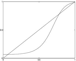
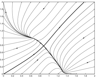
Figure 1: I/O characteristic and phase plane. Horizontal axis is $u$ (resp., $x_{1}$) and vertical axis is $x_{2}$.

(The value $\gamma=10$ was chosen only in order to help visualize the sigmoidal form of the characteristic, and similar results hold for a smaller and more biologically realistic constant.) As confirmed by a sketch of the phase plane, for almost all initial conditions, trajectories converge to the equilibria where the derivative condition is satisfied.

Of course, the interest of our results is in the high-dimensional case in which phase-plane techniques cannot provide the result, and we turn to such an example next. However, let us note that, for the special case of two-dimensional systems, our techniques are very close to those of [7]. In fact, even the 4-dimensional example of a two-repressor system with RNA dynamics, treated in [7] (Appendix I) in an ad-hoc manner, can be shown to be globally bistable as an immediate application of our techniques.

We now turn to a less trivial example where our tools may be applied. (A different example, involving cascades of systems of this type, and with comparisons with experimental data, is treated in [1].) Consider the following chemical reaction, involving various forms of a protein E:

$$\mbox{E}_{1}\;\;\raisebox{-4.30554pt}{$\stackrel{{\scriptstyle\stackrel{{\scriptstyle\mbox{\small U}}}{{\longrightarrow}}}}{{\stackrel{{\scriptstyle\longleftarrow}}{{}}}}$}\;\;\mbox{E}_{2}\;\;\raisebox{-4.30554pt}{$\stackrel{{\scriptstyle\stackrel{{\scriptstyle\mbox{\small U}}}{{\longrightarrow}}}}{{\stackrel{{\scriptstyle\longleftarrow}}{{}}}}$}\;\;\ldots\;\;\raisebox{-4.30554pt}{$\stackrel{{\scriptstyle\stackrel{{\scriptstyle\mbox{\small U}}}{{\longrightarrow}}}}{{\stackrel{{\scriptstyle\longleftarrow}}{{}}}}$}\;\;\mbox{E}_{n-1}\;\;\raisebox{-4.30554pt}{$\stackrel{{\scriptstyle\stackrel{{\scriptstyle\mbox{\small U}}}{{\longrightarrow}}}}{{\stackrel{{\scriptstyle\longleftarrow}}{{}}}}$}\;\;\mbox{E}_{n}$$

being driven forward by an enzyme U, with the different subscripts indicating an additional degree of phosphorylation, and with constitutive dephosphorylation. We will be interested in positive feedback from E_n to U.

A typical way to model such a reaction is as follows. We introduce variables $x_{i}(t)$, $i=1,\ldots,n$ to indicate the fractional concentrations of the various forms of the enzyme E (so that $x_{1}+\ldots+x_{n}\equiv 1$, and $x_{i}\geq 0$, for the solutions of physical interest), and $u(t)\geq 0$ to indicate the concentration of U. The differential equations are then as follows:

$$\dot{x}_{1} = -\sigma_{1}(u)\alpha_{1}(x_{1})+\beta_{2}(x_{2})$$

$$\dot{x}_{2} = \sigma_{1}(u)\alpha_{1}(x_{1})-\beta_{2}(x_{2})-\sigma_{2}(u)\alpha_{2}(x_{2})+\beta_{3}(x_{3})$$

$$\vdots$$

$$\dot{x}_{n-1} = \sigma_{n-2}(u)\alpha_{n-2}(x_{n-2})-\beta_{n-1}(x_{n-1})-\sigma_{n-1}(u)\alpha_{n-1}(x_{n-1})+\beta_{n}(x_{n})$$

$$\dot{x}_{n} = \sigma_{n-1}(u)\alpha_{n-1}(x_{n-1})-\beta_{n}(x_{n})\,.$$

We make the assumptions that $\alpha_{i}$ and $\beta_{i}$ (respectively, $\sigma_{i}$) are differentiable functions $[0,\infty)\rightarrow[0,\infty)$ with positive (respectively, either positive or identically zero) derivatives, and $\alpha_{i}(0)=\beta_{i}(0)=0$ and $\sigma_{i}(0)>0$ for each $i$. (We allow some of the $\sigma_{i}$ to be constant, and in this manner represent steps that are not controlled by U.) Since we are interested in studying the effect of feeding back E_n, we pick $y=x_{n}$.

Let us first prove that the characteristic is well-defined. As we said, we are only interested in the solutions that lie in the intersection $X$ of the plane $x_{1}+\ldots+x_{n}\equiv 1$ and the nonnegative orthant in ${\mathbb{R}}^{n}$. This set is easily seen to be invariant for the dynamics, and it is convex, so the Brower fixed point theorem guarantees the existence of an equilibrium in $X$, for any constant input $u(t)\equiv a$. We next prove that this steady-state is unique. Redefining if necessary the functions $\alpha_{i}$, we will assume without loss of generality that $\sigma_{i}(a)=1$ for all $i$. Let us introduce the nondecreasing functions

$$F_{k}\;=\;\beta_{k}^{-1}\circ\alpha_{k-1}\circ\beta_{k-1}^{-1}\circ\ldots\circ\beta_{2}^{-1}\circ\alpha_{1}$$

for each $k=2,\ldots,n$ and $F(r):=r+F_{2}(r)+\ldots+F_{n}(r)$. This function is defined on some maximal interval $[0,M]$, consisting of those $r$ such that $\alpha_{1}(r)$ belongs to the range of $\beta_{2}$, $\alpha_{2}(\beta_{2}^{-1}(\alpha_{1}(r)))$ belongs to the range of $\beta_{3}$, and so forth, and it is strictly increasing. Moreover, for each equilibrium $x=(x_{1},\ldots,x_{n})$, it holds that $x_{k}=F_{k}(x_{1})$, and therefore, recalling that $x_{1}+\ldots+x_{n}=1$, $F(x_{1})=1$. Thus, if $x$ and $\widetilde{x}$ are two steady states, we have $F(x_{1})=F(\widetilde{x}_{1})$. Since $F$ is strictly increasing, it follows that $x_{1}=\widetilde{x}_{1}$, and therefore that $x_{k}=F_{k}(x_{1})=F_{k}(\widetilde{x}_{1})=\widetilde{x}_{k}$ for all $k$, so uniqueness is shown.

We must prove stability. For that, we first perform a change of coordinates:

$$z_{1}=x_{1},\;z_{2}=x_{1}+x_{2},\;\ldots,\;z_{n-1}=x_{1}+\ldots+x_{n-1},\;z_{n}=x_{1}+\ldots+x_{n}$$

so that the equations in these new variables become (using that $\dot{z}_{k}=(d/dt)(x_{1}+\ldots+x_{k})$ and $x_{k}=z_{k}-z_{k-1}$ for $k>1$):

$$\dot{z}_{1} = -\sigma_{1}(u)\alpha_{1}(z_{1})+\beta_{2}(z_{2}-z_{1})$$

$$\vdots$$

$$\dot{z}_{k} = -\sigma_{k}(u)\alpha_{k}(z_{k}-z_{k-1})+\beta_{k+1}(z_{k+1}-z_{k})$$

$$\vdots$$

$$\dot{z}_{n-1} = -\sigma_{n-1}(u)\alpha_{n-1}(z_{n-1}-z_{n-2})+\beta_{n}(1-z_{n-1})$$

(and $z_{n}\equiv 1$). When the input $u(t)$ is equal to any given constant, the system described by the first $n-1$ differential equations, seen as evolving in the subset of ${\mathbb{R}}^{n-1}$ where $0\leq z_{1}\leq z_{2}\leq\ldots\leq z_{n-1}\leq 1$, is a tridiagonal strongly cooperative system, and thus a theorem due to Smillie (see [26]) insures that all trajectories converge to the set of equilibria. (The proof given in [28] is also valid when the state-space is closed, as here.) Moreover, linearizing at the equilibrium preserves the structure, so applying the same result to the linearized system we know that we have in fact an exponentially stable equilibrium. Thus, characteristics are well defined.

It is easy to verify from our graph conditions that the system (in the new coordinates) is monotone, since ${df_{i}}/{dz_{j}}>0$ for all pairs $i\not=j$, ${df_{i}}/{du}\leq 0$ for all $i$, and ${dh}/{dz_{i}}=0$ for all $i<n-1$ and ${dh}/{dz_{n-1}}<0$ (the output is $y=x_{n}=1-z_{n-1}$). Excitability and transparency need not hold at boundary points; however, Theorem 3 still applies, because the closed-loop system is strongly monotone. To see this, it is enough to show that every trajectory lies in the interior of $X$ for all $t>0$, since in the interior, the Jacobian matrices are irreducible. As the interior of $X$ is itself forward invariant (see e.g. [2]), it is sufficient to prove: for any $T>0$, if $F$ is the set of $t\in[0,T]$ such that $x(t)$ is in the boundary of $X$ (relative to the linear space $x_{1}+\ldots+x_{n}=1$), then $F\not=[0,T]$. Assume otherwise. For each $i$, consider the closed set $F_{i}=\{t\in[0,T]\;|\;x_{i}(t)=0\}$, and note that $\bigcup_{i}F_{i}=F$. If $F_{i}$ would be nowhere dense for every $i$, then their union $F$ would be nowhere dense, contradicting $F=[0,T]$. Thus there is some $i$ so that $F_{i}$ contains an open interval $(a,b)\subseteq[0,T]$. It follows that, for this $i$, $\dot{x}_{i}\equiv x_{i}\equiv 0$ on $(a,b)$, and (looking at the equations) this implies that $x_{i\pm 1}\equiv 0$ and, recursively, we obtain $x_{j}\equiv 0$ for all $j$, contradicting $x_{1}+\ldots+x_{n}=1$.

As a numerical example, let us pick $\sigma_{i}(r)=(0.01+r)/(1+r)$, $\alpha_{i}(r)=10\,r/(1+r)$, and $\beta_{i}(r)=r/(1+r)$ for all $i$, and $n=7$. (The constants have no biological significance, but the functional forms are standard models of saturation kinetics.) A plot of the characteristic is shown in Fig. 2(a). Since the intersection with the diagonal has three points as shown, we know that the closed-loop system (with $u=x_{n})$ will have two stable and one unstable equilibrium, and almost all trajectories converge to one of these two stable equilibria. To illustrate this convergence, we simulated six initial conditions, in each case with $x_{2}(0)=\ldots=x_{6}(0)=0$ and with the following choices of $x_{7}(0)$: 0.1, 0.2, 0.3, 0.4, 0.5, and 0.8 (and $x_{1}(0)=1-x_{7}(0)$). A plot of $x_{7}(t)$ for each of these initial conditions is shown in Fig. 2(b); note the convergence to the two predicted steady states.

Figure 2: Enzyme example: (a) Characteristic and (b) Simulations

9 External Stimuli, Thresholds and Hysteresis

Throughout this section we investigate the behavior of positive feedback interconnections of monotone systems which are in turn excited by some exogenous input. In particular we consider interconnections of the following type:

$$\begin{array}[]{rcl}\dot{x}&=&f(x,u,v)\\ y&=&h_{y}(x)\\ w&=&h_{w}(x)\end{array}$$ (30)

along with the unitary feedback interconnection $u=y$. The block diagram of such systems is shown in Fig. 3.

Figure 3: Block diagram of unitary feedback system with external inputs

We assume $f:X\times U\times V\rightarrow{\mathbb{R}}^{n}$ to be a locally Lipschitz function and that the system (30) is a monotone control system with input $[u,v]$ and output $[y,w]$ with respect to some ordering $\succeq_{x}$ of the state-space $X$ and cross-product orders as far as inputs $[u,v]$ and outputs $[y,w]$ are concerned, (i.e. $[u_{1},v_{1}]\succeq_{I}[u_{2},v_{2}]$ iff $u_{1}\succeq_{u}u_{2}$ and $v_{1}\succeq_{v}v_{2}$, $[y_{1},w_{1}]\succeq_{O}[y_{2},w_{2}]$ iff $y_{1}\succeq_{y}y_{2}$ and $w_{1}\succeq_{w}w_{2}$).

For each fixed value of the input $v$, systems as in (30) can be studied according to the techniques described previously.

A special instance of systems of this kind is given by single-input, single-output systems of the following form:

$$\begin{array}[]{rcl}\dot{x}&=&f(x,d)\\ d&=&g(v,y)\\ y&=&h(x)\end{array}$$ (31)

where $g:V\times U\rightarrow{\mathbb{R}}$ is a monotone and locally Lipschitz function (for instance $u,v\in{\mathbb{R}}_{\geq 0}$ and $g(v,y)=vy$ or $g(v,y)=v+y$). This structure (see Fig. 4) is of interest because it arises commonly in biological applications and is particularly suited for a graphical analysis.

Figure 4: A special feedback configuration of SISO systems

Next, we discuss the behavior of such interconnections in the presence of external stimuli. In particular, in the case of multistable systems we prove the existence of threshold values of inputs which trigger the transition among different equilibria.

The above considerations suggest the possibility of studying interconnections as in (30) by taking into account a parametrized family of I/O static characteristics in the $(u,y)$ plane, where the parameter is the exogenous input $v$. This type of analysis is very general and bifurcations can be traced by looking at the intersections of the parametrized I/O characteristic with the diagonal $u=y$. For the special structure (4) instead, the study can be carried out in the $(d,y)$-plane allowing some intuitive simplifications. A single I/O characteristic is needed in fact, from $d$ to $y$, and equilibria correspond to intersections with the “parametrized” family of functions $d=g(v,y)$, which also takes values in the $(d,y)$ plane. Although the analysis which follows is essentially a consequence of Theorem 3, it is still worth pursuing, because it provides a solid theoretical justification to phenomena which are well described and understood in many biological applications. Consider again the system (29), subject to the feedback interconnection $u=v\cdot y$. This results in the following set of equations:

$$\begin{array}[]{rcl}\dot{x}_{1}&=&\frac{\alpha_{1}}{1+(v\cdot x_{2})^{\beta}}-x_{1}\\ \dot{x}_{2}&=&\frac{\alpha_{2}}{1+x_{1}^{\gamma}}-x_{2}\\ y&=&x_{2}.\end{array}$$ (32)

We may therefore analyze the system by looking at the I/O static characteristic from $u$ to $y$, together with the $v$-parametrized family of lines $y=u/v$. Fig. 5 illustrates a typical situation, corresponding here to the parameters value in the following table:

$\gamma$	$6$	$\beta$	$3$
$\alpha_{1}$	$1.3$	$\alpha_{2}$	$1.3$

Notice that for $v=1$ bistability is obtained; in particular two equilibria are asymptotically stable and one is an unstable saddle whose stable manifold behaves as a separatrix for the basins of attractions of the stable equilibria. Bifurcations occur at two different values of $v$, approximately $v_{1}\approx 0.8$ and $v_{2}\approx 1.35$. This values correspond to the slopes of the tangent lines to the I/O characteristic. For all $v>v_{2}$ in fact there only exists one equilibrium, usually referred to as the activated equilibrium. For $v<v_{1}$ again only one equilibrium occurs but corresponding to a non-activated state. These values play therefore the role of input thresholds that may trigger transition from the non-activated state to an activated one and vice versa. After a signal of amplitude bigger than $v_{2}$ is applied for a sufficiently long time, the state will be in proximity of the activated equilibria. Then, this level of output will be maintained even after $v(t)$ drops below $v_{2}$, provided that $v_{1}<v(t)$. Further decrease of the $v(t)$ below $v_{1}$, for a sufficiently long time, will instead trigger transition to a deactivated state, which is afterward maintained also for higher values of $v(t)$, provided that $v(t)<v_{2}$. This kind of behavior, known as hysteresis, has been observed in many biological systems (see for instance [11], [23]). In an actual experimental situation, one would block the feedback of $x_{2}$, replacing the effect of $x_{2}$ by an experimentally set value of the input, and the bifurcation diagram would be obtained directly from the I/O characteristic, itself measured experimentally. See [1] for more discussion of this topic.

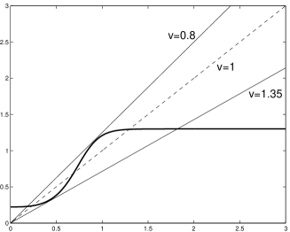
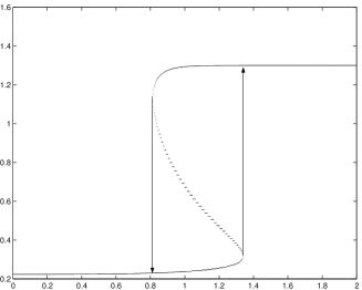
Figure 5: Thresholds and hysteresis; horizontal axis is $u$ (resp. $v$) and vertical axis is $x_{2}$.

10 Why is Monotonicity Imposed ?

Local analysis techniques based on the study of intersections of static characteristics of interconnected systems or, in the two-dimensional case of nullclines, are very common in mathematical biology. Our discussion shows that for the class of monotone systems, under relatively mild assumptions, almost global convergence results can be obtained and the investigation of the stability property of equilibria can be carried out just by graphical inspection at the intersection points of the I/O characteristics of systems in feedback. In this section we show by means of an example how monotonicity is a crucial assumption in this respect. The following planar system (a predator-prey system):

$$\begin{array}[]{rcl}\dot{x}_{1}&=&x_{1}(-x_{1}+x_{2})\\ \dot{x}_{2}&=&3x_{2}(-x_{1}+u)\\ y&=&c+b\frac{x_{2}^{4}}{k+x_{2}^{4}}\end{array}$$ (33)

evolving in ${\mathbb{R}}_{\geq 0}^{2}$, it is not monotone. However, it has a well defined (monotonically increasing) I/O static characteristic (see Fig. 6) provided that $c,b,k\in{\mathbb{R}}_{>0}$. Moreover, for certain parameters values, the I/O characteristics has $3$ (non-degenerate) fixed points. The closed-loop system resulting from the interconnection $u=y$, however, need not be globally converging at the set of equilibria. The simulations in Fig. 6 refer to the following values: $c=1.1,b=361/140,k=405/14$. Notice that the $3$ equilibria correspond to $2$ unstable foci and one saddle point.

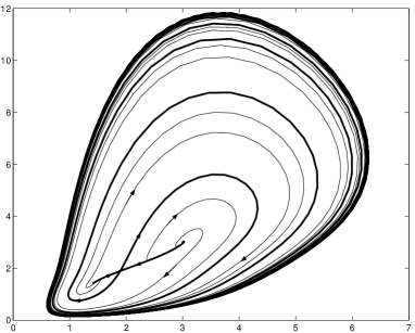
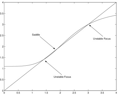
Figure 6: A stable limit cycle arising in a non-monotone feedback loop and the I/O static characteristic; horizontal axis is $x_{1}$ (resp. $u$) and vertical axis is $x_{2}$ (resp. $y$)

11 Conclusions

We have presented a general method for detecting multistability in a class of positive feedback systems. Our results apply when the original system has certain properties (well-defined characteristic, monotonicity). The results can be used in conjunction with other techniques being developed, such as the study of small-gain theorems for negative feedback interconnections (cf. [2]), in order to attempt to understand the behavior of complex biological signaling interconnections by first breaking up the system into smaller parts and then reconstituting the behavior of the entire system.

Appendix A Graphical characterizations of Transparency and Excitability

Lemma A.1

Consider a scalar differential equation $\dot{x}=f(x,u)$, evolving on a open subset of ${\mathbb{R}}$, where $u=(u_{1},u_{2},\ldots,u_{k})$ is a vector of input functions $u_{j}$ taking values in nonempty sets $U_{j}\subseteq{\mathbb{R}}$. We assume that $f$ is $C^{1}$ and that solutions are defined for all initial states and all $t>0$, for any locally bounded inputs. Suppose that the system is cooperative, that is, $f(x,u)$ is nondecreasing as a function of $u_{j}$, for all $j$ (meaning that, for every $x$, $f(x,u)\geq f(x,v)$ if $u_{j}\geq v_{j}$ for all $j$). Define the following set of indices:

$$I_{+}:=\left\{j^{\star}\in\{1,\ldots,k\}\;|\;f(x,u)\mbox{\ is strictly increasing as a function of\ }u_{j^{\star}}\right\}$$

(the strict increase condition meaning that $f(x,u)>f(x,v)$ for all $x,u,v$ such that $u_{j}\geq v_{j}$ for all $j$ and $u_{j^{\star}}>v_{j^{\star}}$), and, for each $j\in\{1,\ldots,k\}$, each $\varepsilon>0$, and each pair of inputs $u(\cdot)$ and $v(\cdot)$, the set of times:

$$S_{j,\varepsilon,u,v}:=\left\{t\in[0,\varepsilon]\;|\;u_{j}(t)>v_{j}(t)\right\}$$

(possibly empty). Pick any two inputs $u(\cdot)$ and $v(\cdot)$ such that $u\succeq v$ (i.e, $u_{j}(t)\geq v_{j}(t)$ for all $t$ and all $j$) and suppose that either:

1. there is some $j^{\star}\in I_{+}$ is such that the Lebesgue measure $\mu\left(S_{j^{\star},\varepsilon,u,v}\right)>0$ for each $\varepsilon>0$, or

2. $u\succ v$ and $I_{+}=\{1,\ldots,k\}$.

Then, for each initial state $\xi$, the respective solutions for these two inputs satisfy $x(t,\xi,u)>x(t,\xi,v)$ for all $t>0$.

Proof. Take two such inputs and initial state. Since the system is monotone, we know that $x(t,\xi,u)\geq x(t,\xi,v)$ for all $t>0$, but we need to prove that the strict inequality holds for all $t$. So suppose that there is some $T>0$ such that $x(T,\xi,u)=x(T,\xi,v)=\zeta$.

We claim that, then, $x(s,\xi,u)=x(s,\xi,v)$ for all $s<T$. This fact is an easy consequence of comparison arguments based upon monotonicity (see [24]). We provide a proof here for the reader’s convenience. Suppose that $\xi^{\prime}=x(S,\xi,u)>x(S,\xi,v)=\xi^{\prime\prime}$ for some $S<T$, and consider the following system of two differential equations:

$$\dot{x} = f(x,u)$$

$$\dot{z} = f(z,v)\,.$$

Pick a sequence $(a_{k},b_{k})\rightarrow(\zeta,\zeta)$ with the property that $a_{k}<b_{k}$ for all $k$ (for instance, $b_{k}\equiv\zeta$ and $a_{k}=\zeta-1/k$ for $k$ large enough). Let $\Phi$ be the map that sends initial states $(x(S),z(S))$ at time $S$ into states $(x(T,x(S),u_{S}),z(T,z(S),v_{S}))$ at time $T$, where $u_{S}$ and $v_{S}$ are the inputs restricted to times $\geq S$ (we may think of $\Phi$ as the time $T-S$ flow of the two-dimensional system). As this map is a diffeomorphism, there exists a sequence $(c_{k},d_{k})\rightarrow(\xi^{\prime},\xi^{\prime\prime})$ such that $\Phi(c_{k},d_{k})=(a_{k},b_{k})$ for all $k$. Since $\xi^{\prime}>\xi^{\prime\prime}$, it follows that $c_{k}>d_{k}$ for some $k$. This means that the solution of the above system, with initial state $x(S)=c_{k}>d_{k}=z(S)$ satisfies $x(T)<z(T)$, contradicting the monotonicity of the original system.

Since $x(s)=x(s,\xi,u)=x(s,\xi,v)$ for all $s<T$, we may take derivatives with respect to time to conclude that

$$f(x(s),u(s))=f(x(s),v(s))$$

for all $s\in[0,T]$.

Suppose that there is some $j^{\star}\in I_{+}$ so that $\mu\left(S_{j^{\star},T,u,v}\right)>0$. Then we may pick a time $t\in S_{T}$ so that $u_{j^{\star}}(t)>v_{j^{\star}}(t)$ and also $f(x(t),u(t))=f(x(t),v(t))$. This contradicts the strict increase assumption $j^{\star}\in I_{+}$.

Suppose instead that $u\succ v$. Then, we claim, there is some $j^{\star}$ such that $\mu\left(S_{j^{\star},\varepsilon,u,v}\right)>0$ for all $\varepsilon>0$. Indeed, if this claim were false, then there would be for each $j$ some $\varepsilon_{j}>0$ such that $\mu\left(S_{j,\varepsilon_{j},u,v}\right)=0$, which implies that also $\mu\left(S_{j,\varepsilon,u,v}\right)=0$, where $\varepsilon=\min\varepsilon_{j}$. Thus the union of these sets has measure zero, that is, $u_{j}(t)=v_{j}(t)$ for all $j$ and all $t\in[0,\varepsilon]$, contradicting $u\succ v$. Since $j^{\star}\in\{1,\ldots,m\}=I_{+}$, we have reduced to the first case.  

For one-dimensional systems, Theorem 4 can be strengthened into a necessary and sufficient statement. The proof of the Theorem will recursively use this result.

Corollary A.2

Let $\dot{x}=f(x,u)$ be a scalar cooperative system as in Lemma A.1, and assume that this system has a well-defined incidence graph. Then, the system is excitable if and only if $I_{+}=\{1,\ldots,k\}$, and it is weakly excitable if and only if $I_{+}\not=\emptyset$

Proof. Suppose that $I_{+}=\{1,\ldots,k\}$, and pick any two inputs $u\succ v$. The second case in the Lemma then gives that $x(t,\xi,u)>x(t,\xi,v)$ for all $t>0$, and this proves excitability. If, instead, $u\gg v$ and we know that $I_{+}\not=\emptyset$, we pick any $j^{\star}\in I_{+}$ and use the fact that $u\gg v$ implies that $S_{j^{\star},\varepsilon,u,v}=[0,\varepsilon]$ for all $\varepsilon$, so the first case in the Lemma then gives that $x(t,\xi,u)>x(t,\xi,v)$ for all $t>0$, and this proves weak excitability.

To prove the converse implications, we first consider the case $I_{+}=\emptyset$. By definition of incidence graph, this means that $\frac{\partial f}{\partial u_{j}}(x,u)\equiv 0$ for all $j$. Thus, solutions do not depend on input signals, and this contradicts weak excitability. If, instead, we only know that some $j^{\star}\not\in I_{+}$, then we have that $\frac{\partial f}{\partial u_{j^{\star}}}(x,u)\equiv 0$, and we may take any initial state $\xi$, and any two inputs $u(\cdot)$ and $v(\cdot)$ with the property that $u_{\ell}(t)=v_{\ell}(t)$ for all $t$ and all $\ell\not=j^{\star}$, and $u_{j^{\star}}(t)>v_{j^{\star}}(t)$; since $x(\cdot,\xi,u)\equiv x(\cdot,\xi,v)$, we have that $u\succ v$ but it is false that $x(t,\xi,u)>x(t,\xi,v)$ for $t>0$, contradicting excitability.  

Proof of Theorem 4

By appropriate coordinate changes $x_{i}\mapsto(-1)^{\delta_{i}}x_{i}$, as done in [2], one may restrict attention to cooperative systems.

Consider a cooperative system which admits an incidence graph and assume that each vertex $x_{i}$ is reachable from some input vertex $u_{j}$. Let $\xi$ be an arbitrary initial condition and let $u$, $v$ be arbitrary input signals satisfying $v\gg u$. We know that $x(t,\xi,v)\succeq x(t,\xi,u)$ for all $t$, and must show the strict inequality for all state components, i.e., $x(t,\xi,v)\gg x(t,\xi,u)$. We will prove this by induction, exploiting repeatedly Lemma A.1. To this end, we decompose the system in sublayers, based on the following notion of distance among vertices of a graph:

$$d(v\rightarrow w)=\min\{L(\mathcal{P}):\mathcal{P}_{0}=v\textrm{ and }\mathcal{P}_{L}=w\},$$ (34)

i.e. $d(v\rightarrow w)$ denotes the shortest length among all paths which link $v$ to $w$. Furthermore, for each state vertex $x_{i}$ of the incidence graph, we define the following integer:

$$D(x_{i})=\inf_{j}\;d(u_{j}\rightarrow x_{i})$$ (35)

(in words: $D(x_{i})$ corresponds to the minimum distance from some input vertex $u_{j}$ to the state vertex $x_{i}$). Notice, by the reachability assumption, that $D(x_{i})$ is well-defined ($<+\infty$) for every $i\in\{1,\ldots n\}$. We say that $x_{i}$ belongs to the $k$-th sublayer, if $D(x_{i})=k$.

Consider any state coordinate $x_{i}$ so that $D(x_{i})=1$ (such a coordinate always exists). We view $\dot{x}_{i}=f_{i}(x,u)$ as a scalar (cooperative) system, forced by the inputs $u$ and $x_{k}$ for all $k\neq i$. As $D(x_{i})=1$, there exists $j^{\star}$ such that $f_{i}(x,u)$ is strictly monotone as a function of $u_{j^{\star}}$. Since $u\gg v$, $v_{j^{\star}}(t)>u_{j^{\star}}(t)$ for almost all $t\geq 0$. Then the first part of Lemma A.1 allows us to conclude that $x_{i}(t,\xi,v)>x_{i}(t,\xi,u)$ for all $t>0$. This shows that the strict inequality holds for all state components belonging to the first sublayer.

Proceeding by induction, any component belonging to the $i$-th sublayer is reachable in one step from at least some component $x_{j}$ belonging to the $(i-1)$st sublayer (strict monotonicity of $f_{i}(x,u)$ with respect to $x_{j}$), and once again viewing $\dot{x}_{i}=f_{i}(x,u)$ as a scalar (cooperative) system, this time using $x_{j}(t)$ as the input, we conclude that $x_{i}(t,\xi,v)>x_{i}(t,\xi,u)$ for all $t>0$.

This completes the proof for the case of weak excitability. Next we consider the case of excitability.

Assume that $v\succ u$. Arguing as in the proof of Lemma A.1, we know that there exists an integer $j^{\star}$ so that $\mu\left(S_{j^{\star},\varepsilon,u,v}\right)>0$ for each $\varepsilon>0$. We again prove the result by induction by considering a sublayer decomposition, this time taken by looking at graph distances with respect to this particular input vertex $j^{\star}$, i.e.: $D(x_{i}):=d(u_{j^{\star}}\rightarrow x_{i})$. By the reachability assumption in the case of weak excitability, $D(x_{i})$ is well-defined for all $i\in\{1,2,\ldots n\}$.

Pick any state component $x_{i}$ for which $D(x_{i})=1$. Once again, we view $\dot{x}_{i}=f_{i}(x,u)$ as a scalar cooperative system, forced by the inputs $u$ and $x_{k}$ for all $k\neq i$. In particular $f_{i}(x,u)$ is strictly monotone with respect to $u_{j^{\star}}$, and we may apply the Lemma. Arguing by induction, any component belonging to the $i$-th sublayer is reachable in one step by some component belonging to the $(i-1)$st sublayer, and therefore a similar argument applies, yielding $x_{i}(t,\xi,v)>x_{i}(t,\xi,u)$ for all $t>0$.  

Sketch of Proof of Theorem 5

Consider an arbitrary pair of ordered initial conditions $\xi_{1}\succ\xi_{2}$. By monotonicity and uniqueness of solutions, we have $x(t,\xi_{1},u)\succ x(t,\xi_{2},u)$ for all $t\geq 0$. Arguing as earlier, we know that there must exist some index $j^{\star}$ so that, for all $\varepsilon>0$, the set $\{t\in[0,\varepsilon]\;|\;x_{j^{\star}}(t,\xi_{1},u)>x_{j^{\star}}(t,\xi_{2},u)\}$ has non-zero measure.

We claim that $x_{i}(t,\xi_{1},u)>x_{i}(t,\xi_{2},u)$ for every vertex $x_{i}$ which is reachable from the vertex $x_{j^{\star}}$, and denote with $\mathcal{R}_{j^{\star}}$ the set of such $x_{i}$s. The claim can be shown inductively by an argument analogous to the one employed in the proof of Theorem 4.

By the graph reachability condition (either weak or strong), for all (some) output vertices $y_{j}$ there exists at least one $x_{i}\in\mathcal{R}_{j^{\star}}$ so that $x_{i}\rightarrow y_{j}$ is an edge of the incidence graph. Thus, $h_{j}(x(t,\xi_{1},u))>h_{j}(x(t,\xi_{2},u))$ for all $t>0$ for all such $j$s.  

Appendix B Proof of Lemma 6.2

Proof. Consider the exponential map $\xi\rightarrow e^{At}\xi$. By positive invariance of $K$, for each $t>0$ the exponential is a linear map from $K$ to $K$. Moreover, for $t$ sufficiently small $t$, $t\rightarrow e^{\lambda}t$ is one-to-one on the spectrum of $A$. Thus, by Lemma A.3.3 in [30], the geometric multiplicity of $e^{\lambda_{i}t}$ as an eigenvalue of the exponential map is the same as that of $\lambda_{i}$ as an eigenvalue of $A$, with the same respective eigenvectors. Therefore, we can study the spectrum of $A$ by looking at the spectrum of its exponential map for $t$ sufficiently small. By the Perron-Frobenius Theorem, there exists a real positive eigenvalue $\mu$, with eigenvector $v\in K$, which is dominant in the sense that $\mu=\rho(e^{At})$ (eigenvalue of maximum modulus). Therefore, we conclude that $\lambda:=\log(\mu)/t$ is an eigenvalue for $A$, relative to the same eigenvector $v\in K$, and $\textrm{Re}(\lambda)\geq\textrm{Re}(\lambda_{i})$ for all $\lambda_{i}\in\textrm{Spec}(A)$.

References

- [1] D. Angeli, J. Ferrell, and E.D. Sontag, “Detection of multi-stability, bifurcations, and hysteresis in a large class of biological positive-feedback systems,” submitted.
- [2] D. Angeli and E.D. Sontag, “Monotone control systems,” IEEE Trans. Autom. Control, to appear. (Summarized version appeared as “A remark on monotone control systems,” in Proc. IEEE Conf. Decision and Control, Las Vegas, Dec. 2002, IEEE Publications, Piscataway, NJ, 2002, pp. 1876-1881.)
- [3] A. Berman and R.J. Plemmons, Nonnegative Matrices in the Mathematical Sciences, Academic Press, New York, 1979.
- [4] U.S. Bhalla and R. Iyengar, “Emergent properties of networks of biological signaling pathways”, Science 283(1999), pp. 381-387.
- [5] M. Delbrück, “Génétique du bactériophage,” in Unités Biologiques Douées de Continuité Génétique. Colloques Internationaux du Centre National de la Recherche Scientifique, vol. 8, CNRS, Paris, 1949, pp. 91-103.
- [6] R. de la Llave and C.E. Wayne, “On Irwin’s proof of the pseudostable manifold theorem,” Math. Z. 219(1995), pp. 301-321.
- [7] J.L. Cherry and F.R. Adler, “How to make a biological switch,” J. Theor. Biol. 203(2000): 117–133.
- [8] O. Cinquin and Demongeot J., “Positive and negative feedback: striking a balance between necessary antagonists,” J. Theor. Biol. 216(2002), pp. 229- 241
- [9] J.C. Doyle, B. Francis, and A. Tannenbaum, Feedback Control Theory, MacMillan publishing Co., Hampshire, England, 1990.
- [10] L. Farina and S. Rinaldi, Positive Linear Systems, Wiley-Interscience, Hoboken, NJ, 2000.
- [11] J.E. Ferrell and E.M. Machleder, “The biochemical basis of an all-r-none cell fate switch in Xenopus Oocytes”, Science Reports 280(1988), pp. 895-898.
- [12] J.E. Ferrell and Wen Xiong, “Bistability in cell signaling: How to make continuous processes discontinuous, and reversible processes irreversible,” Chaos 11(2001), pp. 227-236.
- [13] T.S. Gardner, C.R. Cantor and J.J. Collins, “Construction of a genetic toggle switch in Escherichia coli,” Nature 403(2000), pp. 339-342.
- [14] J.L. Gouzé, “Positive and negative circuits in dynamical systems,” J. Biol. Sys. 6(1998), pp. 11-15
- [15] A. Hunding and R. Engelhardt, “Early biological morphogenesis and nonlinear dynamics,” Journal of Theoretical Biology 173(1995), pp. 401-413.
- [16] M.W. Hirsch, “Systems of differential equations that are competitive or cooperative II: Convergence almost everywhere,” SIAM J. Mathematical Analysis 16(1985), pp. 423-439.
- [17] M.W. Hirsch, “Stability and convergence in strongly monotone dynamical systems,” Reine Angew. Math. 383(1988), pp. 1-53.
- [18] H. Kunze and D. Siegel, “A graph theoretical approach to monotonicity with respect to initial conditions”, in Comparison Methods and Stability Theory (Xinzhi Liu and David Siegel, eds.), Marcel Dekker, NY, 1994.
- [19] M. Laurent and N. Kellershohn, “Multistability: a major means of differentiation and evolution in biological systems,” Trends in Biochemical Sciences 24(1999), pp. 418-422.
- [20] A.S. Lewis, J.M. Borwein, Convex Analysis and Nonlinear Optimization: Theory and Examples Springer Verlag, New York, 2000.
- [21] C. Piccardi and S. Rinaldi, “Excitability, stability and the sign of equilibria in cooperative systems”, Systems and Control Letters 46(2002), pp. 153-163.
- [22] E. Plahte, T. Mestl, and W.S. Omholt, “Feedback circuits, stability and multistationarity in dynamical systems,” J. Biol. Sys. 3(1995), pp. 409-413.
- [23] J.R. Pomerening, E.D. Sontag, and J.E. Ferrell, “Building a cell cycle oscillator: hysteresis and bistability in the activation of Cdc2,” Nature Cell Biology 5(2003), pp. 346–351.
- [24] N. Rouche, P. Habets and M. Laloy, Stability Theory by Liapunov’s Direct Method, Springer-Verlag, NY 1977.
- [25] S. Smale, “On the differential equations of species in competition,” Journal of Mathematical Biology 3(1976), pp. 5–7.
- [26] J. Smillie, “Competitive and cooperative tridiagonal systems of differential equations,” SIAM J. Math. Anal. 15(1984): pp. 530–534.
- [27] H.L. Smith, Monotone Dynamical Systems: an Introduction to the Theory of Competitive and Cooperative systems, Mathematical Surveys and Monographs, Vol. 41, American Mathematical Society, Ann Arbor, 1995.
- [28] H.L. Smith, “Periodic tridiagonal competitive and cooperatibe systems of differential equations,” SIAM J. Math. Anal.22(1991): 1102-1109.
- [29] E.H. Snoussi, “Necessary conditions for multistationarity and stable periodicity,” J. Biol. Sys. 6(1998), pp. 3-9.
- [30] E.D. Sontag, Mathematical Control Theory: Deterministic Finite Dimensional Systems, Second Edition, Springer-Verlag, NY, 1998.
- [31] R. Thomas, “On the relation between the logical structure of systems and their ability to generate multiple steady states or sustained oscillations,” Springer Series in Synergetics 9, Springer-Verlag, Berlin, 1981, pp. 180-193.