Simplicial Cohomology of Orbifolds

Abstract

For any orbifold ${\cal M}$, we explicitly construct a simplicial complex $S({\cal M})$ from a given triangulation of the ‘coarse’ underlying space together with the local isotropy groups of ${\cal M}$. We prove that, for any local system on ${\cal M}$, this complex $S({\cal M})$ has the same cohomology as ${\cal M}$. The use of $S({\cal M})$ in explicit calculations is illustrated in the example of the ‘teardrop’ orbifold.

Introduction.

Orbifolds or V-manifolds were first introduced by Satake [9], and arise naturally in many ways. For example, the orbit space of any proper action by a (discrete) group on a manifold has the structure of an orbifold; this applies in particular to moduli spaces. Furthermore, the orbit space of any almost free action by a compact Lie group has the structure of an orbifold, as does the leaf space of any foliation with compact leaves and finite holonomy. Examples of orbifolds are discussed in [3, 9, 11] and many others.

For an orbifold ${\cal M}$, one can define in a natural way a cohomology theory with coefficients in any local system on ${\cal M}$. This cohomology is not an invariant of the underlying (‘coarse’) space, but of the finer orbifold structure. If the orbifold is given as the orbit space $X/G$ of a group action as above, this cohomology is the equivariant sheaf cohomology of the group action. It agrees with the (ordinary) cohomology of the Borel construction $EG\times_{G}X$.

This cohomology is the most natural one for orbifolds. It fits in well with the notion of fundamental group described in [11], by the familiar ‘Hurewicz formula’ $H^{1}({\cal M},A)=\mbox{\rm Hom}(\pi_{1}({\cal M}),A)$ (where $A$ is any abelian group).

The purpose of this paper is to give a simplicial description of these cohomology groups, suitable for calculations. More precisely, using triangulations of singular spaces [4], we will associate to any orbifold ${\cal M}$, presented by an orbifold atlas as in [9], a simplicial set $S({\cal M})$. The construction of $S({\cal M})$ uses the simplices in a triangulation of the coarse underlying space $M$ of ${\cal M}$, as well as all the local isotropy groups. The construction will have the following property.

Theorem For any local system of coefficients ${\cal A}$ on the orbifold ${\cal M}$, there is a canonically associated local system $A$ on the simplicial set $S({\cal M})$, for which there is a natural isomorphism $H^{*}({\cal M},{\cal A})\cong H^{*}(S({\cal M}),A)$.

After reviewing some preliminary definitions, we will present our construction in Section 2 of this paper. The proof of the theorem will be based on the fact that the simplicial set $S({\cal M})$ associated to an orbifold ${\cal M}$ is also closely related to the representation of ${\cal M}$ by a groupoid $G({\cal M})$ suggested in [5]. In fact, our proof shows that $S({\cal M})$ has the same homotopy type as the classifying space of $G({\cal M})$.

Before giving the proof in Section 4, we will present an example of calculations based on the simplicial construction for the ‘teardrop’ orbifold. We believe that much more work should be done in this direction. In fact, the explicit description of the simplicial set in terms of an atlas for the orbifold, and the resulting description of the cohomology groups by generators and relations, makes it suitable for computer assisted calculations.

1 Preliminaries.

1.1 Basic definitions.

In this section we briefly review the basic definitions concerning orbifolds, or V-manifolds in the terminology of Satake (see [9, 10, 11]). Let $M$ be a paracompact Hausdorff space. An orbifold chart on $M$ is given by a connected open subset $\tilde{U}\subseteq{\mathbb{R}}^{n}$ for some integer $n\geq 0$, a finite group $G$ of $C^{\infty}$-automorphisms of $\tilde{U}$, and a map $\varphi\colon\tilde{U}\rightarrow M$, such that $\varphi$ is $G$-invariant ($\varphi\circ g=\varphi$ for all $g\in G$) and induces a homeomorphism of $\tilde{U}/G$ onto the open subset $U=\varphi(\tilde{U})\subseteq M$. An embedding $\lambda\colon(\tilde{U},G,\varphi)\hookrightarrow(\tilde{V},H,\psi)$ between two such charts is a smooth embedding $\varphi\colon\tilde{U}\hookrightarrow\tilde{V}$ with $\psi\circ\lambda=\varphi$. An orbifold atlas on $M$ is a family ${\cal U}=\{(\tilde{U},G,\varphi)\}$ of such charts, which cover $M$ and are locally compatible in the following sense: given any two charts $(\tilde{U},G,\varphi)$ for $U=\varphi(\tilde{U})\subseteq M$ and $(\tilde{V},H,\psi)$ for $V\subseteq M$, and a point $x\in U\cap V$, there exists an open neighborhood $W\subseteq U\cap V$ of $x$ and a chart $(\tilde{W},K,\chi)$ for $W$ such that there are embeddings $(\tilde{W},K,\chi)\hookrightarrow(\tilde{U},G,\varphi)$ and $(\tilde{W},K,\chi)\hookrightarrow(\tilde{V},H,\psi)$. Two such atlases are said to be equivalent if they have a common refinement. An orbifold (of dimension $n$) is such a space $M$ with an equivalence class of atlases ${\cal U}$. We will generally write ${\cal M}=(M,{\cal U})$ for the orbifold ${\cal M}$ represented by the space $M$ and a chosen atlas ${\cal U}$.

1.1.1 Remarks.

• For two embeddings $\lambda,\mu\colon(\tilde{U},G,\varphi)\rightrightarrows(\tilde{V},H,\psi)$ between charts, there exists a unique $h\in H$ such that $\mu=h\circ\lambda$. In particular, since each $g\in G$ can be viewed as an embedding of $(\tilde{U},G,\varphi)$ into itself, there exists for the two embeddings $\lambda$ and $\lambda\circ g$ a unique $h\in H$ with $\lambda\circ g=h\circ\lambda$. This $h$ will be denoted by $\lambda(g)$. In this way, every embedding $\lambda$ also induces an injective group homomorphism, (again denoted) $\lambda\colon G\rightarrow H$, with defining equation

  $$\lambda(g\cdot\tilde{x})=\lambda(g)\lambda(\tilde{x})\qquad\qquad(\tilde{x}\in\tilde{U}).$$

  Furthermore, if $h\in H$ is such that $\lambda(\tilde{U})\cap h\cdot\lambda(\tilde{U})\neq\emptyset$, then $h$ belongs to the image of this group homomorphism $\lambda\colon G\rightarrow H$, and hence $\lambda(\tilde{U})=h\cdot\lambda(\tilde{U})$. (This is proved in [9] for the codimension 2 case, and in [7] for the general case.)

• By the differentiable slice theorem for smooth group actions [6], any orbifold of dimension $n$ has an atlas consisting of ‘linear’ charts, i.e. charts of the form $(\tilde{U},G)$ where $G$ is a finite group of linear transformations and $\tilde{U}$ is an open ball in ${\mathbb{R}}^{n}$.

• If $(\tilde{U},G,\varphi)$ and $(\tilde{V},H,\psi)$ are two charts for the same orbifold structure on $M$, and $\tilde{U}$ is simply connected, then there exists an embedding $(\tilde{U},G,\varphi)\hookrightarrow(\tilde{V},H,\psi)$ whenever $U\subseteq V$, i.e. when $\varphi(\tilde{U})\subseteq\psi(\tilde{V})$ (see [10], footnote 2). In this paper we will take all charts to be simply connected.

• If $(\tilde{U},G,\varphi)$ is a chart, and $V$ is a connected (and simply connected) open subset of $U\subseteq M$, then $V$ inherits a chart structure from $U$ in the following way: let $\tilde{V}$ be a connected component of $\varphi^{-1}(V)\subseteq\tilde{U}$, and let $H=\{g\in G|\,g\cdot\tilde{V}=\tilde{V}\}$. Then $(\tilde{V},H,\varphi|_{\tilde{V}})$ is a chart, which embeds into $(\tilde{U},G,\varphi)$, and hence defines the same orbifold structure on points in $V$.

1.1.2 Examples.

We list some well-known examples, see e.g. [5, 7, 11].

• If a discrete group $\Gamma$ acts smoothly and properly on a manifold $N$, the orbit space $M=N/\Gamma$ has a natural orbifold structure. Examples are weighted projective space and moduli spaces.

• If a compact Lie group $L$ acts smoothly on a manifold $N$ and the isotropy group $L_{x}$ at each point $x\in N$ is finite and acts faithfully on a slice $S_{x}$ through $x$, then the orbit space $N/L$ has a natural orbifold structure. Moreover any orbifold can be represented this way.

• If $N$ is a manifold equipped with a foliation ${\cal F}$ of codimension $n$, with the property that each leaf is compact and the holonomy group at each point is finite, then the space of leaves $N/{\cal F}$ has the natural structure of an $n$-dimensional orbifold. Again, any orbifold can be represented in this way.

1.2 Triangulation of orbifolds.

Let ${\cal M}=(M,{\cal U})$ be an orbifold of dimension $n$. For each point $x\in M$, one can choose a linear chart $(\tilde{U},G,\varphi)$ around $x$, with $G$ a finite subgroup of the linear group $\mbox{\rm Gl}(n,{\mathbb{R}})$. Let $\tilde{x}\in\tilde{U}$ be a point with $\varphi(\tilde{x})=x$, and $G_{x}=\{g\in G|\,g\cdot\tilde{x}=\tilde{x}\}$ the isotropy subgroup at $\tilde{x}$. Up to conjugation, $G_{x}$ is a well defined subgroup of $\mbox{\rm Gl}(n,{\mathbb{R}})$. The space $M$ thus carries a well-known natural stratification, whose strata are the connected components of the sets

$$S_{H}=\{x\in M|\,(G_{x})=(H)\},$$

where $H$ is any finite subgroup of $\mbox{\rm Gl}(n,{\mathbb{R}})$ and $(H)$ is its conjugacy class. It is also well-known ([12, 4]) that there exists a triangulation ${\cal T}$ of $M$ subordinate to this stratification (i.e. the closures of the strata lie on subcomplexes of the triangulation ${\cal T}$). By replacing ${\cal T}$ by a stellar subdivision, one can assume that the cover of closed simplices in ${\cal T}$ refines the atlas ${\cal U}$. For a simplex in such a triangulation, the isotropy groups of all interior points of $\sigma$ are the same, and are subgroups of the isotropy groups of the boundary points. By taking a further subdivision of ${\cal T}$, we may in fact assume that there is one face $\sigma^{\prime}\subset\sigma$ such that the isotropy is constant on $\sigma-\sigma^{\prime}$, and possibly larger on $\sigma^{\prime}$. In particular, any simplex $\sigma$ will then have a vertex $v\in\sigma$ with maximal isotropy, i.e. $G_{x}\subseteq G_{v}$ for all $x\in\sigma$. We call such a triangulation adapted to ${\cal U}$. For reference we state:

Proposition 1.2.1

For any orbifold $M$ and any orbifold atlas ${\cal U}$ there exists an adapted triangulation ${\cal T}$ for ${\cal M}=(M,{\cal U})$.

Let $\sigma$ be a (closed) $n$-simplex in such a triangulation, which is contained in a chart $U$. (In this paper we will take all simplices to be closed.) The next lemma describes how to lift $\sigma$ to a simplex $\tilde{\sigma}$ in $\tilde{U}$ by choosing a connected component of the inverse image $\varphi^{-1}(\mathord{\mathop{\sigma}\limits^{\smash{\circ}}})$ of the interior.

Lemma 1.2.2

For every connected component $S$ of the inverse image $\varphi^{-1}(\mathord{\mathop{\sigma}\limits^{\smash{\circ}}})$ of the interior of $\sigma$, the map $\varphi$ restricts to a homeomorphism on the closures $\varphi|_{\overline{S}}\,\colon\overline{S}\stackrel{{\scriptstyle\sim}}{{\longrightarrow}}\overline{\sigma}=\sigma$; in particular the triangulation of ${\sigma}$ lifts to a triangulation of $\overline{S}$.

Proof.

As is well-known (see e.g. [12, Lemma 1]), the map $\varphi\colon\tilde{U}\rightarrow\tilde{U}/G=U$ restricts to a covering projection on each stratum. In particular, since the isotropy is constant on the interior $\mathord{\mathop{\sigma}\limits^{\smash{\circ}}}$, we find that $\varphi^{-1}(\mathord{\mathop{\sigma}\limits^{\smash{\circ}}})=\coprod S_{i}$ is a disjoint sum of open simplices $S_{i}$ with $\varphi\colon S_{i}\stackrel{{\scriptstyle\sim}}{{\longrightarrow}}\mathord{\mathop{\sigma}\limits^{\smash{\circ}}}$. Let $S$ be one of these $S_{i}$. By continuity, $\varphi$ maps $\overline{S}$ to ${\sigma}$. This restriction is also surjective, because ${\sigma}\subseteq U$ and the action of $G$ on $\tilde{U}$ is continuous. Since ${\cal T}$ is subordinate to the stratification, the isotropy groups of the boundary points of $\sigma$ contain the isotropy group of the interior points, and therefore $\varphi$ has to be one-one on $\overline{S}$. Since $\varphi$ is also open (as quotient map), it follows that $\varphi|_{\overline{S}}\,\colon\overline{S}\stackrel{{\scriptstyle\sim}}{{\longrightarrow}}{\sigma}$.

By taking further stellar subdivisions of ${\cal T}$, we may assume that for every simplex $\sigma$ in ${\cal T}$, the closure of the open star

$$\mbox{\rm St}(\sigma)=\cup\{\mathord{\mathop{\tau}\limits^{\smash{\circ}}}|\sigma\subseteq\tau\}$$

is contained in a chart of the atlas ${\cal U}$. We will call a triangulation of ${\cal M}$ with these properties a good triangulation for ${\cal M}=(M,{\cal U})$.

Proposition 1.2.3

For any orbifold $M$ and any orbifold atlas ${\cal U}$ there exists a good triangulation ${\cal T}$ for ${\cal M}=(M,{\cal U})$.

Consider such a good triangulation. Let $x$ be a point of $M$, let $\sigma(x)$ be the smallest simplex containing $x$, and consider the open star neighborhood $\Sigma_{x}=\mbox{\rm St}(\sigma(x))$. Let $(\tilde{U},G,\varphi)$ be a chart in the atlas ${\cal U}$ for which $\overline{\mbox{\rm St}(\sigma(x))}\subset U=\varphi(\tilde{U})$. For later purposes, it is useful to describe how $\overline{\mbox{\rm St}(\sigma(x))}$ lifts to a triangulation in $\tilde{U}$.

Lemma 1.2.4

The closed star $\overline{\mbox{\rm St}(\sigma(x))}$ lifts to a triangulation ${\cal R}$ of

$$\varphi^{-1}(\overline{\mbox{\rm St}(\sigma(x))})\subseteq\tilde{U}$$

with the property that every connected component of $\varphi^{-1}({\mbox{\rm St}(\sigma(x))})$ contains precisely one lifting $\tilde{x}$ of $x$, and these components are open star neighborhoods $\Sigma_{\tilde{x}}=\mbox{\rm St}(\sigma(\tilde{x}))$ for the triangulation ${\cal R}$:

$$\varphi^{-1}(\Sigma_{x})=\coprod_{\tilde{x}\in\varphi^{-1}(x)}\Sigma_{\tilde{x}}.$$

Proof.

According to Lemma 1.2.2, for every $n$-simplex $\tau\in\overline{\mbox{\rm St}(\sigma(x))}$ and every connected component of $\varphi^{-1}(\mathord{\mathop{\tau}\limits^{\smash{\circ}}})$ there is precisely one lifting $\tilde{\tau}$ of $\tau$ containing that connected component. Since we could lift the whole triangulation of $\tau$ to $\tilde{\tau}$, we get together with $\tilde{\tau}$ also all its boundary simplices. Let ${\cal R}$ be the set of all those liftings (for all $n$-simplices in $\overline{\mbox{\rm St}(\sigma(x))}$ and their boundaries). It is clear that they cover $\varphi^{-1}(\overline{\mbox{\rm St}(\sigma(x))})$. Remark that for every simplex $\rho\in{\cal R}$, $\varphi|\rho$ becomes a homeomorphism onto a simplex in $\overline{\mbox{\rm St}(\sigma(x))}$. Let $\rho_{1},\rho_{2}\in{\cal R}$ be two simplices with $\rho_{1}\cap\rho_{2}\neq\emptyset$. Then $\varphi(\rho_{1}\cap\rho_{2})\subseteq\varphi(\rho_{1})\cap\varphi(\rho_{2})$. This last intersection is a simplex in ${\cal T}$, which we will denote by $\tau$. Let

$$\tilde{\tau}_{i}:=\varphi^{-1}(\varphi(\rho_{1})\cap\varphi(\rho_{2}))\cap\rho_{i}$$

be the two liftings of $\tau$ in the $\rho_{i}$. (Note that $\rho_{1}\cap\rho_{2}=\tilde{\tau}_{1}\cap\tilde{\tau}_{2}$.) There exists an element $g\in G$ such that $g\cdot\tilde{\tau}_{1}=\tilde{\tau}_{2}$. This element $g$ is in the isotropy group of $\varphi(\rho_{1}\cap\rho_{2})$, but not in the isotropy group of the rest of $\tau$. Since ${\cal T}$ is subordinate to the stratification induced by the isotropy groups, it follows that $\varphi(\rho_{1}\cap\rho_{2})$ is a subsimplex of $\tau$, and therefore a subsimplex of $\varphi(\rho_{1})$. We know already that $\varphi|\rho_{1}\colon\rho_{1}\stackrel{{\scriptstyle\sim}}{{\longrightarrow}}\varphi(\rho_{1})$, so $\rho_{1}\cap\rho_{2}=\varphi^{-1}(\varphi(\rho_{1}\cap\rho_{2}))\cap\rho_{1}$ is a simplex in ${\cal R}$.

Now consider two liftings $\tilde{x}$ and $g\cdot\tilde{x}$ of $x$ in $\tilde{U}$, and their open star neighborhoods $\Sigma_{\tilde{x}}$ and $\Sigma_{g\cdot\tilde{x}}$. Suppose $\Sigma_{\tilde{x}}\cap\Sigma_{g\cdot\tilde{x}}\neq\emptyset$, and let $y$ be a point in this intersection. Thus $y\in\mathord{\mathop{\tau}\limits^{\smash{\circ}}}$ where $\tilde{x}\in\tau$ and $g\cdot\tilde{x}\in\tau$. But $\varphi\colon\tilde{U}\rightarrow U$ is one-one on $\tau$, as shown in Lemma 1.2.2. So $\tilde{x}=g\cdot\tilde{x}$ and $\Sigma_{\tilde{x}}=\Sigma_{g\cdot\tilde{x}}$. This proves the lemma.

Corollary 1.2.5

Let ${\cal M}=(M,{\cal U})$ be any orbifold with atlas ${\cal U}$. There exists an atlas ${\cal V}$ for ${\cal M}$ such that

• ${\cal V}$ refines ${\cal U}$;

• For every chart $(\tilde{V},H,\psi)$ in ${\cal V}$, both $\tilde{V}$ and $V$ are contractible;

• The intersection of finitely many charts in ${\cal V}$ is either empty or again a chart in ${\cal V}$.

Proof.

For a good triangulation ${\cal T}$ of $(M,{\cal U})$ as above, consider a simplex $\sigma$. The open star $V=\mbox{\rm St}(\sigma)$ is contained in $U$ for some chart $(\tilde{U},G,\varphi)$ in ${\cal U}$. Let $x$ be a point in the interior of $\sigma$, so that $V=\Sigma_{x}$. Choose a lifting $\tilde{x}$ of $x$ in $\tilde{U}$. Then, by Lemma 1.2.4 and Remark 1.1.1(iv), the map $\varphi\colon\Sigma_{\tilde{x}}\rightarrow\Sigma_{x}$ is part of a chart for ${\cal M}$. The collection of all these charts for open stars $V=\mbox{\rm St}(\sigma)$ is the required atlas ${\cal V}$.

Following the terminology of [2, page 42], we call a cover ${\cal V}$ of ${M}$ by charts as in Proposition 1.2.5 a good cover of the orbifold ${\cal M}$.

1.3 Sheaf cohomology.

Let ${\cal M}=(M,{\cal U})$ be an orbifold. Recall ([7]) that a sheaf on ${\cal M}$ is given by the following data:

• For each chart $(\tilde{U},G,\varphi)$ in ${\cal U}$ an (ordinary) sheaf of abelian groups ${\cal A}_{\tilde{U}}$ on $\tilde{U}$;

• For each embedding

  $$\lambda\colon(\tilde{U},G,\varphi)\rightarrow(\tilde{V},H,\psi)$$

  an isomorphism

  $${\cal A}(\lambda)\colon{\cal A}_{\tilde{U}}\stackrel{{\scriptstyle\sim}}{{\longrightarrow}}\lambda^{*}({\cal A}_{\tilde{V}}).$$

  These isomorphisms are required to be functorial in $\lambda$; i.e. if

  $$\mu\colon(\tilde{V},H,\psi)\rightarrow(\tilde{W},K,\chi)$$

  is another embedding, then the following square commutes:

  where ‘=’ denotes the canonical isomorphism;

• It follows that each ${\cal A}_{\tilde{U}}$ is a $G$-equivariant sheaf on $\tilde{U}$, see [7].

With the obvious notion of morphisms between sheaves, these sheaves form an abelian category $\mbox{\it Ab}({\cal M})$ with enough injectives.

Referring to the examples in Section 1.1, we remark that if the orbifold is defined from the action of a compact Lie group $L$ on a manifold $N$, then this category is (equivalent to) the category of $L$-equivariant sheaves on $N$. And if the orbifold is defined from a suitable foliation ${\cal F}$ on a manifold $N$, it is (equivalent to) the category of holonomy-invariant sheaves on $N$.

For a sheaf ${\cal A}$ as above, a global section $s$ of ${\cal A}$ is by definition a system of sections $s_{\tilde{U}}\in\Gamma(\tilde{U},{\cal A}_{\tilde{U}})$, one for each chart $\tilde{U}$, and compatible in the sense that for each embedding $\lambda\colon\tilde{U}\rightarrow\tilde{V}$, the identity ${\cal A}(\lambda)(s_{\tilde{U}})=\lambda^{*}(s_{\tilde{V}})$ holds. The group of all these global sections is denoted $\Gamma({\cal M},{\cal A})$. This defines a functor $\Gamma\colon{\it Ab}({\cal M})\rightarrow{\it Ab}$, into the category of abelian groups, which is right exact and preserves injectives. For an abelian sheaf ${\cal A}$, one defines

$$H^{n}({\cal M},{\cal A})=(R^{n}\Gamma)({\cal A}).$$

This definition of the sheaf cohomology of ${\cal M}$ is just a special case of the cohomology of a topos [1], and hence it satisfies all the standard functoriality and invariance properties. By way of example, we mention some of these properties:

1.3.1 Standard properties.

• Any (strong, [7]) map between orbifolds $f\colon{\cal N}\rightarrow{\cal M}$ induces an exact functor $f^{*}\colon{\it Ab}({\cal M})\rightarrow{\it Ab}({\cal N})$, and an induced homomorphism $f^{*}\colon H^{n}({\cal M},{\cal A})\rightarrow H^{n}({\cal N},f^{*}{\cal A})$.

• There is also an (adjoint) functor $f_{*}\colon{\it Ab}({\cal N})\rightarrow{\it Ab}({\cal M})$ and a corresponding (‘Leray’) spectral sequence

  $$E^{p,q}_{2}=H^{p}({\cal M},R^{q}f_{*}({\cal B}))\Rightarrow H^{p+q}({\cal N},{\cal B})$$

  see [1, Exposé V, Section 5].

• There are adjoint functors

  $$\pi_{*}\colon{\it Ab}({\cal M})\leftrightarrows{\it Ab}(M)\,\colon\negthinspace\pi^{*},$$

  where ${\it Ab}(M)$ is the category of abelian sheaves on the underlying space $M$. There is a corresponding Leray spectral sequence

  $$E^{p,q}_{2}=H^{p}(M,R^{q}\pi_{*}({\cal A}))\Rightarrow H^{p+q}({\cal M},{\cal A}),$$

  where for a point $x\in M$, the stalk $R^{q}\pi_{*}({\cal A})_{x}$ is $H^{q}(G_{\tilde{x}},{\cal A}_{\tilde{x}})$. (Here ${\cal A}_{\tilde{x}}$ is the stalk of ${\cal A}_{\tilde{U}}$ at any lifting $\tilde{x}\in\tilde{U}$ of $x$ for some chart $(\tilde{U},G,\varphi)$, and the stabilizer $G_{\tilde{x}}$ acts on ${\cal A}_{\tilde{x}}$ since ${\cal A}_{\tilde{U}}$ is $G$-equivariant.

• (Mayer-Vietoris) If $M=U\cup V$ is a union of two open sets, the orbifold structure ${\cal M}$ restricts to orbifold structures ${\cal M}|U$ and ${\cal M}|V$, and there is a Mayer-Vietoris sequence

  $$\rightarrow H^{n}({\cal M}|U,{\cal A}|U)\oplus H^{n}({\cal M}|V,{\cal A}|V)\rightarrow H^{n}({\cal M}|U\cap V,{\cal A}|U\cap V)\rightarrow H^{n+1}({\cal M},{\cal A})\rightarrow$$

• Define a presheaf ${\cal H}^{q}({\cal A})$ on the underlying space $M$, by ${\cal H}^{q}({\cal A})(U)=H^{q}({\cal M}|U,{\cal A}|U)$. For any open cover ${\cal V}$ of $M$, there is a spectral sequence

  $$E^{p,q}_{2}=\check{H}^{p}({\cal V},{\cal H}^{q}({\cal A}))\Rightarrow H^{p+q}({\cal M,A})$$

  with as $E^{p,q}_{2}$-term the Čech cohomology of this cover ${\cal V}$ with coefficients in this presheaf ${\cal H}^{p}({\cal A})$; see [1, Exposé V, Section 3].

• We single out a special case of this last property (v). A sheaf on ${\cal M}$ is said to be locally constant if each of the (ordinary) sheaves ${\cal A}_{\tilde{U}}$ is locally constant. Now suppose ${\cal V}$ is a ‘good’ atlas for ${\cal M}$, as in Corollary 1.2.5, and let ${\cal A}$ be any locally constant sheaf. For any chart $(\tilde{V},H,\psi)$ in ${\cal V}$, the restriction ${\cal A}_{\tilde{V}}$ is a constant sheaf on a contractible space ${\tilde{V}}$, and $H^{q}({\cal M}|V,{\cal A}|V)$ is the cohomology of the group $G=G_{V}$ with coefficients in the $G_{V}$-module $A_{V}=\Gamma(\tilde{V},{\cal A}_{\tilde{V}})$. Thus, for a locally constant sheaf ${\cal A}$ and a good cover ${\cal V}$, the spectral sequence takes the form

  $$\check{H}^{p}({\cal V},V\mapsto{H}^{q}(G_{V},A_{V}))\Rightarrow H^{p+q}({\cal M,A}).$$

2 Simplicial complexes for orbifolds.

Our purpose in this section is to describe explicitly for any orbifold ${\cal M}=(M,{\cal U})$ a simplicial set $S$, with the property that any locally constant sheaf ${\cal A}$ on ${\cal M}$ induces a local system of coefficients $A$ on $S$ for which there is a natural isomorphism

$$H^{*}({\cal M,A})\cong H^{*}(S,A),$$

see Theorem 2.1.1 below.

2.1 The simplicial set.

Let us fix an $n$-dimensional orbifold ${\cal M}$ with underlying space $M$ and (chosen) atlas ${\cal U}$; let us also fix a triangulation ${\cal T}$ of ${\cal M}$, and write $S_{0}$ for the set of $n$-simplices. We assume that the triangulation is adapted to ${\cal U}$, as described in Section 1.2. Recall that this means that ${\cal T}$ has the following properties:

• For each $n$-simplex $\sigma\in S_{0}$ there is a chart $(\tilde{U}_{\sigma},G_{\sigma},\varphi_{\sigma})$, such that $\sigma\subseteq U_{\sigma}$;

• For each simplex $\tau$ there is a face $\tau^{\prime}\subseteq\tau$ such that the isotropy is constant on $\tau-\tau^{\prime}$; in particular every simplex has a vertex $v(\tau)$ with maximal isotropy.
  

We assume that a choice of charts $U_{\sigma}$ and vertices $v(\tau)$ as in (i) and (ii) above has been made. (Note that we do not require the stronger property of being ‘good’ for the triangulation, because in some examples that would force us to construct a simplicial complex which is bigger than necessary, and hence less suitable for calculations.)

We now construct the simplicial set $S=S({\cal T})$ with the same cohomology as ${\cal M}$. The description of $S$ will use various choices, besides the charts $U_{\sigma}$ and the vertices $v(\tau)$ already mentioned. First of all, choose for each simplex $\sigma\in S_{0}$ a lifting $\tilde{\sigma}$ as in Lemma 1.2.2, mapped homeomorphically to $\sigma\subseteq U_{\sigma}$ by $\varphi_{\sigma}\colon\tilde{U}_{\sigma}\rightarrow U_{\sigma}$. Next, fix for each vertex $v$ of ${\cal T}$ a neighborhood $U_{v}$ of $v$ and a chart $(\tilde{U}_{v},G_{v},\varphi_{v})$ over $U_{v}$, so small that $U_{v}\subseteq U_{\sigma}$ whenever $v\in\sigma\in S_{0}$. Also fix a lifting $\tilde{v}\in\varphi_{v}^{-1}(v)$, and an embedding $\lambda_{\sigma,v}\colon\tilde{U}_{v}\hookrightarrow\tilde{U}_{\sigma}$ with $\lambda_{\sigma,v}(\tilde{v})\in\tilde{\sigma}$.

We will not require these $U_{v}$ to belong to the original atlas ${\cal U}$. In fact, they can be chosen so small that $G_{v}$ is also the isotropy group of $v$ in the chart $(\tilde{U}_{v},G_{v},\varphi_{v})$, so that the notation is unambiguous; in this case the lifting $\tilde{v}$ is unique.

Let $\sigma_{0},\sigma_{1}\in S_{0}$ be two simplices of maximal dimension $n$, and assume $\sigma_{0}\cap\sigma_{1}\neq\emptyset$. Below, in Section 2.2, we will construct for any two simplices $\tau$ and $\rho$ with

$$\tau\subseteq\rho\subseteq\sigma_{0}\cap\sigma_{1}$$ (1)

an injective map

$$\mu_{\tau,\rho,\sigma_{0},\sigma_{1}}\colon G_{v(\tau)}\rightarrow G_{v(\rho)}.$$ (2)

We will write $\mu$ or $\mu_{\tau,\rho}$ if the (other) subscripts are clear from the context. This map $\mu$ in (2) will not be a homomorphism in general; it will map $G_{v(\tau)}$ to a coset of a conjugate of the subgroup $G_{v(\tau)}=\{g\in G_{v(\rho)}|\,g\cdot v(\tau)=v(\tau)\}$ in $G_{v(\rho)}$. However the construction will have the following multiplicative property: if

$$\tau\subseteq\rho\subseteq\sigma_{0}\cap\sigma_{1}\cap\sigma_{2}$$

then, for $h_{1},h_{2}\in G_{v(\tau)}$,

$$\mu_{\sigma_{0},\sigma_{1}}(h_{1})\cdot\mu_{\sigma_{1},\sigma_{2}}(h_{2})=\mu_{\sigma_{0},\sigma_{2}}(h_{1}h_{2}).$$ (3)

Moreover, if $\tau=\rho$ and $\sigma_{0}=\sigma_{1}$ then $\mu\colon G_{v(\tau)}\rightarrow G_{v(\tau)}$ is the identity.

With these choices made, the simplicial set $S=S({\cal T})$ can be described. As already defined above,

$$S_{0}=\{\sigma|\,\sigma\mbox{ is an $n$-simplex of }{\cal T}\}.$$

Furthermore, for $k\geq 1$,

$$S_{k}=\sum_{\stackrel{{\scriptstyle\scriptstyle\sigma_{0},\cdots,\sigma_{k}\in S_{0}}}{{\sigma_{0}\cap\cdots\cap\sigma_{k}\neq\emptyset}}}G^{k}_{v(\sigma_{0}\cap\cdots\cap\sigma_{k})}.$$

An element of $S_{k}$ can also be denoted by

$$\sigma_{0}\stackrel{{\scriptstyle g_{1}}}{{\leftarrow}}\sigma_{1}\leftarrow\cdots\stackrel{{\scriptstyle g_{k}}}{{\leftarrow}}\sigma_{k},$$ (4)

to suggest the analogy with nerves. So $\sigma_{0},\cdots,\sigma_{k}$ in (4) are $n$-simplices, and $g_{1},\cdots,g_{k}\in G_{v(\tau)}$ where $v(\tau)$ is the chosen vertex with maximal isotropy on $\tau=\sigma_{0}\cap\cdots\cap\sigma_{k}$. The degeneracy maps $s_{i}\colon S_{k-1}\rightarrow S_{k}$ $(i=0,\cdots,k-1)$ are defined in the usual way,

$$s_{i}(\sigma_{0}\stackrel{{\scriptstyle g_{1}}}{{\leftarrow}}\cdots\stackrel{{\scriptstyle g_{k-1}}}{{\leftarrow}}\sigma_{k-1})=(\sigma_{0}\stackrel{{\scriptstyle g_{1}}}{{\leftarrow}}\cdots\sigma_{i}\stackrel{{\scriptstyle 1}}{{\leftarrow}}\sigma_{i}\cdots\stackrel{{\scriptstyle g_{k-1}}}{{\leftarrow}}\sigma_{k-1}).$$

The face maps $d_{j}\colon S_{k}\rightarrow S_{k-1}$ $(j=0,\cdots,k)$ are defined by means of the maps $\mu$ in (2), as

$$d_{j}(\sigma_{0}\stackrel{{\scriptstyle g_{1}}}{{\longleftarrow}}\cdots\stackrel{{\scriptstyle g_{k}}}{{\longleftarrow}}\sigma_{k})=\negthinspace\left\{\begin{array}[]{ll}\negthinspace\negthinspace\negthinspace\sigma_{1}\stackrel{{\scriptstyle\mu(g_{2})}}{{\longleftarrow}}\sigma_{2}\longleftarrow\cdots\stackrel{{\scriptstyle\mu(g_{k})}}{{\longleftarrow}}\sigma_{k},&\negthinspace\negthinspace\negthinspace(j=0)\\ \negthinspace\negthinspace\negthinspace\sigma_{0}\stackrel{{\scriptstyle\mu(g_{1})}}{{\longleftarrow}}\cdots\sigma_{j-1}\stackrel{{\scriptstyle\mu(g_{j}g_{j+1})}}{{\longleftarrow}}\sigma_{j+1}\cdots\longleftarrow\sigma_{k},&\negthinspace\negthinspace\negthinspace(0<j<k)\\ \negthinspace\negthinspace\negthinspace\sigma_{0}\stackrel{{\scriptstyle\mu(g_{1})}}{{\longleftarrow}}\cdots\stackrel{{\scriptstyle\mu(g_{k-1})}}{{\longleftarrow}}\sigma_{k-1},&\negthinspace\negthinspace\negthinspace(j=k),\end{array}\right.$$

where the $\mu$’s carry the following subscripts. Write $\tau=\sigma_{0}\cap\cdots\cap\sigma_{k}$ and $\rho=\sigma_{0}\cap\cdots\hat{\sigma}_{j}\cap\cdots\cap\sigma_{k}$. Then

$$\mu(g_{j})=\mu_{\tau,\rho,\sigma_{j-1},\sigma_{j}}(g_{j})$$

and

$$\mu(g_{j}g_{j+1}) = \mu_{\tau,\rho,\sigma_{j-1},\sigma_{j+1}}(g_{j}g_{j+1})$$

$$= \mu_{\tau,\rho,\sigma_{j-1},\sigma_{j}}(g_{j})\mu_{\tau,\rho,\sigma_{j},\sigma_{j+1}}(g_{j+1}),$$

the latter by (3). The simplicial identities now follow easily.

Before we define these maps $\mu$, we state the theorem. Let ${\cal A}$ be a locally constant sheaf on ${\cal M}$. This sheaf induces in a natural way a local system of coefficients $A$ on the simplicial set $S_{\bullet}$, with, for any $\sigma\in S_{0}$,

$$A_{\sigma}=\Gamma(\tilde{\sigma},{\cal A}_{\tilde{U}_{\sigma}}).$$

To describe the twisting, observe that, since ${\cal A}$ is locally constant, ${\cal A}_{\tilde{U}_{\sigma}}$ is constant on $\tilde{\sigma}$. So for any vertex $\tilde{w}\in\tilde{\sigma}$ there is a canonical isomorphism from the stalk at $\tilde{w}$,

Modulo these isomorphisms, the twisting by an element $(\sigma_{0}\stackrel{{\scriptstyle g}}{{\leftarrow}}\sigma_{1})\in S_{1}$ is now defined as the dashed map in the diagram of maps between stalks

Here $v=v(\sigma_{0}\cap\sigma_{1})$, so $g\in G_{v}$. Furthermore, $\lambda_{i}=\lambda_{\sigma_{i},v}\colon\tilde{U}_{v}\rightarrow\tilde{U}_{\sigma_{i}}$ is the chosen embedding $(i=0,1)$, with the property that $\tilde{v}_{i}=\lambda(\tilde{v})\in\tilde{\sigma}_{i}$. Finally, $\overline{g}$ in the diagram denotes the left action by $g\in G_{\tilde{v}}$ (cf. condition (iii) in the description of sheaves in Section 1.3).

Theorem 2.1.1

For any triangulated orbifold ${\cal M}$ with associated simplicial set $S$ as above, and for any locally constant sheaf ${\cal A}$ on ${\cal M}$, there is a natural isomorphism

$$H^{\raisebox{0.8pt}{${\scriptscriptstyle\,\bullet}$}}({\cal M,A})\cong H^{\raisebox{0.8pt}{${\scriptscriptstyle\,\bullet}$}}(S,A).$$

We will now first define the maps $\mu$ involved in the definition of $S$. The proof of the theorem will be given in Section 4.3.

2.2 Construction of $\mu$.

Fix $\sigma_{0},\sigma_{1}\in S$ and $\tau\subseteq\rho\subseteq\sigma_{0}\cap\sigma_{1}$ as in (1). Write $v=v(\tau)$ and $w=v(\rho)$ for the corresponding vertices with maximal isotropy on $\tau$ and $\rho$, respectively. We will construct

$$\mu\colon G_{v}\rightarrow G_{w}.$$ (5)

Let $\theta$ be the 1-simplex joining $v$ and $w$ in $\rho$. Then the isotropy group of any interior point of $\theta$ agrees with that of $v$, while that of $w$ is possibly larger, $w$ being maximal on $\theta$. Recall that we have already chosen

$$\begin{array}[]{ll}\lambda_{i}=\lambda_{\sigma_{i},v}\colon\tilde{U}_{v}\rightarrow\tilde{U}_{\sigma_{i}},&\lambda_{i}(\tilde{v})\in\tilde{\sigma}_{i},\\ \chi_{i}=\lambda_{\sigma_{i},w}\colon\tilde{U}_{w}\rightarrow\tilde{U}_{\sigma_{i}},&\chi_{i}(\tilde{w})\in\tilde{\sigma}_{i}.\end{array}$$

First consider the special case that there is a chart $(\tilde{W},H,\psi)$ for a neighborhood $W\supseteq\theta$, for which $U_{v},U_{w}\subseteq W$ and $W\subseteq U_{\sigma_{0}}\cap U_{\sigma_{1}}$. (Such a chart exists, for example, when one starts with a ‘good’ atlas ${\cal U}$ as in Section 1.2, in which case one can take $W=U_{\sigma_{0}}\cap U_{\sigma_{1}}$.) Choose an embedding

$$\gamma_{0}\colon\tilde{W}\rightarrow\tilde{U}_{\sigma_{0}}$$

with $\gamma_{0}(\tilde{W})\cap\tilde{\sigma}_{0}\neq\emptyset$. Let $\tilde{\theta}=\gamma_{0}^{-1}(\tilde{\sigma}_{0}\cap\varphi_{\sigma_{0}}^{-1}(\theta))\subseteq\tilde{W}$ be a lifting of $\theta$, and choose the other embedding

$$\gamma_{1}\colon\tilde{W}\rightarrow\tilde{U}_{\sigma_{1}}$$

such that $\gamma_{1}(\tilde{\theta})\subseteq\tilde{\sigma}_{1}$. Also choose embeddings

$$\tilde{U}_{v}\stackrel{{\scriptstyle\alpha}}{{\longrightarrow}}\tilde{W}\stackrel{{\scriptstyle\beta}}{{\longleftarrow}}\tilde{U}_{w}$$

with $\alpha(\tilde{v}),\,\beta(\tilde{w})\in\tilde{\theta}$.

Now observe that, since $\gamma_{0}\alpha$ and $\lambda_{0}$ both map $\tilde{v}$ into $\tilde{\sigma}_{0}$, one has $\gamma_{0}\alpha(\tilde{v})=\lambda_{0}(\tilde{v})$, and hence there is a $g_{0}\in G_{v}$ such that $\gamma_{0}\alpha=\lambda_{0}g_{0}$ (cf. Section 1.1, Remark (i)). Similarly, we find $g_{1}\in G_{v}$ and $h_{0},h_{1}\in G_{w}$, such that

$$\gamma_{i}\alpha=\lambda_{i}g_{i},\quad\gamma_{i}\beta=\chi_{i}h_{i},\quad(i=0,1).$$

We claim that for any $k\in G_{v}$ there is a (unique) $m\in G_{w}$ such that

$$\alpha(g_{0}^{-1}kg_{1})=\beta(h_{0}^{-1}mh_{1}).$$ (6)

To see this, recall first that $H$ denotes the group of the chart $\tilde{W}$, and consider

$$\ell=\alpha(g_{0}^{-1}kg_{1}).$$

Note that $\ell$ fixes $\alpha(\tilde{v})\in\tilde{\theta}$. Since the isotropy along $\alpha(\tilde{\theta})$ does not decrease from $\alpha(\tilde{v})$, it follows that $\ell$ fixes $\tilde{\theta}$, and hence also the point $\beta(\tilde{w})$. Thus $\ell=\beta(\ell^{\prime})$ for some $\ell^{\prime}\in G_{w}$. Now let

$$m=h_{0}\ell^{\prime}h_{1}^{-1}.$$

Then $\alpha(g_{0}^{-1}kg_{1})=\beta(h_{0}^{-1}mh_{1})$, as required for (6).

We now define $\mu$ in (5) by

$$\mu(k)=m.$$ (7)

It can be shown that this definition is independent of the choices made above (of $\tilde{W}$, $\alpha$, $\beta$).

This defines $\mu$ in the special case, where the 1-simplex $\theta$ is contained in a chart $W$ with $U_{\sigma_{0}}\cap U_{\sigma_{1}}\supseteq W\supseteq U_{v},U_{w}$. In the general case, choose a subdivision of $\theta$ into smaller 1-simplices, with vertices

$$v=x_{0},\,x_{1},\cdots,\,x_{n}=w.$$

Choose charts

$$\tilde{U}_{v}=\tilde{U}_{x_{0}},\,\tilde{U}_{x_{1}},\cdots,\,\tilde{U}_{x_{n}}=\tilde{U}_{w},$$

liftings $\tilde{x}_{i}\in\tilde{U}_{x_{i}}$, and embeddings

$$\lambda_{x_{j},i}\colon\tilde{U}_{x_{j}}\rightarrow\tilde{U}_{\sigma_{i}}\quad(i=0,1;\,j=0,\cdots,n),$$

with $\lambda_{x_{j},i}(\tilde{x}_{j})\in\tilde{\sigma}_{i}$, and coinciding with the embeddings already chosen for $j=0,n$. Furthermore, choose this subdivision of $\theta$ sufficiently fine, and these charts $\tilde{U}_{x_{i}}$ sufficiently small, so that each 1-simplex between $x_{i}$ and $x_{i+1}$ is contained in a chart $W_{i}\supseteq U_{x_{i}},U_{x_{i+1}}$, as in Figure 1.

Figure 1: A subdivision of $\theta$ with $n=3$.

Now define $\mu_{k}\colon G_{x_{k}}\rightarrow G_{x_{k+1}}$ exactly as the maps $\mu\colon G_{v}\rightarrow G_{w}$ defined in (7) above, for $k=0,\cdots,n-1$, and let

$$\mu\colon G_{v}=G_{x_{0}}\rightarrow G_{x_{n}}=G_{w}$$

be the composition

$$\mu=\mu_{n-1}\circ\cdots\circ\mu_{1}\circ\mu_{0}.$$

It can be shown that this definition of $\mu$ is again independent of the various choices. In particular, for a finer subdivision of $\theta$ and a refinement of the system of open sets $W_{j}$ and $U_{x_{i}}$, one obtains the same map $\mu$. We omit the details.

3 Example: the teardrop orbifold.

In this section we will apply the construction of the simplicial set $S$ from the previous sections to the teardrop orbifold (as described in [11]), and calculate its cohomology groups. As before ${\cal A}$ denotes a locally constant sheaf of coefficients on the orbifold considered, and $A$ denotes the induced local system of coefficients on $S$.

3.1 The triangulation.

The quotient space of the teardrop orbifold is the 2-sphere with one cone point of order $n$. A chart around the cone point consists of an open disk $\tilde{U}$ in ${\mathbb{R}}^{2}$ with structure group $C_{n}$ (the finite cyclic group of order $n$), which acts on $\tilde{U}$ by rotations. We will denote this orbifold by Tear-n. Figure 2 shows a picture of the quotient space and a triangulation of this orbifold.

Figure 2: The quotient space of the teardrop orbifold with a triangulation.

The simplices $\sigma(a),\,\sigma(b),\,\sigma(d),$ and $\sigma(e)$ are on the front and the simplices $\sigma(c)$ and $\sigma(f)$ are on the back of the teardrop. Moreover, $t=\sigma(abde)$, $u=\sigma(bcef)$, $v=\sigma(acdf)$ and $w=\sigma(abc)$, where $\sigma(i_{0}\cdots i_{n})=\sigma(i_{0})\cap\cdots\cap\sigma(i_{n})$.

The atlas we use for this orbifold consists of eight charts: an open disk $\tilde{L}$ with a trivial structure group to cover the lower half of the quotient space, and an open disk $\tilde{U}$ with structure group $C_{n}$ (acting by rotations) to cover the upper half, and six charts to cover the equator in order to satisfy the compatibility condition for atlases. Note that the triangulation is adapted to this atlas. Figure 3 shows the liftings (in the charts) of the 1- and 2-simplices in the triangulation, as needed for the construction of the simplicial representation for this orbifold, for the case that $n=3$. The simplices $\sigma(a),\,\sigma(b),$ and $\sigma(c)$ are subsets of $U$; their liftings, denoted by $\tilde{\sigma}(-)$, are shown in the left hand chart $\tilde{U}$. Similarly the liftings of $\sigma(d),\,\sigma(e)$, and $\sigma(f)$ are shown in the right-hand chart $\tilde{L}$.

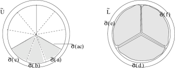
Figure 3: Chosen liftings for the simplices of Figure 2, when $n=3$.

So $U_{\sigma(a)}=U_{\sigma(b)}=U_{\sigma(c)}=\tilde{U}$, whereas $U_{\sigma(d)}=U_{\sigma(e)}=U_{\sigma(f)}=\tilde{L}$.

3.2 The $\mu$-maps.

Using these liftings we define the maps

$$\mu_{\sigma(ijk),\sigma(ij),\sigma(i),\sigma(j)}\colon G_{v(\sigma(ijk))}\rightarrow G_{v(\sigma(ij))}$$

for every pair $\sigma(i)$ and $\sigma(j)$ for which the intersection is a 1-simplex $\sigma(ij)$ and $\sigma(ijk)$ is a vertex with the same isotropy group as the interior of $\sigma(ij)$. Note that $G_{v(\sigma(ijk))}$ (where $\sigma(i)$, $\sigma(j)$ and $\sigma(k)$ are three different simplices) is trivial except for $G_{w}=G_{v(\sigma(abc))}=C_{n}$. So the only possibly non-trivial $\mu$-maps are those with codomain $G_{w}=G_{v(\sigma(ab))}=G_{v(\sigma(bc))}=G_{v(\sigma(ac))}$. In order to construct

$$\mu_{t,\sigma(ab),\sigma(a),\sigma(b)}\colon G_{t}\rightarrow G_{v(\sigma(ab))}=G_{w},$$

note that $\theta$, as used in Section 2.2, is $\sigma(a)\cap\sigma(b)$. We choose $W=U$ and $\tilde{\theta}=\tilde{\sigma}(a)\cap\tilde{\sigma}(b)$, so both $\gamma_{0}$ and $\gamma_{1}$, as used in Section 2.2, are the identity map. Moreover, we choose

$$\lambda_{\sigma(a),w}=\lambda_{\sigma(b),w}$$ (8)

(notation as in Section 2.1), whereas $\lambda_{\sigma(a),t}$ and $\lambda_{\sigma(b),t}$ have to be the same, because the liftings of $t$ in $\tilde{\sigma}(a)$ and $\tilde{\sigma}(b)$ are the same point in $\tilde{U}$. And it is obvious that

$$\mu_{t,\sigma(ab),\sigma(a),\sigma(b)}(1_{G_{t}})=1_{G_{v(\sigma(ab))}}.$$

Also (by the multiplicative property (3) of $\mu$),

$$\mu_{t,\sigma(ab),\sigma(b),\sigma(a)}(1_{G_{t}})=1_{G_{v(\sigma(ab))}}.$$

For similar reasons, when we choose

$$\lambda_{\sigma(b),w}=\lambda_{\sigma(c),w}$$ (9)

we find that both maps

$$\mu\colon G_{u}\rightarrow G_{v(\sigma(bc))}$$

are described by

$$\mu(1_{G_{u}})=1_{G_{v(\sigma(bc))}}.$$

The only non-trivial $\mu$-maps are $\mu_{v,\sigma(ac),\sigma(a),\sigma(c)}$, and $\mu_{v,\sigma(ac),\sigma(c),\sigma(a)}$ from $G_{v}$ into $G_{v(\sigma(ac))}=G_{w}$. With the notation of Section 2, $\theta=\sigma(ac)$ and we choose $W=U_{v}=U_{w}=U$ with $\tilde{\theta}=\tilde{\sigma}(ac)\subset\tilde{\sigma}(a)$ as in Figure 3. Moreover, we take

$$\lambda_{\sigma(a),w}=\lambda_{\sigma(a),v}=\gamma_{1}=\mbox{\rm id}.$$

Then (8) and (9) above induce that $\lambda_{\sigma(c),w}=\mbox{\rm id}.$ It follows from the choice of the liftings in Figure 3, that

$$\gamma_{0}=\lambda_{\sigma(c),v}=\rho,$$

where $\rho$ is rotation over $2(n-1)\pi/n$, which generates $G_{w}$. We conclude that the group elements $g_{0},g_{1},$ and $h_{1}$ are all the identity element, and $h_{0}=\rho$, so:

$$\mu_{v,\sigma(ac),\sigma(c),\sigma(a)}(1)=\rho.$$

Similarly one can show that:

$$\mu_{v,\sigma(ac),\sigma(a),\sigma(c)}(1)=\rho^{n-1}.$$

(This also follows from the fact that they have to be each other’s inverses by the multiplicative property of $\mu$ as stated in (3).)

3.3 The simplicial complex.

With these $\mu$-maps the simplicial complex can be described as follows.

$$S_{0} = \{\sigma(a),\sigma(b),\sigma(c),\sigma(d),\sigma(e),\sigma(f)\},$$

$$S_{n} = \{(\sigma(i_{0}\cdots i_{n}),g_{1},\cdots,g_{n});\,g_{1},\cdots,g_{n}\in G_{\sigma(i_{0}\cdots i_{n})}\mbox{ and }\sigma(i_{0}\cdots i_{n})\neq\emptyset\}.$$

The degeneracy maps $s_{i}$ are trivial as described in Section 2.1, and the face maps are straightforward compositions on all combinations which do not contain neighboring $a$ and $c$ in their $\sigma$-part, since the $\mu$-maps are trivial in these cases. For the $ac$-combinations, we have to use the non-trivial part of the $\mu$-maps described above. For example, deleting the sigma’s from the notation, we can describe the face operators on $S_{2}$ by:

$$d_{0}(f\stackrel{{\scriptstyle 1}}{{\longleftarrow}}c\stackrel{{\scriptstyle 1}}{{\longleftarrow}}a) = (c\stackrel{{\scriptstyle\rho}}{{\longleftarrow}}a),$$

$$d_{1}(f\stackrel{{\scriptstyle 1}}{{\longleftarrow}}c\stackrel{{\scriptstyle 1}}{{\longleftarrow}}a) = (f\stackrel{{\scriptstyle 1}}{{\longleftarrow}}a),$$

$$d_{2}(f\stackrel{{\scriptstyle 1}}{{\longleftarrow}}c\stackrel{{\scriptstyle 1}}{{\longleftarrow}}a) = (f\stackrel{{\scriptstyle 1}}{{\longleftarrow}}c).$$

So for $\alpha\in A_{\sigma(a)}$, we find that $(f\stackrel{{\scriptstyle 1}}{{\longleftarrow}}c)\cdot((c\stackrel{{\scriptstyle\rho}}{{\longleftarrow}}a)\cdot\alpha)=(f\stackrel{{\scriptstyle 1}}{{\longleftarrow}}a)\cdot\alpha$. We use this in the following calculation,

$$(a\stackrel{{\scriptstyle\,\rho}}{{\leftarrow}}a)\cdot\alpha = (a\stackrel{{\scriptstyle 1}}{{\leftarrow}}c)\cdot((c\stackrel{{\scriptstyle\,\rho}}{{\leftarrow}}a)\cdot\alpha)$$

$$= (a\stackrel{{\scriptstyle 1}}{{\leftarrow}}b)\cdot((b\stackrel{{\scriptstyle 1}}{{\leftarrow}}c)\cdot((c\stackrel{{\scriptstyle\,\rho}}{{\leftarrow}}a)\cdot\alpha))$$

$$= (a\stackrel{{\scriptstyle 1}}{{\leftarrow}}d)\cdot((d\stackrel{{\scriptstyle 1}}{{\leftarrow}}b)\cdot((b\stackrel{{\scriptstyle 1}}{{\leftarrow}}f)\cdot((f\stackrel{{\scriptstyle 1}}{{\leftarrow}}c)\cdot((c\stackrel{{\scriptstyle\,\rho}}{{\leftarrow}}a)\cdot\alpha))))$$

$$= (a\stackrel{{\scriptstyle 1}}{{\leftarrow}}f)\cdot((f\stackrel{{\scriptstyle 1}}{{\leftarrow}}d)\cdot((d\stackrel{{\scriptstyle 1}}{{\leftarrow}}e)\cdot((e\stackrel{{\scriptstyle 1}}{{\leftarrow}}b)\cdot((b\stackrel{{\scriptstyle 1}}{{\leftarrow}}f)\cdot$$

$$\cdot((f\stackrel{{\scriptstyle 1}}{{\leftarrow}}a)\cdot\alpha)))))$$

$$= (a\stackrel{{\scriptstyle 1}}{{\leftarrow}}f)\cdot((f\stackrel{{\scriptstyle 1}}{{\leftarrow}}e)\cdot((e\stackrel{{\scriptstyle 1}}{{\leftarrow}}f)\cdot((f\stackrel{{\scriptstyle 1}}{{\leftarrow}}a)\cdot\alpha)))$$

$$= (a\stackrel{{\scriptstyle 1}}{{\leftarrow}}f)\cdot((f\stackrel{{\scriptstyle 1}}{{\leftarrow}}a)\cdot\alpha)$$

$$= \alpha$$

(This calculation illustrates the effect of the fact that a loop around the singular point $v(\sigma(abc))$ is contractible via the lower half of the teardrop.)

3.4 The cohomology groups

We conclude from the above calculation that $C_{n}$ acts trivially on $A$, and it is not difficult to derive that:

$$H^{0}(\mbox{\it Tear-n};{\cal A})=A\mbox{ and }H^{1}(\mbox{\it Tear-n};{\cal A})=0.$$

To find the second cohomology group, we have to do some cocycle-coboundary calculations in the local system of coefficients $A$ on the simplicial set $S$. A cohomology class in $H^{2}$ is represented by a cocycle $\alpha\in Z^{2}(S,A)$, which we write as an $A$-valued map $\alpha\colon S_{2}\rightarrow A$. Since the second cohomology group of the plane is zero, we can choose the representant $\alpha$ in such a way that $\alpha(\sigma(ijk),g_{1},g_{2})=0$ when $\{i,j,k\}\cap\{d,e,f\}\neq\emptyset$ and moreover,
$\alpha(\sigma(aca),\rho^{n-1},\rho)=0$, $\alpha(\sigma(cac),\rho,\rho^{n-1})=0$, $\alpha(\sigma(aba),1,1)=0$, $\alpha(\sigma(bab),1,1)=0$, $\alpha(\sigma(bcb),1,1)=0$, $\alpha(\sigma(cbc),1,1)=0$.
It follows then from the cocycle-relations, that $\alpha$ is determined by the following data

$$\left\{\begin{array}[]{lll}\alpha(\sigma(caa),1,\rho^{i})&\alpha(\sigma(bba),\rho^{i},1)&\alpha(\sigma(cbb),1,\rho^{i})\\ &\alpha(\sigma(aab),\rho^{i},1)&\alpha(\sigma(ccb),\rho^{i},1)\\ \alpha(\sigma(acc),1,\rho^{i})&\alpha(\sigma(baa),1,\rho^{i})&\alpha(\sigma(bbc),\rho^{i},1)\\ \alpha(\sigma(aaa),\rho^{i},\rho^{j})&\alpha(\sigma(abc),1,1)&\end{array}\right.\mbox{ for }i,j\in\{1,2,\cdots,n-1\}.$$ (10)

By choosing an appropriate coboundary, one can find an equivalent cocycle $\alpha^{\prime}$, such that of all the values in (10) above, only $\alpha^{\prime}(\sigma(abc),1,1)$ need not be zero. Moreover, two cocycles $\alpha_{1}$ and $\alpha_{2}$ of this form are equivalent iff $\alpha_{1}(\sigma(abc),1,1)=\alpha_{2}(\sigma(abc),1,1)$. We conclude:

$$H^{2}(\mbox{\it Tear-n};{\cal A})=A.$$

The higher degree cohomology groups of Tear-n can be calculated using the Mayer-Vietoris sequence for the upper and lower half-sphere, denoted by $U_{n}$ and $L$, for $m>2$:

We conclude:

Theorem 3.4.1

The teardrop orbifold Tear-n has the following cohomology groups:

$$H^{0}(\mbox{{\it Tear-n}};{\cal A}) = A;$$

$$H^{1}(\mbox{{\it Tear-n}};{\cal A}) = 0;$$

$$H^{2}(\mbox{{\it Tear-n}};{\cal A}) = A;$$

$$H^{m}(\mbox{{\it Tear-n}};{\cal A}) = H^{m}(C_{n};A),\mbox{ for }m>2.$$

4 Topological groupoids for orbifolds.

Again, we fix an orbifold ${\cal M}$ with underlying space $M$ and atlas ${\cal U}$. Recall from Section 1.3 the category ${\it Ab}({\cal M})$ of all abelian sheaves on ${\cal M}$. In [7, Theorem 4.1] we proved that this category can be represented as the category of equivariant sheaves in various ways. Here we single out one particular such representation.

4.1 Etale groupoids.

Let $G$ be a topological groupoid. As in loc. cit., we write $G_{0}$ for the space of objects and $G_{1}$ for the space of arrows, while the structure maps are denoted:

for composition, source, target, units and inverse, respectively. As usual, we write $1_{x}$ for $u(x)$, $g^{-1}$ for $i(g)$, $g\circ h$ or $gh$ for $m(g,h)$, and $g\colon x\rightarrow y$ if $s(g)=x$ and $t(g)=y$. The groupoid $G$ is said to be étale if $s$ and $t$ are local homeomorphisms, and proper if $(s,t)\colon G_{1}\rightarrow G_{0}\times G_{0}$ is a proper map.

A $G$-sheaf is a sheaf $A$ on the space $G_{0}$, equipped with a continuous (say, right) action by $G_{1}$. The category of all $G$-sheaves is denoted ${\it Ab}(G)$. We recall from [7]:

Theorem 4.1.1

For any orbifold ${\cal M}$ there exists a proper and étale topological groupoid $G$, for which there is a natural equivalence ${\it Ab}({\cal M})\cong{\it Ab}(G)$.

One construction of $G$ from ${\cal M}$, suggested in [5] and different from that in [7], is the following. Let $G_{0}$ be the space of pairs $(\tilde{x},\tilde{U})$ with $\tilde{x}\in\tilde{U}\in{\cal U}$, topologized as the disjoint sum of the sets $\tilde{U}$ in ${\cal U}$. An arrow $g\colon(\tilde{x},\tilde{U})\rightarrow(\tilde{y},\tilde{V})$ is an equivalence class of triples

$$g=[\lambda,\tilde{z},\mu]\colon\,\tilde{U}\stackrel{{\scriptstyle\lambda}}{{\longleftarrow}}\tilde{W}\stackrel{{\scriptstyle\mu}}{{\longrightarrow}}\tilde{V},$$

where $\tilde{z}\in\tilde{W}$ and $\lambda(\tilde{z})=\tilde{x}$, $\mu(\tilde{z})=\tilde{y}$. Here $\tilde{W}$ is another chart for ${\cal M}$, and $\lambda,\,\mu$ are embeddings. The equivalence relation is generated by

$$[\lambda,\tilde{z},\mu]=[\lambda\nu,\tilde{z}^{\prime},\mu\nu],$$

for $\lambda,\,\tilde{z},\,\mu$ above and $\nu\colon\tilde{W}^{\prime}\rightarrow\tilde{W}$ another embedding, with $\nu(\tilde{z}^{\prime})=\tilde{z}$. There is a natural topology on the set $G_{1}$ of all these equivalence classes, for which the source and target maps $s,t\colon G_{1}\rightarrow G_{0}$ are each étale and together give a proper map $G_{1}\rightarrow G_{0}\times G_{0}$. (See [8] for details.) Note that one can take any chart, not necessarily from the chosen atlas ${\cal U}$, to represent an arrow, as it will always be equivalent to one represented by a chart in ${\cal U}$. (In fact, given a chart $\tilde{W}$ around $\varphi(\tilde{x})$ which is embeddable into $\tilde{U}$ and $\tilde{V}$, every arrow $g\colon(\tilde{x},\tilde{U})\rightarrow(\tilde{y},\tilde{V})$ can be represented by a triple involving $\tilde{W}$.)

For $G$ constructed in this way, it is not difficult to see that there is an equivalence of categories ${\it Ab}({\cal M})\simeq{\it Ab}(G)$.

If $G$ is any topological groupoid, its nerve $\mbox{Nerve}(G)$ is the simplicial space whose $n$-simplices are strings $\stackrel{{\scriptstyle\rightarrow}}{{g}}=(x_{0}\stackrel{{\scriptstyle g_{1}}}{{\leftarrow}}\cdots\stackrel{{\scriptstyle g_{n}}}{{\leftarrow}}x_{n})$, equipped with the natural (fibered product) topology. One writes $G_{n}$ for the space $\mbox{Nerve}(G)_{n}$ of these $n$-simplices. If $A$ is any $G$-sheaf, it induces a sheaf $A^{(n)}$ on $G_{n}$, with stalk $A^{(n)}_{\stackrel{{\scriptstyle\rightarrow}}{{g}}}=A_{x_{n}}$.

Proposition 4.1.2

Let $G$ be any étale topological groupoid representing the orbifold ${\cal M}$ as in Theorem 4.1.1. For each abelian sheaf ${\cal A}$ on ${\cal M}$, there is a natural spectral sequence

$$E^{p,q}_{2}=H^{p}H^{q}(G_{\bullet},A^{(\bullet)})\Rightarrow H^{p+q}({\cal M},{\cal A}).$$

(Here ${\cal A}$ corresponds by Theorem 4.1.1 to a $G$-sheaf $A$, with induced sheaf $A^{(p)}$ on $G_{p}$, so that for fixed $q$, $H^{q}(G_{\bullet},A^{(\bullet)})$ is a cosimplicial group.)

Proof.

Using the equivalence of Theorem 4.1.1, this spectral sequence is simply a special case of the standard one,

$$H^{p}H^{q}(G_{\bullet},A^{\bullet})\Rightarrow H^{p+q}(G,A),$$

for étale topological groupoids (see [1, V, (7.4.0.3)]). For later use, we recall that the latter spectral sequence is constructed from the double complex $\Gamma(G_{p},I^{q(p)})$, where $A\rightarrow I^{0}\rightarrow I^{1}\rightarrow\cdots$ is any injective resolution in ${\it Ab}(G)$. This induces a resolution $A^{(p)}\rightarrow I^{0(p)}\rightarrow I^{1(p)}\rightarrow I^{2(p)}\rightarrow\cdots$ of sheaves on $G_{p}$ which is again injective.

4.2 Proper groupoids.

The groupoid $G$ for ${\cal M}$ in Theorem 4.1.1 is not unique. (However, it is unique up to weak, or ‘Morita’ equivalence [7].) For the proof of Theorem 2.1.1, we will use the following construction. Let $H_{0}\hookrightarrow G_{0}$ be a closed subspace. Then $H_{0}$ is the space of objects of a topological groupoid $H$, with $H_{1}$ constructed as the fibered product

(11)

In other words, $H$ is the full subgroupoid of $G$ on the space of objects $H_{0}\subseteq G_{0}$. (This topological groupoid $H$ is in general not étale.)

Lemma 4.2.1

Assume the closed subspace $H_{0}\subseteq G_{0}$ has the property that the map:

$$s\circ\pi_{2}\colon H_{0}\times_{G_{0}}G_{1}\rightarrow G_{0},\quad(x\in H_{0},(g\colon y\rightarrow x)\in G_{1})\mapsto y$$

is a proper surjection. Then the inclusion of groupoids $H\subseteq G$ induces an equivalence of categories ${\it Ab}(H)\simeq{\it Ab}(G)$.

Proof.

Standard. (See [8] for details.)

Corollary 4.2.2

Let ${\cal M}$ be an orbifold, let $G$ be an étale groupoid representing ${\cal M}$ as in Theorem 4.1.1, and let $H\subseteq G$ be any subgroupoid as constructed above. Then there exists a natural spectral sequence

$$E^{p,q}_{2}=H^{p}H^{q}(H_{\bullet},A^{(\bullet)}|H_{\bullet})\Rightarrow H^{p+q}({\cal M,A}).$$

(Here $H_{p}\subseteq G_{p}=\mbox{Nerve}(G)_{p}$ and $A^{(p)}|H_{p}$ is the restricted sheaf.)

Proof.

This is proved in the same way as in Proposition 4.1.2, using that the injective sheaves $I^{(q)p}$ on $G_{p}$ restrict to soft sheaves on the closed subspace $H_{p}\subseteq G_{p}$.

4.3 Proof of Theorem 2.1.1.

Our purpose in this section is to construct a specific subgroupoid $H\subset G$ for ${\cal M}$ from a given triangulation. First, observe the following method for constructing a groupoid $H\subseteq G$ as in Lemma 4.2.1. Let ${\cal F}=\{F_{i}\}_{i\in I}$ be a locally finite cover of $M$ by compact sets, which refines the cover of charts, say $F_{i}\subset U_{i}$. Suppose there are chosen liftings $\tilde{F}_{i}\subset\tilde{U}_{i}$, where the quotient map $\varphi_{i}\colon\tilde{U}_{i}\rightarrow U_{i}$ of the chart maps $\tilde{F}_{i}$ homeomorphically to $F_{i}$. Let $H_{0}=\{(x,\tilde{F}_{i})|x\in\tilde{F}_{i},i\in I\}$ be the disjoint sum of these sets $\tilde{F}_{i}$. Then $H_{0}$ is a closed subset of $G_{0}$. The induced groupoid $H$, with $H_{1}$ constructed as the fibered product in (11), is denoted $H({\cal F})$.

Lemma 4.3.1

For any locally finite cover ${\cal F}$ as above, the map $s\pi_{2}\colon H_{0}\times_{G_{0}}G_{1}\rightarrow G_{0}$ is a proper surjection, and hence the inclusion $H({\cal F})\subseteq G$ induces an equivalence ${\it Ab}(H)\simeq{\it Ab}(G)\simeq{\it Ab}({\cal M})$.

Proof.

The second statement follows from the first by Lemma 4.2.1. It follows immediately from the fact that the $F_{i}$ cover $M$ that $s\pi_{2}\colon H_{0}\times_{G_{0}}G_{1}\rightarrow G_{0}$ is a surjection. To check that $s\pi_{2}$ is also proper, it suffices to prove that each point in $G_{0}$ has a neighborhood $\tilde{V}$ over which $s\pi_{2}$ is a proper map $s\pi_{2}^{-1}(\tilde{V})\rightarrow\tilde{V}$. Choose $(\tilde{x},\tilde{U}_{j})\in G_{0}$ and let $\tilde{V}\subseteq\tilde{U}_{j}$ be a neighborhood of $\tilde{x}$ such that $V=\varphi_{j}(\tilde{V})\subseteq M$ meets only finitely many $F_{i}$, say $F_{i_{1}},\cdots,F_{i_{n}}$. Then $s\pi_{2}^{-1}(\tilde{V})=\sum_{k=1}^{n}\tilde{F}_{i_{k}}\times_{G_{0}}G_{1}\times_{G_{0}}\tilde{V}$, and it suffices to show that each $\tilde{F}_{i_{k}}\times_{G_{0}}G_{1}\times_{G_{0}}\tilde{V}\rightarrow\tilde{V}$ is proper. Now $(s,t)\colon G_{1}\rightarrow G_{0}\times G_{0}$ is proper (Theorem 4.1.1), hence so is its pullback $(\pi_{1},\pi_{3})\colon\tilde{F}_{i_{k}}\times_{G_{0}}G_{1}\times_{G_{0}}\tilde{V}\rightarrow F_{i_{k}}\times\tilde{V}$. Since $\tilde{F}_{i_{k}}$ is compact, the map $\tilde{F}_{i_{k}}\times_{G_{0}}G_{1}\times_{G_{0}}\tilde{V}\rightarrow\tilde{V}$ is also proper, as required.

Now fix a triangulation ${\cal T}$ adapted to ${\cal U}$, so the conditions (i) and (ii) from the beginning of Section 2.1 are satisfied. Consider the locally finite cover of $M$ by simplices $\sigma\in{\cal T}$ of maximal dimension $n$. Fix for each $\sigma$ a chart $U_{\sigma}\supseteq\sigma$ and a lifting $\tilde{\sigma}\subseteq\tilde{U}_{\sigma}$ as before. Let $H({\cal T})\subseteq G$ be the full subgroupoid constructed from this cover. Thus $H({\cal T})_{0}$ is the disjoint sum of the $n$-simplices in ${\cal T}$, and $H({\cal T})_{1}$ is constructed as the pullback. By Lemma 4.3.1, the inclusion $H({\cal T})\subseteq G$ induces an equivalence of categories of sheaves.

We will show (cf. Proposition 4.3.3 below), that the space $H({\cal T})_{1}$ is also a disjoint sum of simplices. To be able to do that, we need a canonical way of representing the arrows. We will use a refining atlas and a subdivision of the triangulation ${\cal T}$ to achieve this. Let ${\cal V}\succcurlyeq{\cal U}$ be a good atlas refining ${\cal U}$, and let ${\cal T}^{\prime}$ be a subdivision of ${\cal T}$ which is good for ${\cal V}$ (cf. Section 1.2). Thus, each simplex $\tau\in{\cal T}^{\prime}$ is contained in a contractible chart $V_{\tau}$ in ${\cal V}$. Furthermore, since ${\cal V}$ is a good atlas, these charts $V_{\tau}$ can be chosen in such a way, that $V_{\tau^{\prime}}\subseteq V_{\tau}$ whenever $\tau^{\prime}\subseteq\tau$. Moreover, we may assume $V_{\tau}\subseteq U_{\sigma}$ whenever the simplex $\tau\in{\cal T}^{\prime}$ is contained in the $n$-simplex $\sigma\in{\cal T}$. For each $\tau\in{\cal T}^{\prime}$, choose one $n$-simplex $\sigma\in{\cal T}$ containing $\tau$ and an embedding $\lambda_{\sigma,\tau}\colon\tilde{V}_{\tau}\rightarrow\tilde{U}_{\sigma}$ with the lifting of $\tau$ in $\tilde{\sigma}$ in its image. Then let $\tilde{\tau}=\lambda_{\sigma,\tau}^{-1}(\tau\subseteq\tilde{\sigma})$, be the lifting of $\tau$ in $\tilde{V}_{\tau}$. Next, for every other $n$-simplex $\sigma\in{\cal T}$ containing $\tau$, choose an embedding

$$\lambda_{\sigma,\tau}\colon\tilde{V}_{\tau}\rightarrow\tilde{U}_{\sigma}\mbox{ with }\lambda_{\sigma,\tau}(\tilde{\tau})\subseteq\tilde{\sigma}.$$ (12)

We need some explicit notation for these charts, and denote them by

$$(\tilde{U}_{\sigma},G_{\sigma},\varphi_{\sigma}\colon\tilde{U}_{\sigma}\rightarrow U_{\sigma})\mbox{ and }(\tilde{V}_{\tau},H_{\tau},\psi_{\tau}\colon\tilde{V}_{\tau}\rightarrow V_{\tau}).$$

Furthermore, we denote by $H_{\mathord{\mathop{\tau}\limits^{\smash{\circ}}}}\subseteq H_{\tau}$ the isotropy group of the interior of $\tau$ (or of $\tilde{\tau}$).

Note that the space of arrows $H({\cal T})_{1}$ is the disjoint sum of spaces

$$H({\cal T})(\sigma_{0},\sigma_{1})=\{g\in G_{1}|\,s(g)\in\tilde{\sigma}_{1}\subseteq\tilde{U}_{\sigma_{1}}\mbox{ and }t(g)\in\tilde{\sigma}_{0}\subseteq\tilde{U}_{\sigma_{0}}\}$$

of arrows from $\tilde{\sigma}_{1}$ to $\tilde{\sigma}_{0}$. Consider one of these spaces.

By assumption on the triangulation ${\cal T}$, there is a family of faces of $\rho=\sigma_{0}\cap\sigma_{1}$,

$$\rho=\rho_{k}\supseteq\rho_{k-1}\supseteq\cdots\supseteq\rho_{0},$$ (13)

such that the isotropy is constant on $\rho_{i}-\rho_{i-1}$. We may assume that $\rho_{0}=v(\rho)$ is the chosen vertex with maximal isotropy. By working with the liftings $\tilde{\sigma}_{i}\,(i=0,1)$ and the associated liftings $\tilde{\rho}^{i}=\tilde{\rho}_{k}^{i}\supseteq\tilde{\rho}_{k-1}^{i}\supseteq\cdots\supseteq\tilde{\rho}_{0}^{i}$ contained in $\tilde{\sigma}_{i}$, the isotropy subgroups form an increasing family of subgroups of the groups $G_{\sigma_{i}}$,

$$G_{k}^{i}\subseteq G_{k-1}^{i}\subseteq\cdots\subseteq G_{0}^{i}\subseteq G_{\sigma_{i}},$$ (14)

where $G_{0}^{i}=G_{v(\rho^{i})}$ is the isotropy group of the lifted vertex $\tilde{\rho}^{i}_{0}$ of $\tilde{\sigma}_{i}$. The filtration (13) yields a similar filtration of the space of arrows $H({\cal T})(\sigma_{0},\sigma_{1})$. To see this, consider any arrow $g\colon\tilde{x}_{1}\rightarrow\tilde{x}_{0}$ in $H({\cal T})(\sigma_{0},\sigma_{1})$. Then in the underlying space $M$ we have $x_{0}=x_{1}\in\rho$, so $x_{0}=x_{1}$ is contained in one of the simplices $\tau$ of ${\cal T}^{\prime}$. It follows that every arrow can be represented in the form

$$\tilde{U}_{\sigma_{0}}\stackrel{{\scriptstyle\lambda_{0}}}{{\longleftarrow}}\tilde{V}_{\tau}\stackrel{{\scriptstyle\lambda_{1}}}{{\longrightarrow}}\tilde{U}_{\sigma_{1}}\quad g=[\lambda_{0}\circ\ell,\tilde{z},\lambda_{1}]$$ (15)

where $\lambda_{i}=\lambda_{\sigma_{i},\tau}\,\,(i=0,1)$ are the chosen embeddings in (12), $\tilde{z}\in\tilde{\tau}\subseteq\tilde{V}_{\tau}$ is the unique point with $\lambda_{i}(\tilde{z})=\tilde{x}_{i}$, and $l\in H_{\tilde{z}}\subseteq H_{\tau}$ fixes the interior of $\tilde{\tau}$, i.e. $l\in H_{\mathord{\mathop{\tau}\limits^{\smash{\circ}}}}$. Let us say that an arrow $g$ represented as in (15) has rank $\geq k$ if $l\in H_{\mathord{\mathop{\tau}\limits^{\smash{\circ}}}}$ where $\tau\subseteq\rho_{k}$.

For an arrow of rank at least $k$, the following lemma gives a criterion as to whether the rank is strictly larger than $k$.

Lemma 4.3.2

Consider the open sets

$$\tilde{N}_{i}=\lambda_{i}^{-1}(\tilde{\rho}_{k+1}^{i}-\tilde{\rho}_{k}^{i})\qquad(i=0,1)$$

where $\tilde{\rho}_{k+1}^{i},\tilde{\rho}_{k}^{i}\subseteq\tilde{\sigma}_{i}$. An arrow $g$ as in (15) of rank $\geq k$ is of rank $\geq k+1$ if and only if there is an open neighborhood $W_{\tau}$ of $\tilde{\tau}$ in $\tilde{N}_{1}\cup\tilde{\tau}$ such that for every $\tilde{y}_{1}\in(W_{\tau}-\tau)$, the image $\tilde{y}_{0}=\ell\cdot\tilde{y}_{1}$ belongs to $\tilde{N}_{0}$.

Proof.

Suppose that $g$ as represented in (15) has rank $\geq k+1$. Let $\tau^{\prime}\supseteq\tau$ be any simplex in ${\cal T}^{\prime}$ with $\tau^{\prime}\subseteq\rho_{k+1}$, and consider the following diagram

(16)

where $\lambda_{i}=\lambda_{\sigma_{i},\tau}$ as above and $\overline{\lambda}_{i}=\lambda_{\sigma_{i},\tau^{\prime}}$, while $\nu$ is any embedding mapping the chosen lifting $\tilde{\tau}\subseteq\tilde{V}_{\tau}$ into $\tilde{\tau}^{\prime}$. Furthermore, $a_{0},a_{1}\in H_{\tau}$ are group elements such that

$$\lambda_{i}\circ a_{i}=\overline{\lambda}_{i}\circ\nu.$$ (17)

Then by the equivalence relation defining $G_{1}$, the arrow $g=[\lambda_{0}\circ\ell,\tilde{z},\lambda_{1}]$ can be represented as

$$g=[\overline{\lambda}_{0}\circ\ell^{\prime},\nu(\tilde{z}),\overline{\lambda}_{1}]\quad\ell^{\prime}=\nu(a_{0}^{-1}\ell a_{1}),$$ (18)

and $\ell^{\prime}\in H_{\mathord{\mathop{\tau}\limits^{\smash{\circ}}\negthinspace{}^{\prime}}}$ by assumption. Let $y\in(\tau^{\prime}-\tau)\cap U_{\sigma_{0}}\cap U_{\sigma_{1}}\cap V_{\tau}\subseteq(\rho_{k+1}-\rho_{k})$ be any point, and denote its liftings in $\tilde{\sigma}_{i}\,(i=0,1)$ by $y_{i}$. Let $\tilde{y}_{i}=\lambda_{i}^{-1}(y_{i})\in\tilde{N}_{i}\subset\tilde{V}_{\tau}$. We claim that

$$\ell\cdot\tilde{y}_{1}=\tilde{y}_{0}\;.$$

Indeed, $\bar{\lambda}_{i}\nu(a^{-1}_{i}\tilde{y}_{i})=\lambda_{i}(\tilde{y}_{i})\in\tilde{\sigma}_{i}$, and hence $\nu(a^{-1}_{i}\;\tilde{y}_{i})\in\tilde{\tau}^{\prime}$ because $\bar{\lambda}_{i}$ is chosen to map $\tilde{\tau}^{\prime}$ into $\tilde{\sigma}_{i}$. It then follows first that $\nu(a^{-1}_{0}\;\tilde{y}_{0})=\nu(a^{-1}_{1}\;\tilde{y}_{1})$, since both sides are liftings in $\tilde{\tau}^{\prime}$ of the same point $y$, and next that this point in $\tilde{\tau}^{\prime}$ is fixed by $\ell^{\prime}$ since $\ell^{\prime}\in H_{\mathord{\mathop{\tau}\limits^{\smash{\circ}}\negthinspace{}^{\prime}}}$. Thus $\ell^{\prime}\cdot\nu(a^{-1}_{1}\tilde{y}_{1})=\nu(a^{-1}_{0}\tilde{y}_{0})$; or, by definition of $\ell^{\prime}$ in (15) above, $\nu(a^{-1}_{0}\ell\tilde{y}_{1})=\nu(a^{-1}_{0}\tilde{y}_{0})$. Since $\nu$ is an embedding, we conclude that $\ell\tilde{y}_{1}=\tilde{y}_{0}$, as claimed. So for every $\tau^{\prime}\supseteq\tau$ with $\tau^{\prime}\subseteq\rho_{k+1}$ and every $y\in(\tau^{\prime}-\tau)\cap\varphi_{\tau}(\tilde{N}_{0})\cap\varphi_{\tau}(\tilde{N}_{1})$ with liftings $\tilde{y}_{i}\in\tilde{N}_{i}$, we find that $\ell\cdot\tilde{y}_{1}=\tilde{y}_{0}$. Therefore

$$\varphi_{\tau}^{-1}\left\{\coprod_{\tau\subseteq\tau^{\prime}\subseteq\rho_{k+1}}(\tau^{\prime}\cap\varphi_{\tau}(\tilde{N}_{0}))\right\}\cap\tilde{N}_{1}$$

satisfies the requirements for $W_{\tau}$. So we have shown that $g$ satisfies the condition formulated in this lemma.

Now assume that the arrow $g$ is of rank $\geq k$ and satisfies this condition. Let $\tau^{\prime}\supseteq\tau$ be a simplex in $\rho_{k+1}$. Then its inverse image in $\tilde{N}_{1}$ has a nonempty intersection with $W_{\tau}$, so its inverse images in $\tilde{N}_{i}$ contain points $\tilde{y}_{i}$ as in the lemma. Use diagram (16) again to label all the embeddings and group elements involved. Then $g$ can again be represented as in (18) and we need to show that $\ell^{\prime}$ in that presentation is an element of $H_{\mathord{\mathop{\tau}\limits^{\smash{\circ}}\negthinspace{}^{\prime}}}$. Let $\tilde{y}_{0}$ and $\tilde{y}_{1}$ be as in the lemma, such that $\tilde{y}_{i}\in\psi_{\tau}^{-1}(\mathord{\mathop{\tau}\limits^{\smash{\circ}}\negthinspace{}^{\prime}})$. Then $\ell\cdot\tilde{y}_{1}=\tilde{y}_{0}$, so $\nu(\ell a_{1})\cdot(\overline{\lambda}_{1}^{\,-1}(\lambda_{1}(\tilde{y}_{1})))=\nu(a_{0}^{-1})\cdot(\overline{\lambda}_{0}^{\,-1}(\lambda_{0}(\tilde{y}_{0})))\in\tilde{V}_{\tau^{\prime}}$, or $\nu(a_{0}^{-1}\ell a_{1})\cdot(\overline{\lambda}_{1}^{\,-1}(\lambda_{1}(\tilde{y}_{1})))=\overline{\lambda}_{0}^{\,-1}(\lambda_{0}(\tilde{y}_{0}))$. However, both $\overline{\lambda}_{1}^{\,-1}(\lambda_{1}(\tilde{y}_{1}))$ and $\overline{\lambda}_{0}^{\,-1}(\lambda_{0}(\tilde{y}_{0}))$ are liftings in $\tilde{\tau}^{\prime}$ of the same point in $M$, so they have to be the same in $\tilde{\tau}^{\prime}$ as well. We conclude that $\ell^{\prime}=\nu(a_{0}^{-1}\ell a_{1})\in H_{\overline{\lambda}_{1}^{\,-1}(\lambda_{1}(\tilde{y}_{1}))}=H_{\mathord{\mathop{\tau}\limits^{\smash{\circ}}\negthinspace{}^{\prime}}}$ (since the isotropy is constant on the interior of a simplex) as required.

Now we are ready to prove:

Proposition 4.3.3

The space $H({\cal T})_{1}$ is (homeomorphic to) a disjoint sum of simplices.

Proof.

Let $\sigma_{0}$ and $\sigma_{1}$ be $n$-simplices in ${\cal T}$ and suppose that $\sigma_{0}\cap\sigma_{1}\neq\emptyset$. As we remarked before, it is sufficient to prove that $H({\cal T})(\sigma_{0},\sigma_{1})$ consists of a disjoint sum of simplices. Let $\rho_{j}$ be a part of the filtration (13) above. Write

$$\rho_{j}=\tau_{1}\cup\cdots\cup\tau_{m},$$ (19)

where $\tau_{i}$ are simplices in ${\cal T}^{\prime}$ of the same dimension as $\rho_{j}$. Consider all arrows of the form (15),

$$\tilde{U}_{\sigma_{0}}\stackrel{{\scriptstyle\lambda_{0,i}}}{{\longleftarrow}}\tilde{V}_{\tau_{i}}\stackrel{{\scriptstyle\lambda_{1,i}}}{{\longrightarrow}}\tilde{U}_{\sigma_{1}}\quad g=[\lambda_{0,i}\circ l,\tilde{z},\lambda_{1,i}]$$

where $\lambda_{\varepsilon,i}=\lambda_{\sigma_{\varepsilon},\tau_{i}}$ $\varepsilon=0,1;\,(i=1,\cdots,m)$ are the chosen embeddings as in (12), and $g$ has rank exactly $j$. For fixed $i$ and $\ell$, these arrows form a copy $\tau_{i}(\ell)$ of the simplex $\tau_{i}$. Moreover, if $\theta=\tau_{i}\cap\tau_{i^{\prime}}$ is a nonempty face not in the boundary of $\rho_{j}$ then this copy $\tau_{i}(\ell)$ is glued (along $\theta$) to exactly one copy $\tau_{i^{\prime}}(\ell^{\prime})$ in the space $H({\cal T})(\sigma_{0},\sigma_{1})$, as follows.

Since ${\cal T}^{\prime}$ is a good triangulation, there are embeddings $\nu\colon\tilde{V}_{\theta}\rightarrow\tilde{V}_{\tau_{i}}$ and $\nu^{\prime}\colon\tilde{V}_{\theta}\rightarrow\tilde{V}_{\tau_{i^{\prime}}}$, mapping $\tilde{\theta}$ to $\tilde{\tau}_{i}$ and $\tilde{\tau}_{i^{\prime}}$, respectively. Thus there are $a_{0},a_{1},b_{0},b_{1}\in H_{\theta}$ such that

$$\lambda_{\sigma_{j},\theta}a_{j} = \lambda_{j,i}\nu\quad(j=0,1)$$

$$\lambda_{\sigma_{j},\theta}b_{j} = \lambda_{j,i^{\prime}}\nu^{\prime}$$

Let $\ell^{\prime}$ and $\ell^{\prime\prime}$ be such that $\ell=\nu(\ell^{\prime\prime})$ and $\ell^{\prime}=\nu^{\prime}(b_{0}^{-1}a_{0}\ell^{\prime\prime}a_{1}^{-1}b_{1})$. Then $\tau_{i}(\ell)$ is glued to $\tau_{i^{\prime}}(\ell^{\prime})$. (Notice that $g=[\lambda_{0,i}\circ\ell,\tilde{z},\lambda_{1,i}]$ has rank exactly $j$ if and only if $g^{\prime}=[\lambda_{0,i^{\prime}}\circ\ell^{\prime},\tilde{z}^{\prime},\lambda_{1,i^{\prime}}]$ does. This follows from Lemma 4.3.2, since every pair of open neighborhoods of $\tau_{i}$ and $\tau_{i^{\prime}}$ have a non-empty intersection. )

Thus, the subspace of all $H({\cal T})(\sigma_{0},\sigma_{1})$ of all these copies $\tau_{i}(\ell)$ is a covering projection of $\rho_{j}$, hence a disjoint sum of copies of $\rho_{j}$.

Finally every arrow $g\in H({\cal T})(\sigma_{0},\sigma_{1})$ occurs in this way, i.e. is represented in the form (15) where $\tau_{i}\subseteq\rho_{j}$ is one of the simplices in (19) and $g$ has rank exactly $j$. (This follows easily from considerations as in the proof of Lemma 4.3.2.)

Lemma 4.3.4

Each space $H({\cal T})_{n}$ in the nerve of the groupoid $H({\cal T})$ is a disjoint sum of simplices.

Proof

This is clear from the fact that $H({\cal T})_{0}$ and $H({\cal T})_{1}$ are sums of simplices, while $H({\cal T})_{n}$ is constructed as an iterated fibered product along the source and target maps, which are embeddings on every component of $H({\cal T})_{1}$.

Now consider the spectral sequence of Corollary 4.2.2. Let ${\cal A}$ be any locally constant sheaf on ${\cal M}$, and let $A$ be the associated $H$-sheaf. Each sheaf $A^{(p)}$ on $H_{p}$ is again locally constant, hence constant on each connected component. So in fact $A^{(\bullet)}$ corresponds to a local system of coefficients on the simplicial set $\pi_{0}(H({\cal T})_{\bullet})$, obtained by taking the connected components of the space $H({\cal T})_{n}$ in the nerve. Since each such connected component is a simplex, the spectral sequence of Corollary 4.2.2 collapses, to give the following isomorphism.

Lemma 4.3.5

For any locally constant sheaf ${\cal A}$ on ${\cal M}$ there is a natural isomorphism

$$H^{p}(\pi_{0}(H({\cal T})_{\bullet}),A)=H^{p}({\cal M,A}),$$

where $A$ is the local system of coefficients on the simplicial set $\pi_{0}(H({\cal T})_{\bullet})$ induced by ${\cal A}$.

The proof of Theorem 2.1.1 is now completed by the observation that this simplicial set is exactly the simplicial set $S$ described in Section 2.

Lemma 4.3.6

There is a natural isomorphism of simplicial sets

$$\pi_{0}(H({\cal T})_{\bullet})\stackrel{{\scriptstyle\sim}}{{\longrightarrow}}S.$$

Proof.

By definition, $\pi_{0}(H({\cal T})_{0})=S_{0}$ in case $n=0$. For $n>0$ the identity follows from the fact that the definition of $\mu$ is related to the equivalence relation on $H({\cal T})_{1}\subseteq G_{1}$ in the following way. Let $\sigma_{0}$ and $\sigma_{1}$ be $n$-simplices as before and let $v$ and $w$ be vertices in $\sigma_{0}\cap\sigma_{1}$, connected by a 1-simplex $\theta$ and suppose that $w=v(\theta)$. Then $[\lambda_{\sigma_{0},v}\circ g,\tilde{v},\lambda_{\sigma_{1},v}]$ and $[\lambda_{\sigma_{0},w}\circ h,\tilde{w},\lambda_{\sigma_{1},w}]$ are in the same connected component of $H({\cal T})_{1}$ if an only if $h=\mu(g)$.

As said, this completes the proof of Theorem 2.1.1.

I. Moerdijk	D.A. Pronk
Mathematical Institute	Department of Mathematics
Utrecht University	Dalhousie University
PO Box 80010	Halifax, NS
3508 TA, Utrecht	Canada, B3H 3J5
The Netherlands
moerdijk@math.ruu.nl	pronk@cs.dal.ca

References

- [1] M.Artin, A. Grothendieck, J.L. Verdier, Théorie des Topos et Cohomologie Etale des Schémas, SGA4, tome 2, L.N.M. 270, Springer-Verlag, New York, 1972.
- [2] R. Bott, L.W. Tu, Differential Forms in Algebraic Topology, Springer-Verlag, New York, 1982.
- [3] M.W. Davis, J.W. Morgan, Finite group actions on homotopy 3-spheres, in The Smith Conjecture, Academic Press, 1984, pp. 181-226.
- [4] R.M. Goresky, Triangulation of stratified objects, Proc. of the A.M.S. 72 (1978), pp.193-200.
- [5] A. Haefliger, Groupoïdes d’holonomie et classifiants, Astérisque 116 (1984), pp.70-97.
- [6] J.L. Koszul, Sur certains groupes de transformations de Lie. Géometrie différentielle. Colloq. Int. Cent. Nat. Rech. Sci. Strasbourg (1953), pp. 137-141.
- [7] I. Moerdijk, D.A. Pronk, Orbifolds, sheaves and groupoids, to appear in K-theory.
- [8] D.A. Pronk, Groupoid Representations for Sheaves on Orbifolds, Ph.D. thesis, Utrecht 1995.
- [9] I. Satake, On a generalization of the notion of manifold, Proc. of the Nat. Acad. of Sc. U.S.A. 42 (1956), pp. 359-363.
- [10] I. Satake, The Gauss-Bonnet theorem for V-manifolds, Journal of the Math. Soc. of Japan 9 (1957), pp. 464-492.
- [11] W.P. Thurston, Three-Dimensional Geometry and Topology, preliminary draft, University of Minnesota, Minnesota, 1992.
- [12] C. T. Yang, The triangulability of the orbit space of a differentiable transformation group,Bull. Amer. Math. Soc. 69 (1963), pp. 405-408.