DIAS-STP 97-09

Drinfeld twist for quantum $su(2)$ in the adjoint representation

Chryssomalis Chryssomalakos

Dublin Institute for Advanced Studies
School of Theoretical Physics
10 Burlington Road
Dublin 4, Ireland

We give a detailed description of the adjoint representation of Drinfeld’s twist element, as well as of its coproduct, for $su_{q}(2)$. We also discuss, as applications, the computation of the universal $R$-matrix in this representation and the problem of symmetrization of identical-particle states with quantum $su(2)$ symmetry.

1 Introduction

Drinfeld’s work on quasitriangular quasi-Hopf algebras appeared (in english) in 1990. Its impact on elucidating the conceptual foundations of the deformation of semi-simple Lie algebras cannot be overestimated. By relaxing coassociativity, one perceives, through Drinfeld’s work, both the classical and the deformed algebras to belong to the same “space”, with a universal twist element ${\cal F}$ effecting the “rotation” of one into the other. However, despite an existence of proof, this twist element has proved particularly elusive, the only known explicit result being for the case of the $q$-deformed Heisenberg algebra ${\cal H}_{q}(1)$[1]. For the particularly important case of $sl_{q}(2)$ (from which ${\cal H}_{q}(1)$ can be obtained by contraction) reference [3] provides the “semi-universal” expression $(\rho_{1/2}\otimes\mathop{\rm id}){\cal F}$ while [4] contains ${\cal F}$ up to the second order in $h\equiv\ln q$. This lack of complete information on ${\cal F}$ has been however less unsatisfactory a situation than one might expect since, quite often, all that is needed in applications is a matrix representation of the twist. A number of results exist in this direction - reference [6] provides such representations in the tensor square of the fundamental for $su(N)$, $so(N)$ and $sp(N)$ while [2, 8] contain expressions for $(\rho_{1/2}\otimes\rho_{j}){\cal F}$, where $\rho_{j}$ denotes the $(2j+1)$-dimensional representation of $sl_{q}(2)$.

There are two results of particular interest not included in the above list. On the one hand, the representation of ${\cal F}$ in the tensor square of the adjoint of $sl_{q}(2)$ is not known, while on the other, no information exists in the literature on representations of $(\Delta\otimes\mathop{\rm id}){\cal F}$, a matrix which solves the problem of a symmetrization procedure compatible with quantum group actions. Both computations involve rather tedious algebra, due to the size of the matrices involved, yet explicit results are desirable in applications. We undertake therefore in this paper an explicit computation of the above quantities, pointing out along the way arguments that reduce the complexity of the task.

The layout of the paper is as follows. In sections 2 and 3 we briefly review the key ingredients that enter in the problem, namely the adjoint representation of $su_{q}(2)$, using the Jimbo-Drinfeld basis, and the Drinfeld-Kohno theorem respectively (we assume $q$ to be real throughout the paper, so that ${\cal F}$ is represented by an orthogonal matrix - this is the reason for referring to $su_{q}(2)$ above rather than to $sl_{q}(2)$). Section 4 contains the explicit computations mentioned above along with a detailed description of the structure of the resulting matrices. Applications appear in section 5, where the adjoint representation of the universal $R$-matrix is computed and a quantum permutation operator is constructed which commutes with the quantum symmetry generators.

2 Quantum $su(2)$ in the adjoint representation

Quantum $su(2)$ (or, more precisely, the quantum deformation of the universal enveloping algebra of $su(2)$, denoted by ${\cal U}_{q}(su(2))\equiv{\cal U}_{q}$) is the Hopf algebra generated by $q^{\pm H/2}$, $X_{\pm}$ obeying the commutation relations

$$q^{H/2}X_{\pm} = q^{\pm 1}X_{\pm}q^{H/2}$$

$$X_{+}X_{-}-X_{-}X_{+} = \lambda^{-1}(q^{H}-q^{-H})\,,$$ (1)

where $\lambda=q-q^{-1}$ and $q$ is a real number (the latter requirement originates in the $*$-structure of the algebra which we do not discuss here). These tend, in the classical limit (i.e. as $q$ approaches 1), to the familiar $su(2)$ commutation relations. The coproduct is given by

$$\Delta(q^{\pm H/2}) = q^{\pm H/2}\otimes q^{\pm H/2}$$

$$\Delta(X_{\pm}) = X_{\pm}\otimes q^{H/2}+q^{-H/2}\otimes X_{\pm}$$ (2)

and is an algebra homomorphism with the (standard) multiplication $(x\otimes y)(z\otimes w)=xz\otimes yw$ in the tensor square of the algebra. The counit $\epsilon$ and antipode $S$ are given by

$$\epsilon(q^{\pm H/2})=1,\qquad\epsilon(X_{\pm})=0,\qquad S(q^{\pm H/2})=q^{\mp H/2},\qquad S(X_{\pm})=-q^{\pm 1}X_{\pm}\,.$$ (3)

We examine now the adjoint representation of the above algebra.

2.1 The factorized basis

We first recall the definition of the adjoint representation in the quantum case. Classically, this representation is defined via the adjoint action of the generators among themselves, which closes linearly in the generators. The representation is then extended to the entire universal enveloping algebra as a homomorphism. In the quantum case, the appropriate definition for the adjoint action of $x$ on $y$ ($x$, $y\in{\cal U}_{q}$) is given by

$$x\triangleright y=x_{(1)}yS(x_{(2)})$$ (4)

which reduces to a commutator for the classical coproduct $\Delta(x)=x\otimes 1+1\otimes x$. One easily checks that this adjoint action does not close linearly in the set $\{q^{H/2},X_{\pm}\}$. It is easily seen though that it does close linearly for the set of generators $x_{1},x_{+},x_{-},x_{2}$, given by

$$x_{1} = \lambda^{-1}(1-q^{-H}-q^{-1}\lambda^{2}X_{+}X_{-})$$

$$x_{+} = q^{-1/2}X_{+}q^{H/2}$$

$$x_{-} = q^{-1/2}q^{H/2}X_{-}$$

$$x_{2} = \lambda^{-1}(1-q^{H})\,,$$ (5)

thus giving rise to the folowing representation

$$\rho_{f}\left(\begin{array}[]{c|c}x_{1}&x_{+}\\ \hline\cr x_{-}&x_{2}\end{array}\right)=\left(\begin{array}[]{cccc|cccc}-q^{-2}\lambda&0&0&\lambda&0&0&q^{-1}&0\\ 0&q^{-1}+q^{-3}-q&0&0&-q^{-1}&0&0&q\\ 0&0&-q&0&0&0&0&0\\ q^{-2}\lambda&0&0&-\lambda&0&0&-q^{-1}&0\\ \hline\cr 0&-q^{-1}&0&0&0&0&0&0\\ 0&0&0&0&0&-q&0&0\\ q^{-3}&0&0&-q^{-1}&0&0&q^{-1}&0\\ 0&q^{-1}&0&0&0&0&0&0\end{array}\right)\,.$$ (6)

Inverting now (5) we find

$$\rho_{f}(q^{H/2})\!=\!\left(\!\!\begin{array}[]{cccc}1&0&0&0\\ 0&q&0&0\\ 0&0&q^{-1}&0\\ 0&0&0&1\end{array}\!\!\right)\!,\rho_{f}(X_{+})\!=\!\left(\!\!\!\begin{array}[]{cccc}0&0&q^{1/2}&0\\ -q^{-1/2}&0&0&q^{3/2}\\ 0&0&0&0\\ 0&0&-q^{1/2}&0\end{array}\!\!\!\right)\!,\rho_{f}(X_{-})\!=\!\left(\!\!\begin{array}[]{cccc}0&-q^{-1/2}&0&0\\ 0&0&0&0\\ q^{-3/2}&0&0&-q^{1/2}\\ 0&q^{-1/2}&0&0\end{array}\!\!\right)\!.$$ (7)

2.2 The reduced basis

To simplify subsequent calculations we chose to work in a reduced basis, in which the representation (denoted $\rho_{r}$) consists of 1 and 3-dimensional blocks. The transition is effected by conjugation with the matrix $A$, i.e. ($x\in{\cal U}_{q}$)

$$\rho_{f}(x)=A\rho_{r}(x)A^{-1}$$ (8)

with $A$ being given by

$$A=\left(\begin{array}[]{cccc}q^{3}&0&\gamma^{-1}&0\\ 0&1&0&0\\ 0&0&0&q^{-1}\\ q&0&-\gamma^{-1}&0\end{array}\right)\,.$$ (9)

This amounts to switching to the generators

$$c=q^{3}x_{1}+qx_{2}\,,\qquad x_{0}=\gamma^{-1}(x_{1}-x_{2})$$ (10)

in favor of $x_{1}$, $x_{2}$ as well as rescaling $x_{-}$ by $q$ (the order chosen is {$c$, $x_{+}$, $x_{0}$, $x_{-}$}). The generator $c$ is central and provides therefore an 1-dimensional representation for the algebra, given by the counit (notice that this coincides with the classical limit). Omitting the 1-dimensional block, the reduced representation is given explicitly by

$$\rho_{r}(X_{+})\!=\!\left(\!\begin{array}[]{ccc}0&-q^{-1/2}\gamma&0\\ 0&0&q^{-1/2}\gamma\\ 0&0&0\end{array}\!\right),\,\,\,\rho_{r}(q^{H/2})\!=\!\left(\!\begin{array}[]{ccc}q&0&0\\ 0&1&0\\ 0&0&q^{-1}\end{array}\!\right),\,\,\,\rho_{r}(X_{-})\!=\!\left(\!\begin{array}[]{ccc}0&0&0\\ -q^{-1/2}\gamma&0&0\\ 0&q^{-1/2}\gamma&0\end{array}\!\right),$$ (11)

where $\gamma\equiv\sqrt{1+q^{2}}$. The rescaling of $x_{-}$ mentioned above guarantees that $\rho_{r}(X_{+})^{T}=\rho_{r}(X_{-})$, as in the classical case. It is also worth pointing out that, under the substitution $q\mapsto q^{-1}$, $\rho_{r}(X_{\pm})$ go into themselves while $\rho_{r}(q^{H})\mapsto\rho_{r}(q^{H})^{-1}$. We introduce now, for later use, the quantum casimir ${\cal C}_{q}$, given by

$${\cal C}_{q}=X_{-}X_{+}+\lambda^{-2}(q^{H+1}+q^{-(H+1)}-2)\,.$$ (12)

Its value in $\rho_{r}$ is ${[3/2]}^{2}$ where $[x]\equiv\frac{q^{x}-q^{-x}}{q-q^{-1}}$. Notice that $\lim_{q\rightarrow 1}{\cal C}_{q}={\cal C}_{c}+1/4$, where ${\cal C}_{c}$ is the familiar undeformed casimir of $su(2)$.

3 The Drinfeld-Kohno theorem

We give a brief discussion of the essential points only, as they pertain to the particular case examined (in particular, we do not mention coassociativity since it is not essential to the problem at hand) - the reader is referred to [5] for a detailed account of these matters in a general context.

Starting from the (undeformed) universal enveloping algebra ${\cal U}(su(2))\equiv{\cal U}$ one can form the algebra ${\cal U}([[h]])$ by extending the field of coefficients to the ring of formal power series in $h$. With the identification $h\equiv\ln(q)$, ${\cal U}([[h]])$ can be shown to be isomorphic to ${\cal U}_{q}$. In other words, one can find $h$-dependent invertible functions of the classical $su(2)$ generators, which obey the deformed relations (1). Applying the classical coproduct to these functions one does not however obtain the coproduct of (2) (with $H$, $X_{\pm}$ in these equations considered as functions of the classical generators). Instead, as the Drinfeld-Kohno theorem states, the following relation holds

$$\Delta(x)={\cal F}\Delta_{c}(x){\cal F}^{-1}$$ (13)

for $x\in{\cal U}_{q}$, where ${\cal F}\equiv{\cal F}^{(1)}\otimes{\cal F}^{(2)}\in{\cal U}_{q}^{\otimes 2}$ is called the twist. In the above relation $\Delta(\cdot)$ stands for the coproduct that appears in (2) while $\Delta_{c}(\cdot)$ is the classical cocommutative coproduct given by $\Delta_{c}(y)=y\otimes 1+1\otimes y$ where $y$ is any classical Lie algebra generator.

As an illustration of the content of the theorem, consider the particular case where $x$ in (13) stands for a classical generator (then, in the rhs, $\Delta_{c}(x)$ does not involve $q$). To compute the lhs, one could express $x$ in terms of the quantum generators $q^{H},\,X_{\pm}$ (via the isomorphism mentioned in the theorem), then take the coproduct using (2) and finally switch back to the classical generators using the inverse of the above isomorphism. Notice that the $q$-dependence of the lhs comes, in this case, entirely from the argument of the coproduct ($x$ being a $q$-dependent function of the quantum generators) - the coproduct (2), written in terms of $K\equiv q^{H},\,X_{\pm}$ does not involve $q$ explicitly. On the rhs, the $q$-dependence comes entirely through ${\cal F}$. One way to look at (13) is to consider it as defining a second ($q$-dependent) coproduct for the classical algebra ${\cal U}$ via conjugation by ${\cal F}$.

There is more to the Drinfeld-Kohno theorem though. ${\cal U}$ is a cocommutative coassociative quasitriangular Hopf algebra and as such its universal $R$-matrix is trivial (i.e. equal to $1\otimes 1$). It can however alternatively be considered as a quasitriangular quasi-Hopf algebra with universal $R$-matrix given by ${\cal R}_{c}=q^{{\bf t}}$ where

$${\bf t}=\Delta_{c}({\cal C}_{c})-{\cal C}_{c}\otimes 1-1\otimes{\cal C}_{c}\,.$$ (14)

Adopting this point of view one sees the universal $R$-matrix of ${\cal U}_{q}$ to be the image, under the twist, of its classical counterpart according to

$${\cal R}={\cal F}^{\prime}{\cal R}_{c}{\cal F}^{-1}$$ (15)

where ${\cal F}^{\prime}\equiv{\cal P}({\cal F})$ and ${\cal P}$ is the permutation operator in ${\cal U}_{q}^{\otimes 2}$.

4 Adjoint representation of the twist

We compute here explicitly the adjoint representation of ${\cal F}$, following (a variation of) the method presented in [6].

4.1 Preliminaries

The method

Consider the matrix representation $C_{q}\equiv\rho_{r}^{\otimes 2}(\Delta({\cal C}_{q}))$ of the coproduct of the quantum casimir. Its eigenvectors $|i;\,q\rangle$, $i=1\ldots 9$, form (for each value of $q$) a basis in the nine dimensional space on which the above matrix acts ($i$ can be thought of as a composite label, $i=\{\alpha_{q},\,h_{q}\}$, where $\alpha_{q}$ is an eigenvalue of the casimir in $\rho_{r}^{\otimes 2}$ and $h_{q}$ differentiates between eigenvectors belonging to the same casimir eigenvalue - we will use the eigenvalues of $H$ for that purpose). Taking representations in both spaces of (13) (with ${\cal C}$ replacing $x$) one finds

$$C_{q}=F_{q}\rho_{r}^{\otimes 2}(\Delta_{c}({\cal C}_{q}))F_{q}^{-1}$$ (16)

where $F_{q}\equiv\rho_{r}^{\otimes 2}({\cal F})$. It follows that

$$|i;\,q\rangle=F_{q}|i;\,1\rangle,\qquad i=1\ldots 9\,.$$ (17)

Putting $M_{ij}\equiv\langle j;\,1|i;\,1\rangle$ we find for $F_{q}$

$$F_{q}=M^{-1}_{ij}|j;\,q\rangle\langle i;\,1|\,.$$ (18)

Notice that we have allowed for the possibility of the eigenvectors being nonorthogonal. Trying to produce an orthonormal set by taking suitable linear combinations might (and will, typically) involve mixing eigenvectors of different (casimir) eigenvalues. Nevertheless, in the particular representation chosen ($\rho_{r}^{\otimes 2}$), the casimir will turn out to be given by a symmetric matrix and, consequently, the matrix $M$ above will be diagonal, resulting in significant simplification of the computations.

Orthogonality

One of the advantages in switching from $\rho_{f}$ to $\rho_{r}$ is the fact that, as mentioned earlier, in this latter representation, the transpose of $X_{+}$ is equal to $X_{-}$ (this requirement dictated the rescaling of $x_{-}$). A glance at the form of the coproduct of ${\cal C}_{q}$ (equation (19) below) reveals that the above property (along with $H$ being diagonal) results in $C_{q}$ being a symmetric matrix. Its eigenvectors therefore can be taken to form, for each value of $q$, an orthonormal basis. Equation (17) then shows that $F_{q}$ is an orthogonal matrix which rotates this basis from its classical (at $q=1$) to its quantum position (at general $q$).

Invariant subspaces

The coproduct of $H$ being undeformed, $F_{q}$ commutes with its representation and is therefore of a block-diagonal form, with each block acting in a subspace of fixed $H$-eigenvalue. We expect therefore two 1-dimensional blocks (corresponding to the directions $(++)$ and $(--)$ with $H$-eigenvalues 4 and -4 respectively), two 2-dimensional blocks (corresponding to the planes $(+0,0+)$ and $(0-,-0)$ with $H$-eigenvalues 2 and -2 respectively) and one 3-dimensional block (acting in the subspace $(+-,00,-+)$ of $H$-eigenvalue 0). Similar remarks hold for $C_{q}$. The 1-dimensional blocks of $F_{q}$ are equal to 1 due to orthogonality while those of $C_{q}$ are obviously equal to each other (being the values of the casimir in the same multiplet). A glance at eqn. (19) below shows that the 2-dimensional blocks of $C_{q}$ are also equal to each other (since $H$ has opposite eigenvalues in the corresponding planes). It then follows, from  (18), that the above property holds for $F_{q}$ as well. We will present any matrix $W$, with the structure described above, in the form $\{\mu_{W},\,D_{W},\,T_{W}\}$ where $\mu_{W}$, $D_{W}$, $T_{W}$ are 1, 2 and 3-dimensional matrices respectively.

4.2 Explicit computation of $F_{q}$

We start by computing $C_{q}$. We first find

$$\Delta({\cal C}_{q}) = X_{-}X_{+}\otimes q^{H}+X_{-}q^{-H/2}\otimes q^{H/2}X_{+}$$ (19)

$$+q^{-H/2}X_{+}\otimes X_{-}q^{H/2}+q^{-H}\otimes X_{-}X_{+}$$

$$+\lambda^{-2}(q\cdot q^{H}\otimes q^{H}+q^{-1}q^{-H}\otimes q^{-H}-2\cdot 1\otimes 1)$$

and substituting from (11) we obtain

$$C_{q}=\{{[5/2]}^{2},\,\left(\begin{array}[]{cc}{[1/2]}^{2}+q^{-1}{[2]}^{2}&[2]\\ {[2]}&{[1/2]}^{2}+q{[2]}^{2}\end{array}\right)\,,\left(\begin{array}[]{ccc}{[1/2]}^{2}+q^{-2}[2]&-q^{-1}[2]&0\\ -q^{-1}[2]&{[1/2]}^{2}+2[2]&-q[2]\\ 0&-q[2]&{[1/2]}^{2}+q^{2}[2]\end{array}\right)\}\,.$$ (20)

The corresponding 2 and 3-dimensional eigenvectors are

$$\begin{array}[b]{cc}(1,\,-q^{-2})&{[3/2]}^{2}\\ (1,\,q^{2})&{[5/2]}^{2}\\ (q^{2},\,q,\,1)&{[1/2]}^{2}\\ (1,\,-\lambda,\,-1)&{[3/2]}^{2}\\ (1,\,-q-q^{3},\,q^{4})&{[5/2]}^{2}\end{array}\,,$$ (21)

where, in the second column, we give the corresponding eigenvalue (${\cal C}_{q}$ has eigenvalues of the form ${[j+1/2]}^{2},\,j=0,1,2,\ldots$). It is now easy to construct $F_{q}$ using (18). We find

$$\mu_{F_{q}}=1,\qquad D_{F_{q}}=\frac{1}{\sqrt{2}a}\left(\begin{array}[]{cc}q^{2}+1&-(q^{2}-1)\\ q^{2}-1&q^{2}+1\end{array}\right)$$ (22)

as well as

$$T_{F_{q}}=\frac{1}{\sqrt{6}ab}\left(\begin{array}[]{ccc}\sqrt{2}q^{2}a+\sqrt{3}qb+1&\sqrt{2}q^{2}a-2&\sqrt{2}q^{2}a-\sqrt{3}qb+1\\ \sqrt{2}qa-\sqrt{3}(q^{2}-1)b-q(1+q^{2})&\sqrt{2}qa+2q(1+q^{2})&\sqrt{2}qa+\sqrt{3}(q^{2}-1)b-q(1+q^{2})\\ \sqrt{2}a-\sqrt{3}qb+q^{4}&\sqrt{2}a-2q^{4}&\sqrt{2}a+\sqrt{3}qb+q^{4}\end{array}\right)\,,$$ (23)

where $a\equiv\sqrt{1+q^{4}},\,b\equiv\sqrt{1+q^{2}+q^{4}}$. Recalling the discussion in section 2.2, regarding the properties of $\rho_{r}$ under the substitution $q\mapsto q^{-1}$, we see that, with $\Delta({\cal C}_{q})$ as in (19), $C_{q}$ satisfies ${(C_{q^{-1}})}_{12}={(C_{q})}_{21}$. It follows then from (18) that the same relation holds for $F_{q}$.

The 2-dimensional subspace

$D_{F_{q}}$ is an $SO(2)$ matrix, even in $q$, corresponding to an angle of rotation $\theta^{(2)}_{q}$ given by

$$\tan(\theta^{(2)}_{q})=\frac{q^{2}-1}{q^{2}+1}\,,$$ (24)

counterclockwise in the $(+0,\,0+)$ or $(0-,\,-0)$ plane. As $q$ ranges in the interval $(0,\,\infty)$, $\theta^{(2)}_{q}$ goes from $-\frac{\pi}{4}$ to $\frac{\pi}{4}$. Notice that although at the endpoints of the above interval in $q$, neither the quantum $su(2)$ algebra nor the adjoint representation (11) make sense, $D_{F_{q}}$ retains nevertheless a well defined value. Under $q\mapsto q^{-1}$, the two axes get interchanged and the angle of rotation changes sign.

As pointed out in [6], a more natural reference point in describing the rotation effected by $F_{q}$, and one which simplifies the results, is the crystal limit $q\rightarrow 0$ (notice that the eigenvectors of $C_{q}$ in (21), when normalized, tend to the basis vectors in this limit). The matrix that connects the general value of $q$ to this limit is $F_{q0}\equiv F_{q}F_{0}^{-1}$. We find

$$D_{F_{q0}}=\frac{1}{a}\left(\begin{array}[]{cc}1&-q^{2}\\ q^{2}&1\end{array}\right)\,,$$ (25)

with corresponding angle of rotation $\theta^{(2)}_{q0}$ given by $\tan(\theta^{(2)}_{q0})=q^{2}$.

The 3-dimensional subspace

$T_{F_{q}}$ is an $SO(3)$ matrix - we denote by $\hat{n}_{q}$ the unit vector along the axis of the rotation represented by $T_{F_{q}}$ and by $\theta^{(3)}_{q}$ the angle of rotation (clockwise) around $\hat{n}_{q}$ ($\theta^{(3)}_{q}$ ranges in the interval $[0,\,\pi)$). Working in a basis where one of the basis vectors is along $\hat{n}_{q}$, and using the invariance of the trace of $T_{F_{q}}$ under rotations, we find

$$1+2\cos(\theta^{(3)}_{q})=\mathop{\rm Tr}(T_{F_{q}})\,,$$ (26)

where, using (23),

$$\mathop{\rm Tr}(T_{F_{q}})=\frac{1}{\sqrt{6}ab}(\sqrt{2}(q^{2}+q+1)a+2\sqrt{3}qb+q^{4}+2q^{3}+2q+1)\,.$$ (27)

Let $\alpha_{i},\,i=1,2,3$ denote the angles that $\hat{n}_{q}$ makes with the axes - a little geometry shows that

$$\cos^{2}(\alpha_{i})=\frac{{T_{F_{q}}}_{ii}-\cos(\theta^{(3)}_{q})}{1-\cos(\theta^{(3)}_{q})}\,.$$ (28)

Notice that ${T_{F_{q}}}_{ii}$ (no summation over $i$) is the angle that the $i$-th basis vector makes with its image under the rotation. The correct signs for $\cos(\alpha_{i})$ are obtained by examining the derivatives ${\rm d}F_{q}/{\rm d}q|_{q=0}$ and ${\rm d}^{2}F_{q}/{\rm d}q^{2}|_{q=0}$. Under $q\mapsto q^{-1}$, the axes $(+-)$ and $(-+)$ get interchanged. As $q$ ranges over the reals, $T_{F_{q}}$ traces out a curve in the $SO(3)$ manifold (a ball of radius $\pi$ with antipodal points on the surface identified). We have plotted this curve (for the range $-1\leq q\leq 1$) in figure 1.

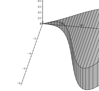
Figure 1: The curve $T_{F_{q}}$ in the $SO(3)$ manifold ($-1\leq q\leq 1$)

The left - right axis is in the $(+-)$-direction while the vertical is along $(-+)$ (the axes are marked in degrees). The points of the curve are projected down to the $(+-,00)$-plane and back to the $(+-,-+)$-plane (at equal intervals in $q$) for clarity of presentation. To find the value $q_{s}$ at which the curve meets the surface of the ball, we substitute (27) in (26), set $\theta^{(3)}_{q}$ equal to $\pi$ and solve for $q_{s}$ - the result is $q_{s}=-1$. The corresponding rotation matrix has $(1,-1,1)$ along the second diagonal as its only nonzero entries. The curve starts (for $q=-1$) at the right part of the figure (upper edge of the ribbon), touching at that point the $(+-,-+)$-plane on the diagonal (notice the anisotropic scaling of the axes) as well as the surface of the $SO(3)$ ball. At $q=1$, $T_{F_{q}}$ is the unit matrix, which corresponds to the origin of the ball. Notice that the tangent to the curve at the origin is along the diagonal in the $(+-,-+)$-plane (the same holds at $q=-1$). The property ${(F_{q^{-1}})}_{12}={(F_{q})}_{21}$ reflects itself in the following symmetry of the curve: the points corresponding to $q$ and $q^{-1}$ are mapped into each other by central reflection and subsequent interchange of the $(+-)$, $(-+)$ axes (this allows one to picture the missing segments $-\infty<q<-1$ and $1<q<\infty$, which are omitted from figure 1 for clarity). Notice that the above two missing segments “touch” as $q\rightarrow\pm\infty$ since, in this limit, $T_{F_{q}}$ tends to the common value

$$T_{F_{\pm\infty}}=\frac{1}{\sqrt{6}}\left(\begin{array}[]{ccc}\sqrt{2}&\sqrt{2}&\sqrt{2}\\ -\sqrt{3}&0&\sqrt{3}\\ 1&-2&1\end{array}\right)\,.$$ (29)

As in the 2-dimensional case, the results are simplified when the crystal limit is used as reference point. We find

$$T_{F_{q0}}=\frac{1}{ab}\left(\begin{array}[]{ccc}1&qb&q^{2}a\\ -q(1+q^{2})&(1-q^{2})b&qa\\ q^{4}&-qb&a\end{array}\right)\,.$$ (30)

The corresponding $SO(3)$ curve (for $q$ in the interval $[-3,3]$) is plotted in figure 2. In this case, the lower left - upper right axis is along the $(+-)$ direction while the vertical is again along $(-+)$.

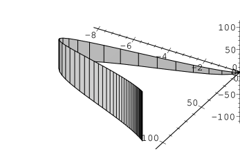
Figure 2: The curve $T_{F_{q0}}$ in the $SO(3)$ manifold ($-3\leq q\leq 3$)

The origin corresponds to $q=0$ while the point of the curve on the surface of the ball (not shown) to $q\rightarrow\pm\infty$.

A remark on the omission of $c$ from $\rho_{r}$ is in order at this point. It is sometimes desirable to know $F_{q}$ in the entire 16-dimensional space spanned by the bilinears in $c,\,x_{+},\,x_{0},\,x_{-}$. This, for example, could originate in the fact that although the quantum adjoint action closes linearly in the set $x_{+},\,x_{0},\,x_{-}$, the algebra of these three generators involves $c$. Such cases are easily handled noting that $F_{q}$ is simply a unit matrix in the 7-dimensional space we have omitted in the above computation.

4.3 The representation of the coproduct of ${\cal F}$

The method for computing $F_{q}$ used above is easily adapted to the computation of ${F_{q}}_{123}\equiv\rho_{r}^{\otimes 3}((\Delta\otimes\mathop{\rm id}){\cal F})$. The matrix $C_{123}=\rho_{r}^{\otimes 3}(\Delta^{(2)}{\cal C})$, where $\Delta^{(2)}({\cal C})\equiv(\Delta\otimes\mathop{\rm id})\circ\Delta({\cal C})$, is again symmetric and its eigenvectors are rotated by the orthogonal ${F_{q}}_{123}$ from their classical to their deformed position. This allows the computation of ${F_{q}}_{123}$ from a formula analogous to (18). Both $C_{123}$ and ${F_{q}}_{123}$ are of block-diagonal form, with each block acting in a subspace of fixed $H$-eigenvalue. Based on this observation, one easily sees that both matrices have 1, 3 and 6-dimensional blocks (two of each) and one 7-dimensional one. Blocks of equal dimension are equal to each other, up to (easily identified) permutations of rows and columns. We have carried out, with the help of MAPLE, the explicit computation of these matrices, with respect to the crystal limit (i.e. we have computed the matrix ${F_{q0}}_{123}\equiv{F_{q}}_{123}{F_{0}}_{123}^{-1})$. We present the (rather cumbersome) results in the appendix.

5 Applications

5.1 The universal $R$-matrix in the adjoint representation

The block diagonal form of the matrices involved simplifies significantly the computation of ${\bf R}\equiv\rho^{\otimes 2}_{r}({\cal R})$. Applying $\rho^{\otimes 2}_{r}$ in (15) gives

$${\bf R}=F_{q}^{\prime}\,\rho^{\otimes 2}_{r}(q^{{\bf t}})\,F_{q}^{-1}\,.$$ (31)

For the representation of the classical $R$-matrix we compute

$$\rho_{r}^{\otimes 2}({\bf t})=\{2,\,\left(\begin{array}[]{cc}0&2\\ 2&0\end{array}\right)\,,\left(\begin{array}[]{ccc}-2&-2&0\\ -2&0&-2\\ 0&-2&-2\end{array}\right)\}$$ (32)

which gives, upon exponentiation

$$\mu_{R_{c}}=q^{2},\qquad D_{R_{c}}=\frac{1}{2q^{2}}\left(\begin{array}[]{cc}q^{4}+1&q^{4}-1\\ q^{4}-1&q^{4}+1\end{array}\right)$$ (33)

as well as

$$T_{R_{c}}=\frac{1}{6q^{4}}\left(\begin{array}[]{ccc}q^{6}+3q^{2}+2&-2(q^{6}-1)&q^{6}-3q^{2}+2\\ -2(q^{6}-1)&2(2q^{6}+1)&-2(q^{6}-1)\\ q^{6}-3q^{2}+2&-2(q^{6}-1)&q^{6}+3q^{2}+2\end{array}\right)\,,$$ (34)

where $R_{c}\equiv\rho_{r}^{\otimes 2}({\cal R}_{c})$. We may now use (31) to find

$$\mu_{{\bf R}}=q^{2},\qquad D_{{\bf R}}=\left(\begin{array}[]{cc}1&q^{2}-q^{-2}\\ 0&1\end{array}\right),\qquad T_{{\bf R}}=\left(\begin{array}[]{ccc}q^{-2}&-q+q^{-3}&(q^{2}-q^{-2})(1-q^{-2})^{2}\\ 0&1&-q+q^{-3}\\ 0&0&q^{-2}\end{array}\right).$$ (35)

${\bf R}$ is seen to be upper triangular while $\hat{{\bf R}}\equiv P{\bf R}$ is symmetric ($P$ stands here for the permutation matrix, $P_{ij,kl}=\delta_{il}\delta_{kj}$ - $\hat{{\bf R}}$ is obtained from ${\bf R}$ by interchange of the rows of $D_{{\bf R}}$ and interchange of the first and third row of $T_{{\bf R}}$). One could also compute ${\bf R}$ starting from the known expression for ${\cal R}$, apply $\rho_{f}^{\otimes 2}$ to it and then conjugate with the tensor square of $A$ - the two results agree.

The characteristic equation for $\hat{{\bf R}}$ is easily computed now. Indeed, one finds that

$$(D_{\hat{{\bf R}}}-q^{2}I)(D_{\hat{{\bf R}}}+q^{-2}I)=0,\qquad(T_{\hat{{\bf R}}}-q^{2}I)(T_{\hat{{\bf R}}}+q^{-2}I)(T_{\hat{{\bf R}}}-q^{-4}I)=0\,.$$ (36)

Notice that $\mu_{\hat{{\bf R}}}$ and $D_{\hat{{\bf R}}}$ both satisfy the characteristic equation for $T_{\hat{{\bf R}}}$ - this implies that $\hat{{\bf R}}$ does too, i.e. $\hat{{\bf R}}$’s minimal polynomial is cubic. The characteristic polynomial for $\hat{{\bf R}}$ is obtained from its minimal one by raising its factors, in the order they appear above, to the powers 5, 3 and 1. Had we included $c$ in $\rho_{r}$, obtaining in this way a 16-dimensional matrix for $\hat{{\bf R}}$, the minimal polynomial would turn out to be quintic, the extra two factors being $(\hat{{\bf R}}-I)(\hat{{\bf R}}+I)$, coming from the $c$-sector in which $\hat{{\bf R}}$ is a permutation matrix. The above two factors would be raised to the power 3 and 4 respectively in the characteristic polynomial of $\hat{{\bf R}}$.

5.2 Quantum symmetrization

We consider here the problem of quantum symmetrization of identical particle states. We supply, for reasons of self-containment, a brief exposition of the relevant theory, along the lines of [7], which contains a thorough discussion.

As a first step towards the implementation of quantum group symmetries in quantum mechanics and quantum field theory, the question of the compatibility of Bose/Fermi statistics with quantum group actions ought to be addressed. Consider, for concreteness, a two (identical) particle system in quantum mechanics. The Hilbert space of the system is split into symmetric and antisymmetric subspaces, a division which is respected by the action of classical Lie algebra generators. This latter fact is traced to the symmetry of the classical coproduct under exchange of the two spaces, so that the classical permutation matrix $P$ commutes with the representation of the coproduct of the generators

$$[P,\rho^{\otimes 2}(\Delta_{c}(x))]=0,\qquad x\in U({\bf g}),$$ (37)

where ${\bf g}$ is the Lie algebra under consideration and $\rho$ the representation through which it acts on the one-particle states. In the quantum case, the lack of cocommutativity implies that the quantum group action mixes the two eigenspaces of $P$. The problem is rectified with the introduction of a quantum permutation operator $P^{F}$, given by conjugation by $F$ of the classical one, i.e.   $P^{F}=FPF^{-1}$. One easily shows that

$$[P^{F},\,\rho^{\otimes 2}(\Delta(x))]=0\,\qquad x\in U_{q}({\bf g})\,,$$ (38)

which guarrantees that quantum symmetric and antisymmetric states (defined as eigenstates of $P^{F}$) remain such after being acted upon by elements of $U_{q}({\bf g})$ (in the above equation, $F$ is computed in $\rho$).

Specifying ${\bf g}$, in the discussion above, to be $su(2)$ and working in the representation $\rho_{r}$, we find

$$S^{F}=\{1,\qquad\frac{1}{1+q^{4}}\left(\begin{array}[]{cc}1&q^{2}\\ q^{2}&q^{4}\end{array}\right),\qquad\frac{1}{1+q^{4}}\left(\begin{array}[]{ccc}q^{4}-q^{2}+1&q^{3}-q&q^{2}\\ q^{3}-q&q^{2}&-q^{3}+q\\ q^{2}&-q^{3}+q&q^{4}-q^{2}+1\end{array}\right)\}$$ (39)

while

$$A^{F}=\{0,\qquad\frac{1}{1+q^{4}}\left(\begin{array}[]{cc}q^{4}&-q^{2}\\ -q^{2}&1\end{array}\right),\qquad\frac{1}{1+q^{4}}\left(\begin{array}[]{ccc}q^{2}&-q^{3}+q&-q^{2}\\ -q^{3}+q&(q^{2}-1)^{2}&q^{3}-q\\ -q^{2}&q^{3}-q&q^{2}\end{array}\right)\}$$ (40)

where $S^{F}\equiv F\frac{1}{2}(1+P)F^{-1}$ and $A^{F}\equiv F\frac{1}{2}(1-P)F^{-1}$ are the quantum symmetrizer and antisymmetrizer respectively. In the $c$-sector, $S^{F}$ and $A^{F}$ are equal to their classical counterparts. Clearly, ${S^{F}}^{2}=S^{F}$ (similarly for $A^{F}$) and $S^{F}A^{F}=0$.

For systems with more than two identical particles one proceeds along similar lines. The quantum permutation matrix for adjacent spaces $i$, $i+1$ is given by $P^{F}_{i,i+1}={F_{q}}_{12\ldots n}P_{i,i+1}{F_{q}}^{-1}_{12\ldots n}$, where $P_{i,i+1}$ is the corresponding classical permutation matrix and ${F_{q}}_{12\ldots n}$ is the representation of $({\Delta}^{(n-1)}\otimes\mathop{\rm id}){\cal F}$ (different choices for ${F_{q}}_{12\ldots n}$ are possible). For example, for $n=3$, ${F_{q}}_{123}$ can be obtained from the crystal limit result of section 4 as ${F_{q}}_{123}={F_{q0}}_{123}{F_{10}}^{-1}_{123}$.

Appendix

We give here the explicit form for the 3, 6 and 7-dimensional blocks of ${F_{q0}}_{123}$, acting in the subspaces $(++0,+0+,0++)$, $(++-,+00,+-+,0+0,00+,-++)$ and $(+0-,+-0,0+-,000,0-+,-+0,-0+)$ respectively.

$${F^{(3)}_{q0}}_{123}=\frac{1}{mk}\left(\begin{array}[]{ccc}m&q^{4}k&-q^{6}\\ -q^{4}m&k&-q^{2}\\ 0&q^{2}k&k^{2}\end{array}\right)\,,$$

$${F^{(6)}_{q0}}_{123}=\left(\begin{array}[]{cccccc}y&-q^{3}w&q^{4}z&0&q^{8}r&q^{2}st^{2}\\ q^{3}3_{q^{2}}x^{2}y&2_{-q^{6}}w&-q^{-1}2_{q^{2}}z&-q^{2}x&-q^{3}2_{q^{2}}r&q2_{q^{4}}^{-1}s\\ 0&q^{3}w&q^{-4}z&0&r&s\\ q^{5}(1+3_{q^{2}})x^{2}y&q^{2}w&-q2_{q^{2}}z&x&(q-q^{7}+q^{9})r&-q^{-1}2_{q^{2}}st^{2}\\ -q^{4}3_{q^{2}}x^{2}y&-q^{4}w&-q^{-3}2_{q^{2}}z&q^{4}x&(q^{-1}-q+q^{7})r&(q2_{q^{4}})^{-1}s\\ (-q^{4}+q^{6}+q^{10})x^{2}y&0&z&q2_{q^{2}}x&-2_{q^{8}}r&q^{-2}st^{2}\end{array}\right)\,,$$

while ${F^{(7)}_{q0}}_{123}$ is given by

$$\left(\begin{array}[]{ccccccc}3_{q^{2}}^{-1/2}&q^{2}3_{-q^{4}}u&-q^{2}t&(-1+q^{4}+q^{6})d&e&(-q^{4}-q^{6}+q^{10})f&g\\ 0&(1-q^{2}+q^{6}+q^{8})u&q^{2}t&2_{-q^{4}}3_{q^{2}}d&q^{-4}e&q^{4}2_{q^{2}}^{2}f&0\\ 0&(q^{4}-q^{6}-q^{8})u&t&-3_{q^{2}}d&q^{2}e&(q^{2}-q^{6}-q^{8})f&g\\ q3_{q^{2}}^{-1/2}&(-q^{2}+q^{4}+q^{6})2_{-q^{4}}u&-q2_{-q^{2}}t&q^{-1}(2-5_{q^{2}})d&-q^{-3}2_{q^{2}}e&q^{3}(2+q^{2}-q^{4}-q^{6}+q^{8})f&-q^{-3}2_{-q^{4}}g\\ 0&(-q^{2}+q^{4}+q^{6})u&-q^{4}t&-q^{2}3_{q^{2}}d&q^{-6}e&(q^{4}-q^{8}-q^{10})f&-q^{-2}g\\ 0&-2q^{6}u&-q^{2}t&0&e&2_{q^{2}}2_{q^{8}}f&q^{-2}2_{-q^{4}}g\\ q^{2}3_{q^{2}}^{-1/2}&(-q^{2}-q^{4}+q^{6})u&q^{2}t&d&q^{-4}e&-q^{2}3_{-q^{4}}f&(2-3_{q^{2}})q^{-4}g\end{array}\right)\!\!.$$

We have used the notation $n_{x}\equiv 1+x+x^{2}+\ldots+x^{n-1}$ and

$$\begin{array}[]{rclcrcl}d&=&q(8_{q^{2}}3_{q^{2}})^{-1/2}&&e&=&q^{6}(2_{q^{4}}3_{-q^{2}}5_{-q}5_{q})^{-1/2}\\ f&=&(2_{q^{2}}2_{q^{4}}2_{q^{8}}5_{-q}5_{q})^{-1/2}&&g&=&q^{4}((1-q^{2}+q^{6}+q^{8})2_{q^{4}})^{-1/2}\\ k&=&\sqrt{2_{q^{8}}}&&m&=&\sqrt{3_{q^{4}}}\\ r&=&q(2_{q^{4}}2_{q^{8}}3_{-q}3_{q}3_{-q^{2}})^{-1/2}&&s&=&q^{2}\sqrt{\frac{3_{q^{2}}}{5_{q^{2}}}}\\ t&=&(5_{q^{2}}+q^{4})^{-1/2}&&u&=&((1-q^{2}+q^{6}+q^{8})2_{q^{4}}3_{q}3_{-q}3_{-q^{2}})^{-1/2}\\ w&=&4_{q^{4}}^{-1/2}&&x&=&(5_{q^{2}}+2q^{4})^{-1/2}\\ y&=&2_{q^{4}}^{2}3_{q}3_{-q}x^{2}&&z&=&q^{4}(3_{q}3_{-q}3_{-q^{2}}5_{-q}5_{q})^{-1/2}\,.\end{array}$$

References

- [1] M. Bonechi, R. Giachetti, E. Sorace and M. Tarlini “Deformation Quantization of the Heisenberg Group” Comm. Math. Phys. 169 (1995) 627-634
- [2] T.L.Curtright “Deformations, Coproducts, and ”, in Quantum Groups, T.L. Curtright, D.B. Fairlie and C.K.Zachos eds., World Scientific 1991
- [3] T.L. Curtright, G.I. Ghandour and C.K. Zachos “Quantum Algebra Deforming Maps, Clebsch-Gordan Coefficients, Coproducts, and Matrices”, J. Math. Phys. 32 (3) (1991) 676
- [4] L. Dabrowski, F. Nesti and P. Siniscalco “On the Drinfeld Twist for Quantum ”, preprint SISSA 130/96/FM, q-alg/9610012
- [5] V.G. Drinfeld, “Quasi-Hopf Algebras”, Leningrad Math. J. 1 (1990) 1419
- [6] R.A. Engeldinger “On the Drinfeld-Kohno Equivalence of Groups and Quantum Groups”, preprint LMU-TPW 95-13, q-alg/9509001
- [7] G. Fiore and P. Schupp “Identical Particles and Quantum Symmetries”, preprint LMU-TPW 95-10, hep-th/9508047 v3
- [8] C.K. Zachos “Quantum Deformations”, in Quantum Groups, T.L. Curtright, D.B. Fairlie and C.K.Zachos eds., World Scientific 1991