Iso-topological relaxation, coherent structures, and Gaussian turbulence in two dimensional magnetohydrodynamics

Abstract

The long-time relaxation of ideal two dimensional (2D) magnetohydrodynamic (MHD) turbulence subject to the conservation of two infinite families of constants of motion—the magnetic and the “cross” topology invariants—is examined. The analysis of the Gibbs ensemble, where all integrals of motion are respected, predicts the initial state to evolve into an equilibrium, stable coherent structure (the most probable state) and decaying Gaussian turbulence (fluctuations) with a vanishing, but always positive temperature. The non-dissipative turbulence decay is accompanied by decrease in both the amplitude and the length scale of the fluctuations, so that the fluctuation energy remains finite. The coherent structure represents a set of singular magnetic islands with plasma flow whose magnetic topology is identical to that of the initial state, while the energy and the cross topology invariants are shared between the coherent structure and the Gaussian turbulence. These conservation laws suggest the variational principle of iso-topological relaxation which allows us to predict the appearance of the final state from a given initial state. For a generic initial condition having $x$ points in the magnetic field, the coherent structure has universal types of singularities: current sheets terminating at $Y$ points. These structures, which are similar to those resulting from the 2D relaxation of magnetic field frozen into an ideally conducting viscous fluid, are observed in the numerical experiment of D. Biskamp and H. Welter [Phys. Fluids B 1, 1964 (1989)] and are likely to form during the nonlinear stage of the kink tearing mode in tokamaks. The Gibbs ensemble method developed in this work admits extension to other Hamiltonian systems with invariants not higher than quadratic in the highest-order-derivative variables. The turbulence in two dimensional Euler fluid is of a different nature: there the coherent structures are also formed, but the fluctuations about these structures are non-Gaussian.

52.35.Ra, 47.25.Cg.

I Introduction

Turbulence in two dimensional fluids is simple enough to allow some analytically tractable models [1, 2, 3, 4] and high-resolution computation [5, 6, 7, 8, 9], but still sufficiently complex to exhibit the general challenging nature of turbulence. In addition, many features of plasma and geophysical fluid dynamics are essentially two dimensional.

The principal difficulty encountered by any analytical approach to fluid turbulence is that the underlying equations of motion are nonintegrable, a quality independent of the abilities of the researcher. To overcome this difficulty, two major analytical approaches have been attempted so far, namely, (a) statistical closures dealing with simplifying, but usually uncontrollable, modifications of the dynamical equations and (b) considerations of a priori equally probable states constrained by the known integrals of motion. In this work we take the second approach, where the consistency requirement is to allow for all constants of the motion.

The conventional Boltzmann-Gibbs statistical mechanics, when applied to partial differential equations [10, 11, 12, 13], encounters a fundamental obstacle because of the underlying infinite number of degrees of freedom and the necessity to use a finite ($N$) dimensional approximation. The continuum limit $N\to\infty$, in common to all classical fields, results in the so-called ultraviolet catastrophe (the divergence of energy at finite temperature), a problem which goes back to Jeans. Unlike the equilibrium electromagnetic radiation, the ultraviolet catastrophe in fluid turbulence cannot be remedied by quantization and should be resolved within the classical framework. The tendency toward the equipartition of energy between the degrees of freedom (by $T/2$ for each degree, where $T$ is the energy temperature) in a closed continuum system can only be satisfied by letting the temperature to zero. In fact, the way the temperature goes to zero as the number of degrees of freedom goes to infinity is the heart of the problem. Nontrivial equilibrium states are obtained when there are more than one integrals of motion, which diverge at different rates as $N\to\infty$.

The absence of a well-defined concept of measure in a functional (infinite dimensional) space requires an $N$ dimensional discretization, even though the final results are obtained by letting $N\to\infty$. Lee [14] was the first to use the truncated Fourier series to show the validity of an infinite dimensional Liouville theorem. The choice of the discrete variables is not unique, and one ought to make sure that the results of the statistical theory of turbulence be invariant with respect to the way this choice is made.

A less formal, physical motivation for the discretization procedure can be found in the finiteness of the number $N(t)$ of the “effectively excited” collective modes at any finite time $t$. Under “effectively excited” we mean modes with amplitudes not yet exponentially small (a smooth field, for instance, has exponentially small high Fourier harmonics). There are examples of $N(t)$ becoming infinite in finite time [15], even when a real-space collapse [16] does not occur. It appears, however, that in two dimensional ideal hydrodynamics and magnetohydrodynamics $N(t)$ behaves algebraically, $N(t)\simeq(t/{\tau}_{A})^{p}$, so that the time of the doubling of $N(t)$ is of order $t$ and the time of the increment of $N(t)$ by one is of order ${\delta}t={\tau}_{A}(t/{\tau}_{A})^{1-p}$, if $0<p<1$. Hence, on time scale longer than the eddy turnover (nonlinear mode interaction) time ${\tau}_{A}$, one may expect an equilibrium statistical distribution among the effectively excited $N(t)$ modes. By letting $N(t)\gg 1$ in this distribution, we shall infer the most probable direction of the long-time system evolution. The probability of a deviation from the most probable state goes to zero as the number of degrees of freedom goes to infinity. As for a continuum conservative system we really mean $N(t)\to\infty$ as $t\to\infty$, the probabilistic nature of the statistical prediction assumes a rather deterministic quality.

Artificial finite dimensional approximations are notorious for destroying an infinity of topological invariants (also known as freezing-in integrals or Casimirs), which impose important constraints on the evolution. An interesting alternative proposed by Zeitlin [17], whereby an $N$ dimensional hydrodynamic-type system conserves $\sim\sqrt{N}$ invariants, is not quite suitable for continuum fields because of the implied periodicity in the Fourier space corresponding to modulated point vortices in real space. It would be very interesting to construct other “meaningful” (that is, having many invariants) finite-mode hydrodynamics with well-behaved real-space velocity fields.

So far, most statistical theories of continuum hydrodynamics, most notably the absolute equilibrium ensemble (AEE) theory [18, 19, 20], simply ignored all topological invariants except quadratic ones, such as enstrophy and helicity in hydrodynamics or magnetic helicity, cross helicity, and square vector potential (in two dimensions) in magnetohydrodynamic turbulence. These integrals were honored the special attention in part because of their ruggedness (survivability under the approximation of a finite number of Fourier modes), but mostly because of the convenience to handle quadratic integrals.

Despite the dissatisfaction with such a reasoning (cf. [21]), the attempts to incorporate all topological invariants in Gibbs statistics have been less frequent, the examples including Vlasov-Poisson system [22] and 2D Euler turbulence [3, 23, 24, 25]. For the reasons discussed in Sec. VI and Appendix D, these attempts appear not quite successful, because the non-Gaussianity of turbulent fluctuations in these systems poses a fundamental difficulty in making quantitative predictions about the equilibrium turbulent states. The key problem is that the averaging with respect to the given probability functional of a turbulence involves integration in a functional (infinite dimensional) space. These averages are well defined—that is, independent of the discretization procedure involved, if and only if the probability functional is Wienerian, or Gaussian in the highest-order derivative [26]. Otherwise, the result of the averaging is sensitive to the arbitrary choice of the sequence of discrete representations, which makes such probability functionals ambiguous, to say the least. In the present work we point out that these difficulties are absent from a certain class of systems; namely, those where all integrals of motion are not higher than quadratic in the highest-order-derivative variable. Important examples of such systems, allowing a valid Gibbs-ensemble description of turbulence, include two dimensional and reduced magnetohydrodynamics.

The problem of accounting for all invariants is circumvented by the representation of turbulence in the form of a gas of point vortices, which is a very singular, and very special topologically, although an asymptotically exact solution of the hydrodynamic equations. The localization of vorticity in point vortices makes the topological constraints trivially fulfilled for any motions. The conservation of only energy and the Liouville theorem expressed in the convenient form of the spatial variables of the vortices yield nicely to the statistical mechanical description, although the thermodynamic limit of infinitely many point vortices has long been a controversial issue [1, 27, 28, 29, 30]. It remains unclear to what extent the gas of many point vortices represents a continuum two dimensional turbulence. The frustrating dependence of the statistics of point vortices on the arbitrary choice of their strengths was noted by Onsager and reflects the above-mentioned fundamental difficulty in the 2D Euler turbulence.

We pursue an analytical approach to continuum two dimensional ideal MHD turbulence where all topological invariants are respected. We use the Gibbs ensemble analysis to predict the following evolution of the turbulence. An initial state evolves into (a) a stationary, stable coherent structure, which appears as the “most probable state” and (b) small-scale turbulence (fluctuations) with Gaussian statistics. The Gaussianity of the MHD fluctuations was recently numerically confirmed by Biskamp and Bremer [31]. At large time the fluctuations of the magnetic flux and the fluid stream function assume vanishing amplitude and length scale (while containing finite energy and dominating phase volume), and become essentially invisible on the background of the coherent structure. In this sense, the coherent structure can be regarded as an attractor or a relaxed state, although the underlying dynamics is perfectly Hamiltonian.

The concept of “statistical attractor,” introduced by Vladimir Yankov [32, 33, 34], emphasizes the method of analysis and describes this kind of Hamiltonian relaxation, when the excess of phase-space volume and energy get hidden in obscure (small-scale) corners of the infinite dimensional phase space. The fundamental difference between the statistical attractors in nonintegrable wave-type systems [32, 33, 34, 35] (where there are only a finite number of integrals of motion) and the hydrodynamic-type systems (where the number of integrals is infinite) is the universal shape of the attractor—soliton—in the first case, and the nonuniversal shape of the coherent structure—vortex—in the second case. The appearance of the coherent structure depends on the initial condition, but is the same for all initial conditions with identical topological invariants [Eqs. (6) and (7)]. In this sense, the asymptotically emerging coherent structures (relaxed states) in hydrodynamic systems are attractors only within a certain subclass (basin) of initial conditions. These relaxed states can be called topological attractors.

The specific of two dimensional MHD is that the coherent structure inherits from the initial state all magnetic topology invariants, but only a fraction of energy, the rest of which goes to the Gaussian fluctuations. These invariant sharing properties can be interpreted in terms of the well-known reasoning of turbulent cascades. In the case of 2D MHD the energy cascade is direct (i.e., toward the small-scale fluctuations), while the magnetic topology cascades inversely (toward a large-scale magnetic structure). However, compared to the cascade description, the invariant sharing properties appear to present a clearer physics of what happens to the conserved quantities in a closed turbulent system. In fact, this allows us to predict the appearance of the relaxed state, which should minimize energy subject to certain topological constraints. One of the novelties of our analysis is using a second functional set of “cross” topology invariants [36, 37], which was not used in MHD turbulence theories so far, including the previous note [38]. We find that these invariants have an important effect on the statistical description of turbulence; specifically, the shape of the coherent structure is sensitive to the cross topology invariants. In many features our development is analogous to the Gibbs ensemble treatment of the truncated Fourier representation of 2D MHD which was investigated by Fyfe and Montgomery [20]. The reason for this resemblance is partial consistency of the Gibbs statistics with partial invariants accounting. In fact, our theory shows that truncated 2D MHD equations partially represent the true statistics of ideal 2D MHD.

Unlike neutral fluid dynamics, magnetohydrodynamics in two dimensions are known to produce energetic small scales. This makes the difference between 2D and 3D for MHD turbulence less drastic than that for fluid turbulence. In our model, we observe two types of small-scale behavior: (a) for a generic (that is, topologically nontrivial) initial condition, the coherent structure must have discontinuities in the form of current sheets and (b) the Gaussian fluctuations in the long evolved state have both vanishing length scale and amplitude so that the gradients and the energy are finite. The numerically observed current-sheet-type structures [5] are explained by our theory as the singular coherent structures.

The paper is organized as follows. In Sec. II we present the equations and the constants of the motion. In Sec. III we discuss the stationary solutions of the MHD equations and formulate the Arnold variational principle in the form suitable for 2D MHD. In Sec. IV the canonical ensemble approach to MHD turbulence is set forth (Sec. IV.A), and the most probable state (Sec. IV.B) and the fluctuations about this state (Sec. IV.C) are analyzed. The key issue of how the integrals of motion are divided between the coherent structure and the fluctuations is addressed in Sec. IV.D. In Sec. V we reformulate the properties of the coherent structure using a variational principle of iso-topological relaxation, which allows us to predict the appearance of the structure. This prediction is then compared with numerical results (Sec. V.A). In Sec. V.B we speculate on the role of small dissipation and the relation between the resistive and the ideal MHD relaxation in the kink tearing mode in tokamaks. Section VI restates the principal steps of our statistical method and summarizes our work. Some technical details and results not directly related to MHD turbulence are set in Appendices. In Appendix A we discuss the Lyapunov stability of MHD and Euler fluid equilibria and point out the relation of minimum- and maximum-energy stability to positive- and negative-temperature Gibbs states, respectively. Appendix B addresses the Liouvillianity of the eigenmodes that we use in the Gibbs statistics. In Appendix C the spectrum of the eigenmodes is studied. In Appendix D we discuss the application of the Gibbs-ensemble formalism to the turbulence of two dimensional Euler fluid.

II Equations and constants of the motion

We consider the set of equations of two dimensional incompressible ideal magnetohydrodynamics (cf. [39])

$${\partial}_{t}a = \{{\psi},a\}\ ,$$ (1)

$${\partial}_{t}{\omega} = \{{\psi},{\omega}\}+\{j,a\}\ ,$$ (2)

where $\{A,B\}\equiv{\mbox{\boldmath$\bf\nabla$}}A\times{\mbox{\boldmath$\bf\nabla$}}B\cdot{\widehat{{\bf z}}}$ denotes the Poisson bracket, ${\widehat{{\bf z}}}$ the unit vector in the $z$ direction, ${\psi}(x,y,t)$ the stream function of the fluid velocity field ${\bf v}={\mbox{\boldmath$\bf\nabla$}}\times({\psi}{\widehat{{\bf z}}}),\;{\omega}=-{\mbox{\boldmath$\bf\nabla$}}^{2}{\psi}$ the fluid vorticity, $a(x,y,t)$ the normalized vector potential of the magnetic field ${\bf B}=(4\pi{\rho})^{1/2}{\mbox{\boldmath$\bf\nabla$}}\times(a{\widehat{{\bf z}}})$ (${\rho}$ being the constant fluid density), and $j=-{\mbox{\boldmath$\bf\nabla$}}^{2}a$ the normalized electric current flowing perpendicular to the $(x,y)$ plane. The boundary conditions $a={\psi}=0$ are assumed at a rigid boundary encompassing the finite domain with the area ${\cal S}$.

The incompressibility of the fluid motion is a reasonable approximation in tokamaks where the strong toroidal magnetic field $B_{z}$ makes plasma compression energetically expensive. In the reduced MHD approximation [40, 41, 42], where the fast Alfvén and magnetosonic waves due to $B_{z}$ are ignored, the strong uniform field $B_{z}$ drops out of the equations of the motion.

The system (1)—(2) conserves the following quantities: the energy

$$E=E_{m}+E_{f}=\frac{1}{2}\int\left[({\mbox{\boldmath$\bf\nabla$}}a)^{2}+({\mbox{\boldmath$\bf\nabla$}}{\psi})^{2}\right]\,d^{2}{\bf x}=\frac{1}{2}\int\left(aj+{\psi}{\omega}\right)\,d^{2}{\bf x}\ ,$$ (3)

consisting of the magnetic part $E_{m}$ and the fluid part $E_{f}$, the momentum (with translationally invariant, or in the absence of, boundaries)

$${\bf P}=\int{\bf v}\,d^{2}{\bf x}=\frac{1}{2}\int{\bf x}\times{\widehat{{\bf z}}}{\omega}\,d^{2}{\bf x}\ ,$$ (4)

the angular momentum (with circular or no boundaries)

$$M{\widehat{{\bf z}}}=\int{\bf x}\times{\bf v}\,d^{2}{\bf x}=\frac{1}{3}\int{\bf x}\times({\bf x}\times{\widehat{{\bf z}}}{\omega})\,d^{2}{\bf x}\ ,$$ (5)

the magnetic topology invariants

$$I_{F}=\int F(a)\,d^{2}{\bf x}\ ,$$ (6)

and the “cross” topology invariants

$$J_{G}=\int{\omega}G(a)\,d^{2}{\bf x}=\int G^{\prime}(a){\mbox{\boldmath$\bf\nabla$}}{\psi}\cdot{\mbox{\boldmath$\bf\nabla$}}a\,d^{2}{\bf x}\ ,$$ (7)

where $F$ and $G$ are arbitrary functions. Along with the continuum set of integrals (6) and (7), we will also use their discretized analogues,

$$I_{n} = \int a^{n}\,d^{2}{\bf x}\ ,$$ (6a)

$$J_{n} = \int{\omega}a^{n}\,d^{2}{\bf x}\ ,$$ (7a)

through which the continuum invariants can be Taylor expanded.

Strictly speaking, invariants (6) and (7) do not yet imply the conservation of topology. Equation (6) only means that allowed motions are incompressible interchanges of fluid elements together with their “frozen” values of the magnetic flux $a$. The topology of the contours of $a$ will be conserved only if these interchanges are performed by continuous movements, a constraint which is not built into Eq. (6) but follows from the equations of motion for smooth initial conditions. Then the conservation of magnetic topology expressed by Eq. (6) means that if the contour $a(x,y)=a_{1}$ initially lies inside the contour $a(x,y)=a_{2}$, then this topological relation is preserved by the motion; if a contour of $a$ has a hyperbolic (saddle, $x$) point, this quality will also persist. In addition to the topological constraints, the integrals (6) also specify the incompressibility of the fluid, so that the area inside a given contour of $a$ remains constant. The geometrical meaning of the integrals (7) is that the amount of the fluid vorticity ${\omega}$ on a given contour of $a$ (to be more precise, the integral of ${\omega}$ over the anulus between two infinitesimally close contours) is conserved. Although stating nothing of the contours of ${\omega}$ or ${\psi}$, the conservation of the integrals (7) also bears certain topological relation between the magnetic field and the vorticity field, which motivates our notation of the “cross topology invariants.”

The invariants $J_{G}$ appear to be poorly known, although the particular member of the family (7a)—the cross helicity

$$J_{1}=\int{\omega}a\,d^{2}{\bf x}=\frac{1}{\sqrt{4\pi{\rho}}}\int{\bf v}\cdot{\bf B}\,d^{2}{\bf x}$$ (8)

—has been extensively discussed in the literature. The invariants (7) were first noted by Morrison and Hazeltine [36]. Independently, a similar set of integrals was used to study the vortex stability in the framework of two dimensional electron MHD [37]. The idea towards the existence of a second set of topological invariants is suggested by the observation that there is another frozen-in quantity, namely the vorticity ${\omega}$, in the Euler limit $a\equiv 0$, which must have a counterpart in the MHD case $a\neq 0$. Once the existence of a second functional set of invariants is suspected, it is not hard to guess the form of the topological invariants (7). Although this is not straightforward, one can trace the transition, as $a\to 0$, from Eqs. (6) and (7) to the Euler invariants $\int F({\omega})\,d^{2}{\bf x}$.

Another way to find the topological invariants is to identify the Hamiltonian structure using a noncanonical Poisson bracket [36], whereby the topological invariants appear as Casimirs.

III MHD equilibria and Arnold’s variational principle

The system of equations (1)—(2) has stationary solutions satisfying

$$\{{\psi},a\} = 0\ ,$$ (9)

$$\{{\psi},{\mbox{\boldmath$\bf\nabla$}}^{2}{\psi}\} = \{a,{\mbox{\boldmath$\bf\nabla$}}^{2}a\}\ .$$ (10)

The equilibrium condition can be rewritten in a more convenient form by substituting the functional dependence ${\psi}={\psi}(a)$, which is implied by Eq. (9), into Eq. (10). Then, after simple manipulations, we find

$$\{{\Psi}(a),{\mbox{\boldmath$\bf\nabla$}}^{2}{\Psi}(a)\}=0\ ,$$ (11)

where

$${\Psi}(a)=\int_{0}^{a}da^{\prime}\sqrt{\pm\left(1-[d{\psi}(a^{\prime})/da^{\prime}]^{2}\right)\,}\ ,$$ (12)

and the sign is chosen to make the square root real. As equation (11) shows, any two dimensional MHD equilibrium with fluid flow (${\psi}\neq 0$) is reduced to a purely magnetic (${\psi}=0$) equilibrium for a modified magnetic vector potential $a^{\prime}={\Psi}(a)$. Note that the magnetic field lines (the contour lines of the vector potential) are identical for both the true field $a$ and the modified field $a^{\prime}$, although the values of $a$ and $a^{\prime}$ on these lines are different.

The most evident stationary solution is given by an arbitrary circular distribution ${\psi}={\psi}(r),\;a=a(r)$, where $r$ is the distance from the origin. Another solution to (9)—(10) corresponds to the identical zero in one of the Elsässer variables, where ${\psi}(x,y)\equiv\pm a(x,y)$ is an arbitrary function of $x$ and $y$, so that ${\Psi}(a)\equiv 0$. For the case when $|{\psi}|$ and $|a|$ are not identical, there exist many periodic and quasiperiodic solutions in the form

$$C{\psi}({\bf x})=a({\bf x})=\sum_{m=1}^{N}A_{m}\cos({\bf k}_{m}{\bf x}+\theta_{m})\ ,$$ (13)

where the moduli of the wavevectors ${\bf k}_{m}$ are the same. In addition to the smooth solutions one can devise a wide class of singular solutions with appropriate boundary conditions at the lines of discontinuity. Without additional physical constraints, such as stability or topology, the class of all equilibria is too wide to be useful. In Secs. IV and V we provide such constraints, which specify the physically interesting (attracting) equilibria. In many cases these equilibria must be singular.

There exists a profound relation between the stationary solutions and the constants of the motion. For finite dimensional conservative systems, the D’Alembert variational principle says that the energy variation be zero at an equilibrium. For a hydrodynamic-type conservative system, the counterpart of the D’Alembert theorem is the Arnold variational principle. Originally formulated for the Euler equation, but carried over without difficulty to other hydrodynamics, the principle states that at a stationary (and only stationary) solution the variation of energy, subject to the conservation of all topological invariants, be zero:

$${\delta}E\bigg{|}_{I_{F},J_{G}={\rm const},\ \forall F{\ \rm and\ }G}=0\ .$$ (14)

If, in addition, the second variation is definite—that is, the energy assumes a nondegenerate conditional extremum, then the equilibrium is Lyapunov stable. In fact, this was the search for stable fluid flows which motivated Arnold’s work. The power of the method lies in the possibility to write the general iso-topological (iso-vortical in Arnold’s notation) variation in a closed form. When all the integrals (6) and (7) are to be conserved, such a variation is

$${\Delta}\left(\begin{array}[]{l}a\\ {\omega}\end{array}\right)={\delta}\left(\begin{array}[]{l}a\\ {\omega}\end{array}\right)+\frac{1}{2!}{\delta}^{2}\left(\begin{array}[]{l}a\\ {\omega}\end{array}\right)+\ldots\ ,$$ (15)

where the infinitesimal iso-topological variation is given by [37]

$${\delta}\left(\begin{array}[]{c}a\\ {\omega}\end{array}\right)=\left(\begin{array}[]{c}\{\mu,a\}\\ \{\mu,{\omega}\}+\{\nu,a\}\end{array}\right)\ ,$$ (16)

$\mu(x,y)$ and $\nu(x,y)$ being arbitrary functions. The operator of finite variation ${\Delta}$ can be symbolically expressed through the infinitesimal variation ${\delta}$ as

$${\Delta}=\exp{\delta}-1\ .$$ (17)

It is easy to verify that the finite variation (15) conserves both sets of integrals $I_{F}$ and $J_{G}$ to all orders in $\mu$ and $\nu$. The form of the variation is suggested by the form of Eqs. (1)—(2), where one can substitute the quantities ${\psi}$ and $j$ by arbitrary ${\partial}\mu/{\partial}t$ and ${\partial}\nu/{\partial}t$, respectively, to preserve only the Poisson-bracket structure of the equations and thereby to iso-topologically (that is, at constant $I_{F}$ and $J_{G}$) drag the fields $a$ and ${\omega}$ to a new state, where the values of all other integrals, if any, are generally different from those of the initial state.

Let us see what happens to the energy (3) under the variation (15)—(16). Writing the total change in the energy in the form ${\delta}E+{\delta}^{2}E/2!+\ldots$, we obtain after integrating by parts

$${\delta}E=-\int[\mu\left(\{{\psi},{\omega}\}+\{j,a\}\right)+\nu\{{\psi},a\}]\,d^{2}{\bf x}\ .$$ (18)

By requiring that the first energy variation (18) be zero for all $\mu$ and $\nu$ we arrive exactly at the system of equations (9)—(10) specifying the equilibrium solution. This strongly suggests that the two sets of the topological invariants (6) and (7) are indeed complete, a condition necessary to apply statistics (Sec. IV) in a meaningful way.

The second iso-topological variation of energy can be used to investigate the stability of MHD equilibria, as discussed in Appendix A.

IV Gibbs statistics of two dimensional MHD turbulence

We now wish to analyze the long-time evolution of the system subject to Eqs. (1) and (2) for a given initial condition $a_{0}({\bf x}),\;{\psi}_{0}({\bf x})$. The probability distribution functional $P[a({\bf x}),{\psi}({\bf x})]$ can serve this purpose. This functional specifies the relative probability, with respect to time measure, of the spatial behaviors of various states $a({\bf x},t)$ and ${\psi}({\bf x},t)$. As $P$ is invariant under the evolutional change of the fields $a$ and ${\psi}$, it must be a function of the constants of motion (3)—(7).

IV.A Choice of statistical ensemble

For a conservative Hamiltonian system, $P$ is given by the microcanonical ensemble,

$$P_{MC}[a,{\psi}]={\delta}(E[a,{\psi}]-E_{0})\,\prod_{n}{\delta}(I_{n}[a,{\psi}]-I_{n0})\,{\delta}(J_{n}[a,{\psi}]-J_{n0})\ ,$$ (19)

specifying a uniform distribution on the manifold of the specified (initial) integrals of motion. It must be emphasized that the validity of the microcanonical ensemble requires at least four assumptions.

1. The phase space must be finite dimensional; that is, the fields $a$ and ${\psi}$ are parameterized by discrete dynamical variables $f_{m},\ m=1,2,\ldots,N$, so that the concept of measure in the space of states is meaningful. This is a tricky issue as to how many variables are needed (see discussion in Sec. I).

2. The motion on the manifold of conserved invariants is nonintegrable (chaotic). The fundamental phenomenon lying behind the ergodic behavior (uniform distribution over the manifold) is Hamiltonian chaos, whose principal manifestation is the exponential divergence of nearby trajectories. The chaotic motion is possible only if the dimension of the manifold ($N-N_{I}$, where $N_{I}$ is the number of invariants) is three or more (four or more to allow the Arnold diffusion, so that all of the manifold might be visited by each trajectory). The property of ergodicity was proved for very special cases [43] but is believed to be generally valid if the dimension of the manifold is sufficiently large: $N-N_{I}\gg 1$. The remarkable accuracy of the classical thermodynamics is connected with the macroscopic numbers of degrees of freedom ($N\sim 10^{23}$) and only a few invariants. It is also natural to expect that the microcanonical statistics will work in turbulence (which can be loosely defined as chaos in PDE), where the limit $N\to\infty$ should be carefully taken.

3. The manifold of conserved integrals specified by the delta functions in (19) must be connected. The problem of connectivity of complicated iso-surfaces is related to the percolation problem [44]. The percolation threshold, above which the connectivity takes place, is inversely proportional to the dimension of the iso-surface. This suggests that in the continuum (infinite dimensional) limit the connectivity of the manifold of conserved integrals should not be a problem.

4. The dynamical variables $f_{m}(t)$ must satisfy the Liouville theorem: $\sum_{m}{\partial}\dot{f}_{m}/{\partial}f_{m}=0$. For non-Liouvillian variables a weighting factor (the Jacobian of change to Liouvillian variables) should be included in Eq. (19).

In a hydrodynamic-type system, where the number of dynamical constraints is infinite, we encounter another difficulty. Namely, any attempt to restrict the dimension of the phase space without restriction on the number of conserved quantities immediately drives the manifold of conserved integrals into an empty set, where no mixing may occur. Motivated by the experimental/numerical observation that turbulence does exist, as well as by the functional arbitrariness of the iso-topological variation (16), we adopt a hypothesis that there exists a “meaningful” $N$ dimensional MHD approximation with at most $N_{I}(N)$ conserved integrals, where both $N_{I}$ and $N-N_{I}$ go to infinity as $N\to\infty$. (In Zeitlin’s example [17] for the Euler fluid $N_{I}\simeq N^{1/2}$.) The specific form of this approximation is unimportant for our arguments.

The microcanonical ensemble (19) is inconvenient to handle and is commonly transformed into the more convenient canonical (Gibbs) ensemble by integrating $P_{MC}$ over most of the dynamical variables in the amount of $N_{th}\gg N-N_{th}\gg 1$. These $N_{th}$ degrees of freedom can referred to as “thermal bath.” The integration over the thermal bath variables leads to an exponential dependence of the resulting distribution on the integrals of motion expressed through the remaining $N-N_{th}$ variables, the rest of the information being stored in arbitrary constants called temperatures.

In our problem, the dimension $N^{\prime}=N-N_{th}$ of the subsystem can be also taken large, which amounts to another finite dimensional ($N^{\prime}$) MHD approximation. However, now we have the canonical distribution over the remaining $N^{\prime}$ variables,

$$P[a,{\psi}]=\exp\left[-{\alpha}\left(E[a,{\psi}]+\sum_{n}{\beta}_{n}I_{n}[a]+\sum_{n}{\gamma}_{n}J_{n}[a,{\psi}]\right)\right]\ ,$$ (20)

instead of the microcanonical one (19). A drastic simplification achieved by the change of the ensemble is that in the finite dimensional Gibbs distribution (20), where the fields $a$ and ${\psi}$ are parameterized by $N^{\prime}$ modes and the summation over invariants runs up to $N_{I}(N^{\prime})$, we may extend the summation up to infinity without significant change in the result, which was impossible for the product of delta functions in the microcanonical ensemble (19).

In Eq. (20), the constants ${\alpha},\;{\alpha}{\beta}_{n}$ and ${\alpha}{\gamma}_{n}$ appear as the reciprocal temperatures corresponding to each invariant. These constants are to be determined from the initial state by solving the infinite system of equations:

$$\left<E\right>_{P}=E_{0}\ ,\quad\left<I_{n}\right>_{P}=I_{n0}\ ,\quad\left<J_{n}\right>_{P}=J_{n0}\ ,\quad n=0,1,2,\ldots\ ,$$ (21)

expressing the conservation of the integrals of motion. Here the subscript “0” refers to the initial state. As a result of solving Eqs. (21), each parameter ${\alpha},\;{\beta}_{n},$ or ${\gamma}_{n}$ ($n=0,1,2,\ldots$) is a function of the infinity of the initial invariants $E_{0},\;I_{n0}$ and $J_{n0}$. It is emphasized that there is no arbitrariness in the temperatures characterizing the Gibbs distribution of a closed system. In fact, this is the central problem in our theory how to determine these temperatures in order to predict the final state from the given initial state.

The angular brackets in Eqs. (21) denote the ensemble averaging,

$$\left<A\right>_{P}=\frac{\int A\,P[a,{\psi}]{\cal D}a{\cal D}{\psi}}{\int P[a,{\psi}]{\cal D}a{\cal D}{\psi}}\ ,$$ (22)

which involves functional integrals over the space of the system states. This kind of integrals do not always exist. However, when the probability functional $P$ is Gaussian, the functional integrals belong to the important class of Wiener integrals [45] (their complex counterparts are known as path integrals [46]), which are soluble and well-behaved. This is exactly what we use in order to resolve the ultraviolet catastrophe. In fact, we seek the long evolved state in the form of a coherent structure plus small-amplitude fluctuations. This allows us to expand the integrals in the exponential (20) about the coherent structure up to quadratic terms, which will result in a Gaussian probability functional.

The uniform and additive (with respect to the eigenmodes) invariants is another assumption lying behind the transition from the microcanonical (19) to the canonical (20) distribution functionals. The additivity of the invariants can be achieved by the procedure of diagonalization, which only works for quadratic forms.

In the spirit of the conventional statistical mechanics we call the state specified by the detailed list of variables $(f_{1},\ldots,f_{N})$ the microstate, whereas the union of all microstates with the same $(f_{1},\ldots,f_{N^{\prime}}),\ N^{\prime}\ll N$ the macrostate. The entropy $S$—a functional of the macrostate—is then introduced as the logarithm of the number of various microstates corresponding to the given macrostate. Up to an additive constant, $S$ is the logarithm of the microstate phase volume on the manifold (19):

$$S[f_{1},\ldots,f_{N^{\prime}}]=\ln\int P_{MC}[f_{1},\ldots,f_{N}]\,df_{N^{\prime}+1}\ldots df_{N}\ .$$ (23)

In other words, the entropy is simply the logarithm of the canonical distribution functional (20),

$$S[a,{\psi}]=\ln P[a,{\psi}]=-{\alpha}(E[a,{\psi}]+I_{\beta}[a]+J_{\gamma}[a,{\psi}])\ ,$$ (24)

if $N^{\prime}\gg 1$. In Eq. (24), the integrals $I_{\beta}$ and $J_{\gamma}$ are defined by Eqs. (6) and (7), respectively, and the functions

$${\beta}(a)=\sum_{n}{\beta}_{n}a^{n}\quad{\rm and}\quad{\gamma}(a)=\sum_{n}{\gamma}_{n}a^{n}$$ (25)

can be regarded as “topological temperature functions.”

It is emphasized that the macrostate specified by $N^{\prime}$ degrees of freedom can be arbitrarily detailed, as we may let $N^{\prime}\to\infty$ (while preserving the requirement $N^{\prime}\ll N$), so that formally there is little difference between macrostates and microstates in a continuum system, although the apparatus of the canonical distribution (20) and the entropy (24) is much more convenient than that of the microcanonical ensemble (19).

IV.B Coherent structure: the most probable state

Maximizing the probability (20) or, equivalently, the entropy (24) yields “the most probable state” of the system. Upon varying $S$ with no restriction on the field variations ${\delta}a$ and ${\delta}{\psi}$ we obtain

$${\delta}(E[a,{\psi}]+I_{\beta}[a,{\psi}]+J_{\gamma}[a,{\psi}])=0\ ,$$ (26)

which results in a stationary solution $\left(a_{s}({\bf x}),{\psi}_{s}({\bf x})\right)$ satisfying

$${\mbox{\boldmath$\bf\nabla$}}^{2}a_{s} = {\beta}^{\prime}(a_{s})+{\gamma}^{\prime}(a_{s}){\mbox{\boldmath$\bf\nabla$}}^{2}{\gamma}(a_{s})\ ,$$ (27)

$${\psi}_{s} = -{\gamma}(a_{s})$$ (28)

[compare with (9)—(10)]. There is nothing surprising in that the most probable state is stationary, because varying a linear combination of the energy and the topological integrals (26) amounts to the Arnold (iso-topological) variation written with the help of Lagrange multipliers. The relation (28) stating that the fluid flow is along the magnetic field lines is characteristic of the “dynamic alignment” developing in course of turbulent MHD relaxation [39].

Similarly to the transformation (11)—(12), we can rewrite Eqs. (27) and (28) in the form

$${\mbox{\boldmath$\bf\nabla$}}^{2}{\Gamma}(a_{s})={\beta}^{\prime}(a_{s})/{\Gamma}^{\prime}(a_{s})\ ,$$ (29)

where

$${\Gamma}(a_{s})=\int_{0}^{a_{s}}da\sqrt{1-[{\gamma}^{\prime}(a)]^{2}\,}\ .$$ (30)

This representation of the coherent structure will be used in Sec. V.

The quantity

$${\gamma}^{\prime}(a_{s}({\bf x}))=-\frac{{\mbox{\boldmath$\bf\nabla$}}{\psi}_{s}}{{\mbox{\boldmath$\bf\nabla$}}a_{s}}=-\frac{{\bf v}_{s}}{{\bf B}_{s}/\sqrt{4\pi{\rho}}}$$ (31)

is the local Mach number of the fluid flow. Although some interesting phenomena may occur near the lines where $|{\gamma}^{\prime}|=1$, we will restrict our attention to the sub-Alfvénic case $|{\gamma}^{\prime}|<1$. A sound motivation for this is found in the absence of maximum-energy states in 2D magnetohydrodynamics (see Appendix A) and the relaxation of turbulence to minimum-energy states where $|{\gamma}^{\prime}|$ is necessarily less than one [see Eq. (44) and Appendix C]. Even though the initial condition is highly super-Alfvénic, $|{\mbox{\boldmath$\bf\nabla$}}{\psi}_{0}|\gg|{\mbox{\boldmath$\bf\nabla$}}a_{0}|$, the necessary magnetic field will be generated by means of turbulent dynamo.

In addition to equations (27) and (28), we must require that the equilibrium state $(a_{s},{\psi}_{s})$ be actually the maximum of the entropy $S$. This requirement, which is pursued in the next subsection, means that the coherent structure must be Lyapunov stable, which is natural to expect of a relaxed state. Indeed, the “fine-grained entropy” $S$, as defined by Eq. (24) is an integral of motion playing the role of a Lyapunov functional.

IV.C Fluctuations: the Gaussian turbulence

Now that we have identified (or, rather, assumed the presence of) the coherent structure $(a_{s},{\psi}_{s})$, we seek solution to the problem (1)—(2) in the form

$$a({\bf x},t)=a_{s}({\bf x})+{\widetilde{a}}({\bf x},t)\ ,\quad{\psi}({\bf x},t)={\psi}_{s}({\bf x})+{\widetilde{{\psi}}}({\bf x},t)\ ,$$ (32)

where the amplitude of the fluctuations ${\bf f}=({\widetilde{a}},{\widetilde{{\psi}}})$ is expected (and below confirmed) to be small in the long-time limit. With this in mind, we calculate the second variation of the entropy:

$${\delta}^{2}S=-{\alpha}\int\Big{[}({\mbox{\boldmath$\bf\nabla$}}{\widetilde{a}})^{2}+({\mbox{\boldmath$\bf\nabla$}}{\widetilde{{\psi}}})^{2}+{\beta}^{*}{\widetilde{a}}^{2}+2{\gamma}^{\prime}(a_{s}){\widetilde{a}}{\widetilde{{\omega}}}\Big{]}\,d^{2}{\bf x}\ ,$$ (33)

where we denote ${\delta}a={\widetilde{a}},\;{\delta}{\psi}={\widetilde{{\psi}}}$, and ${\beta}^{*}\equiv{\beta}^{\prime\prime}(a_{s}({\bf x}))+{\omega}_{s}({\bf x}){\gamma}^{\prime\prime}(a_{s}({\bf x}))$. In order for the fluctuations to be finite, ${\delta}^{2}S$ must be negative definite. The integral quadratic form on the right hand side (RHS) of Eq. (33) can be represented as the matrix element $\left<{\bf f}|W|{\bf f}\right>$ of the linear self-adjoint tensor operator,

$$W\left(\begin{array}[]{l}{\widetilde{a}}\\ {\widetilde{{\psi}}}\end{array}\right)=\left(\begin{array}[]{rr}({\beta}^{*}-{\mbox{\boldmath$\bf\nabla$}}^{2})&\quad-{\gamma}^{\prime}{\mbox{\boldmath$\bf\nabla$}}^{2}\\ -{\mbox{\boldmath$\bf\nabla$}}^{2}({\gamma}^{\prime}\ldots)&\quad-{\mbox{\boldmath$\bf\nabla$}}^{2}\end{array}\right)\left(\begin{array}[]{l}{\widetilde{a}}\\ {\widetilde{{\psi}}}\end{array}\right)\equiv\left(\begin{array}[]{c}{\beta}^{*}{\widetilde{a}}+{\widetilde{j}}+{\gamma}^{\prime}{\widetilde{{\omega}}}\\ -{\mbox{\boldmath$\bf\nabla$}}^{2}({\gamma}^{\prime}{\widetilde{a}})+{\widetilde{{\omega}}}\end{array}\right)\ ,$$ (34)

acting on a pair of functions ${\bf f}=({\widetilde{a}},{\widetilde{{\psi}}})$. The boundary conditions are ${\widetilde{a}}=0$ (tangential magnetic field) and ${\widetilde{{\psi}}}=0$ (tangential velocity) at the boundary of the finite domain.

The orthonormal set of the eigenfunctions $(a_{m},{\psi}_{m})$ of $W$ provides a natural representation of the fluctuations:

$$W\left(\begin{array}[]{l}a_{m}\\ {\psi}_{m}\end{array}\right)={\lambda}_{m}\left(\begin{array}[]{l}a_{m}\\ {\psi}_{m}\end{array}\right)\ ,$$ (35)

The standard definition of the orthonormality implies

$$\int(a_{m}a_{n}+{\psi}_{m}{\psi}_{n})d^{2}{\bf x}={\delta}_{mn}\ .$$ (36)

Upon expanding the fluctuation field

$${\bf f}({\bf x},t)=\sum_{m}f_{m}(t)\left(\begin{array}[]{l}a_{m}({\bf x})\\ {\psi}_{m}({\bf x})\end{array}\right)\ ,$$ (37)

in a series over the complete set of the eigenfunctions, the probability distribution of the fluctuations is conveniently written as

$$P[{\bf f}]\equiv\exp\left(\frac{{\delta}^{2}S}{2}\right)=\exp\left(-\frac{{\alpha}}{2}\sum_{m}{\lambda}_{m}f_{m}^{2}\right)\ ,$$ (38)

which is a Gaussian distribution.

In Appendix B we discuss the Liouvillianity of the variables $f_{m}$ and show that the averages over the distribution (38) are done by replacing ${\cal D}a{\cal D}{\psi}$ by $\prod_{m}df_{m}$ in Eq. (22). Then the fundamental averages are

$$\left<f_{m}\right>=0\ ,\quad\left<f_{m}f_{n}\right>={\delta}_{mn}/({\alpha}{\lambda}_{m})\ .$$ (39)

The eigenvalues ${\lambda}_{m}$ depend on the temperature parameters ${\alpha},\;{\beta}_{n}$, and ${\gamma}_{n}$ and, through those, on the initial state. However, the behavior of the eigenvalues becomes universal in the ultraviolet ($m\gg 1$) limit. In Appendix C we show that the spectrum of the matrix operator $W$ is similar to that of the standard scalar Schrödinger operator $U({\bf x})-{\mbox{\boldmath$\bf\nabla$}}^{2}$, whose quasiclassical eigenvalues are determined by the Bohr-Sommerfeld quantization rule:

$${\lambda}_{m}^{\pm}\simeq C^{\pm}\frac{4\pi m}{{\cal S}}\ ,\quad m\gg k_{s}^{2}{\cal S}\ ,$$ (40)

where ${\cal S}$ is the area of the domain and $k_{s}$ the characteristic wavenumber of the smooth part of the coherent structure. (In Sec. V we show that the coherent structure can also have singularities—current sheets—which are not important in this context.) In the Schrödinger case the constant $C$ in Eq. (40) is unity, whereas for the operator (34) there are two branches of eigenmodes with

$$1-|{\gamma}^{\prime}|_{\mathop{\scriptstyle\max}}<C^{-}<C^{+}<1+|{\gamma}^{\prime}|_{\mathop{\scriptstyle\max}}\ .$$ (41)

As also shown in Appendix C, the eigenfunctions behave in the ultraviolet [Wentzel-Kramers-Brillouin (WKB)] limit as

$${\psi}_{m}^{\pm}({\bf x})\simeq\pm a_{m}^{\pm}({\bf x})\ ,\quad m\gg k_{s}^{2}{\cal S}\ ,$$ (42)

and the WKB wavenumber of the $m$th mode is

$${\bf k}_{m}^{2}\simeq 4\pi m/{\cal S}\ ,\quad m\gg k_{s}^{2}{\cal S}\ .$$ (43)

The maximum of entropy (${\delta}^{2}S<0$) is equivalent to the non-negativeness of all eigenvalues ${\lambda}_{m}$ of operator (34). It appears difficult to formulate the exact criterion of the positive definiteness of $W$ in the general case; however, a sufficient condition can be derived by applying the Silvester criterion to the integrand in (33) considered as a plain quadratic form of fifth order expressed through the variables ${\widetilde{a}},\ {\mbox{\boldmath$\bf\nabla$}}{\widetilde{a}}$, and ${\mbox{\boldmath$\bf\nabla$}}{\widetilde{{\psi}}}$. Then the result is

$${\alpha}>0\ ,\quad|{\gamma}^{\prime}|<1\ ,\quad{\beta}^{*}(1-{\gamma}^{\prime 2})>({\mbox{\boldmath$\bf\nabla$}}{\gamma}^{\prime})^{2}\ .$$ (44)

Under these (or perhaps milder) constraints, the coherent structure is Lyapunov stable as realizing minimum of the conserved quantity $-S/{\alpha}=E+I_{\beta}+J_{\gamma}$.

IV.D Partition of conserved quantities between the coherent structure and the fluctuations

So the long evolved state of the 2D MHD turbulence involves two constituents, namely the stationary, stable coherent structure $(a_{s}({\bf x}),{\psi}_{s}({\bf x}))$ and the fluctuations $({\widetilde{a}}({\bf x},t),{\widetilde{{\psi}}}({\bf x},t))$ distributed according to the Gaussian law (38). The initial state’s invariants are shared between the structure and the fluctuations,

$$E_{0}=E_{s}+{\widetilde{E}}\ ,\quad I_{F0}=I_{Fs}+{\widetilde{I}}_{F}\ ,\quad J_{G0}=J_{Gs}+{\widetilde{J}}_{G}\ ,$$ (45)

where the subscripts $0$ and $s$ refer to the initial state and the coherent structure, respectively, and tilde to the fluctuations. The Gaussianity and the integral sharing properties (45) follow from our assumption of the small amplitude of the fluctuations, which we confirm below. In addition, we establish that ${\widetilde{I}}_{F}=0$, which bears a useful topological corollary.

We start with the fluctuation energy

$${\widetilde{E}}=\left<\frac{1}{2}\int({\widetilde{j}}{\widetilde{a}}+{\widetilde{{\psi}}}{\widetilde{{\omega}}})d^{2}{\bf x}\right>=\frac{1}{2}\sum_{mn}\left<f_{m}f_{n}\right>\int(j_{m}a_{n}+{\psi}_{m}{\omega}_{n})d^{2}{\bf x}\ .$$ (46)

Using formula (39) and eliminating $j_{m}$ and ${\omega}_{m}$ with the help of Eqs. (34) and (35), Eq. (46) can be rewritten in terms of only $a_{m}$ and ${\psi}_{m}$. At $m\gg k_{s}^{2}{\cal S}$ the principal term in the fluctuation energy is

$${\widetilde{E}}=\frac{1}{2{\alpha}}\sum_{m}\int\frac{a_{m}^{2}-2{\gamma}^{\prime}a_{m}{\psi}_{m}+{\psi}_{m}^{2}}{1-{\gamma}^{\prime 2}}d^{2}{\bf x}\ .$$ (47)

The integrand in (47) is greater than $(a_{m}^{2}+{\psi}_{m}^{2})/(1+|{\gamma}^{\prime}|)$ and less than $(a_{m}^{2}+{\psi}_{m}^{2})/(1-|{\gamma}^{\prime}|)$. As the orthonormality condition (36) then implies, the sum (47) diverges with the number of eigenmodes $N\gg 1$ linearly:

$${\widetilde{E}}=\frac{C_{N}N}{2{\alpha}}\ ,\quad N\gg 1,\quad\frac{1}{1+|{\gamma}^{\prime}|_{\mathop{\scriptstyle\max}}}\leq C_{N}\leq\frac{1}{1-|{\gamma}^{\prime}|_{\mathop{\scriptstyle\max}}}\ .$$ (48)

Equation (48) is a remnant of the equipartition of energy between the degrees of freedom (eigenmodes). At finite temperature the energy would diverge as $N\to\infty$, which constitutes the well-known “ultraviolet catastrophe.” However, ${\widetilde{E}}$ is bounded from above by the initial energy $E_{0}$. Therefore the energy temperature $1/{\alpha}$ of the fluctuations should decrease with the number $N$ of the effectively excited modes. From the conservation of energy [Eq. (45)] we infer

$${\alpha}=\frac{C_{N}N}{2(E_{0}-E_{s})}\ ,\quad N\gg k_{s}^{2}{\cal S}\ .$$ (49)

Analogously to the fluctuation energy, ${\widetilde{I}}_{F}$ and ${\widetilde{J}}_{G}$ also diverge at constant ${\alpha}$, as $N\to\infty$. However, the divergence of ${\widetilde{I}}_{F}$ is only logarithmic in $N$, because the role of small scales is less pronounced in the magnetic topology invariants (6), which involve no derivatives of $a$ and ${\psi}$. [The linear divergence of ${\widetilde{E}}$ and ${\widetilde{J}}_{G}$ is due to the terms $({\mbox{\boldmath$\bf\nabla$}}a)^{2}$ and ${\omega}=-{\mbox{\boldmath$\bf\nabla$}}^{2}{\psi}$ in (3) and (7), respectively.] Similarly to (46)—(48), we have

$${\widetilde{I}}_{F}=\frac{1}{2}\int F^{\prime\prime}(a_{s})\left<{\widetilde{a}}^{2}\right>d^{2}{\bf x}=\sum_{m}\frac{1}{2{\alpha}{\lambda}_{m}}\int F^{\prime\prime}(a_{s})a_{m}^{2}\,d^{2}{\bf x}\ ,$$ (50)

and, in accordance with Eqs. (36) and (40),

$$|{\widetilde{I}}_{F}|\leq\frac{|F^{\prime\prime}|_{\mathop{\scriptstyle\max}}}{2{\alpha}}\sum_{m}\frac{1}{{\lambda}_{m}}\leq\frac{|F^{\prime\prime}|_{\mathop{\scriptstyle\max}}{\cal S}}{8\pi{\alpha}(1-|{\gamma}^{\prime}|_{\mathop{\scriptstyle\max}})}\,\ln N\ .$$ (51)

Upon substituting expression (49) into Eq. (51) we obtain

$$|{\widetilde{I}}_{F}|\leq\frac{|F^{\prime\prime}|_{\mathop{\scriptstyle\max}}E_{0}{\cal S}}{4\pi}\,\frac{1+|{\gamma}^{\prime}|_{\mathop{\scriptstyle\max}}}{1-|{\gamma}^{\prime}|_{\mathop{\scriptstyle\max}}}\,\frac{\ln N}{N}\ .$$ (52)

Thus we conclude that

$${\widetilde{I}}_{F}\,\to\,0\quad{\rm as}\quad N\,\to\,\infty\ .$$ (53)

That is, in the long evolved state, the invariants $I_{F}$ are exclusively contained in the coherent structure $(a_{s},{\psi}_{s})$, which therefore inherits the exact magnetic topology of the initial state. On the contrary, the energy and the cross topology invariants, due to their linear divergence at $N\to\infty$, are shared between the coherent structure and the fluctuations.

Analogously to conserved quantities, we can estimate the mean square norm of the fluctuations:

$$\left<{\bf f}|{\bf f}\right>\equiv\int({\widetilde{a}}^{2}+{\widetilde{{\psi}}}^{2})d^{2}{\bf x}=\sum_{m}\frac{1}{{\lambda}_{m}}\leq\frac{E_{0}{\cal S}}{2\pi(1-|{\gamma}^{\prime}|_{\mathop{\scriptstyle\max}})}\,\frac{\ln N}{N}\,\to\,0\ ,\quad{\rm as}\quad N\to\infty\ .$$ (54)

Thus the mean square amplitude of the fluctuations, measured in the magnetic flux and the stream function, goes to zero in the continuum, or the long-time limit $N\to\infty$. It is emphasized that the amplitude of all, not only higher, fluctuation modes goes to zero.

The assumption of ${\widetilde{a}}\ll a_{s},\;{\widetilde{{\psi}}}\ll{\psi}_{s}$ was indeed necessary for the quadratic expansion of the probability functional $P[a,{\psi}]$ near the equilibrium leading to the well-behaved Gaussian distribution. In fact, the small amplitude of ${\widetilde{a}}$ and ${\widetilde{{\psi}}}$ is not sufficient to apply the Gibbs formalism, because the fluctuations in ${\mbox{\boldmath$\bf\nabla$}}{\widetilde{a}}$ and ${\mbox{\boldmath$\bf\nabla$}}{\widetilde{{\psi}}}$, which enter the integrals of energy (3) and cross topology (7), are found to be not small. Fortunately, the quadratic expansion of Eqs. (3) and (7) is also valid, because the energy and the cross topology invariants are themselves quadratic (bilinear) with respect to the derivatives $\nabla a$ and $\nabla\psi$. This fortune is not extended to many other systems, most notably the two dimensional Euler equation, where the resulting non-Gaussianity of the fluctuations makes it difficult to draw any quantitative conclusions based on the Gibbs ensemble (see Appendix D).

V Iso-topological relaxation and topological attractors

Now the formal procedure of varying the integral of entropy (26) [which leads to the equilibrium (28)—(29)] can be rendered more physical sense. Namely, the coherent structure minimizes the energy subject to the conservation of all magnetic topology invariants ($I_{F},\ \forall F$) and one of the cross topology invariants ($J_{\gamma}$) of the initial condition:

$$\min\,E[a,{\psi}]\bigg{|}_{I_{F}[a]={\rm const},\ \forall F,\ {\rm and}\ J_{\gamma}[a,{\psi}]={\rm const}}\ .$$ (55)

The term “iso-topological relaxation” describes a process whereby this minimization may be achieved. As we are now interested in the coherent (coarse-grained) part of the MHD system, and the fluctuations are set aside, the discussed relaxation is no longer Hamiltonian and resembles that occurring in dissipative systems. In fact, the usual dissipation in macroscopic systems also originates from the purely Hamiltonian molecular dynamics, where one is not interested in the microscopic degrees of freedom. Due to the seemingly dissipative nature of the iso-topological relaxation, the relaxed state may be considered as an attractor. The qualitative arguments developed in this section predict the appearance of the relaxed state without solving the complicated nonlinear problem of the reconstruction of the functions ${\gamma}(a)$ and ${\beta}(a)$ from the initial state, a task which must be complete for a quantitative prediction and appears to be feasible only numerically.

Examine the equation of the coherent structure (29), or its variational form (55). Introduce the modified magnetic flux function by the ansatz

$$a^{\prime}={\Gamma}(a)\ ,$$ (56)

where the function ${\Gamma}(a)$ is defined by Eq. (30) and is in principle known from the initial condition. We note that the conservation of the magnetic topology invariants $I_{F}$ for the field $a$ is equivalent to the conservation of those for the modified field $a^{\prime}$. Then Eq. (29) can be interpreted as an equilibrium condition for the modified magnetic field $a^{\prime}$ with no fluid flow. In other words, the problem reduces to the incompressible, iso-topological minimization of the modified magnetic energy

$$E^{\prime}_{m}=\frac{1}{2}\int({\mbox{\boldmath$\bf\nabla$}}a^{\prime})^{2}\,d^{2}{\bf x}\ ,$$ (57)

starting from the specified initial condition $a^{\prime}_{0}({\bf x})={\Gamma}(a_{0}({\bf x}))$. Upon minimizing Eq. (57) subject to the iso-topological variation ${\delta}a^{\prime}=\{\mu,a^{\prime}\}$ with arbitrary $\mu(x,y)$ results in $\{{\mbox{\boldmath$\bf\nabla$}}^{2}a^{\prime},a^{\prime}\}=0$, implying a functional dependence between the modified magnetic flux and the modified current.

Once the relaxed state $a^{\prime}_{\infty}({\bf x})$ is found, the coherent structure of the original magnetic field is recovered by inverting Eq. (56):

$$a_{s}({\bf x})={\Gamma}^{-1}(a^{\prime}_{\infty}({\bf x}))\ .$$ (58)

Then the stream function of the fluid flow in the coherent structure is given by

$${\psi}_{s}({\bf x})=-{\gamma}(a_{s}({\bf x}))\ .$$ (59)

The kind of relaxation undergone by the modified field $a^{\prime}$ will take place in an incompressible, viscous fluid with an ideal conductivity, where the viscosity damps down the fluid motion. It is well known that such an iso-topological relaxation may not be attainable in the class of smooth magnetic fields [47, 48, 49]. In two dimensions, these are the saddle ($x$) points of the initial magnetic field that lead to singularities—current sheets—in the relaxed field. It is important to note that the location and the shape of the current sheet is not locally determined by the $x$ point alone, but rather depends on the shape of the separatrix coming through the $x$ point. The qualitative arguments of Ref. [35] show that each initial magnetic separatrix, in course of the iso-topological relaxation, turns into a characteristic structure with a current sheet—the asymptotic separatrix structure shown in Fig. 1.

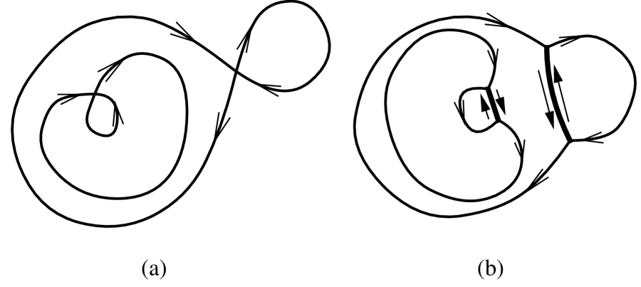
Figure 1: Asymptotic separatrix structures resulting from iso-topological relaxation. Topologically nontrivial initial state (a) leads to the formation of a relaxed state (b) with current sheets (shown bold). The arrows indicate the direction of the magnetic field.

The orientation of the current sheet is such as to lie within a “figure eight” separatrix and to border the outside of an “inside-out figure eight.”

It appears that the final state $a^{\prime}_{\infty}$ of the iso-topological relaxation is uniquely determined by the initial state $a^{\prime}_{0}$. The same is true of the corresponding magnetic fluxes $a_{s}$ and $a_{0}$, once the function ${\gamma}(a)$ [and thereby ${\Gamma}(a)$] is known. Even without any information about ${\gamma}(a)$ the appearance of the relaxed state is well understood qualitatively through the above construct, because applying a function to $a$ does not change the geometry of magnetic field lines.

V.A Comparison with numerical data

The computation of the long-time evolution of nearly ideal 2D MHD turbulence reported by Biskamp and Welter [5] clearly shows current sheets terminating at $Y$ points, which are characteristic of the asymptotic separatrix structures, although the reconnection due to finite magnetic (hyper)diffusivity smears out the individual topology of separatrices.

The spatial distribution of the fluctuations $({\widetilde{a}},{\widetilde{{\psi}}})$ is determined by the eigenfunctions of operator (34). The potential of this operator involves second spatial derivatives of $a_{s}$ (through the term ${\beta}^{*}$). The singularities of $j_{s}=-{\mbox{\boldmath$\bf\nabla$}}^{2}a_{s}$ are delta-function singularities at current sheets. This must lead to the localization of the wavefunctions (the fluctuations) near the potential wells (the current sheets) where ${\gamma}^{\prime\prime}(a_{s}){\mbox{\boldmath$\bf\nabla$}}^{2}{\gamma}(a_{s})<0$. This kind of localization of the microscopic turbulence near the current sheets is indeed observed in the computation of Ref. [5]. Earlier simulations of turbulent magnetic reconnection [50, 51] also confirm this picture.

V.B Iso-topological relaxation and magnetic reconnection

So far we were mostly concerned with the ideal model of two-dimensional MHD, and the question is in order as to the evolution of a more realistic dissipative system involving finite electrical resistivity and fluid viscosity. In general, this is a very difficult problem, because no straightforward perturbation theory can be built for small coefficients appearing in front of higher derivatives in the equations. We therefore restrict ourselves to the qualitative analysis of the role of small dissipation.

If the dissipation is small, the system behavior clearly must resemble, up to a certain point, the prediction of the ideal MHD theory. The deviation of a weakly dissipative evolution from the ideal behavior is always a matter of time of the evolution. In order to neglect the effects of dissipation in MHD turbulence relaxation, not only must the resistivity ${\eta}$ and the viscosity $\nu$ be small but also the length scales should be sufficiently large. The ideal MHD evolution discussed above does lead to the formation of small scale structures which trigger, in the long run, the strong effects of the weak dissipation.

If the initial state is smooth, the small-scale structures do not appear at ones; it takes several nonlinear (eddy turnover) times for the small scales to show up. In the meantime, the system evolves towards, however not quite attains, the ideal statistical equilibrium. In fact, the principal manifestation of approaching the statistical equilibrium is the separation of scales into long-wavelength coherent structures and short-wavelength fluctuations. It is reasonable to assume that this separation of scales is not only necessary, but also sufficient for the statistical equilibrium to set in. Then, by the time when the initially small dissipation becomes important, the coherent part of the turbulent field is essentially built by the statistical mechanics of ideal MHD turbulence. The smaller the dissipation, the shorter scales are allowed to evolve in the Hamiltonian fashion, and therefore the closer the attained shape of the coherent structures to the exact predictions of the Gibbs-ensemble theory.

The time scale ${\tau}^{*}$ specifying the crossover from the ideal regime to the dissipative regime is certainly much shorter than the diffusive time ${\tau}_{\eta}\sim(k_{s}^{2}c^{2}{\eta})^{-1}$ and may not be very long compared to the characteristic nonlinear time ${\tau}_{A}$. Numerical results [6, 9] indicating the enstrophy decay in 2D fluid in just a few eddy turnover times suggest that ${\tau}^{*}/{\tau}_{A}$ is a small power or even logarithm of the large Reynolds number. The fast crossover to the dissipative regime directly indicates the fast production of small scales and, therefore, the equally fast approaching to the statistical equilibrium.

After the approximate equilibrium is set in, the dissipation takes over and the small-scale fluctuations are significantly damped over several times ${\tau}^{*}$, whereas the coherent structures remain little affected, at least in the case when these structures involve no singularities.

If the initial magnetic field has $x$ points, the coherent structure will develop current sheets. The coherent structure will then undergo fast magnetic reconnection. The reconnection occurs in a characteristic time ${\tau}_{r}$ much longer than the Alfvénic time ${\tau}_{A}$, if the magnetic Reynolds number $R_{m}={\tau}_{\eta}/{\tau}_{A}$ is large. By different models, ${\tau}_{r}/{\tau}_{A}$ ranges from $R_{m}^{1/2}$ [52, 53] to $(\ln R_{m})^{p},\ p>0$ [54, 55], although the former (Sweet-Parker) model appears to be more typical [56].

So the ideal MHD turbulence theory describes the early, $t<\min({\tau}^{*},{\tau}_{r})$, iso-topological stage of the turbulent MHD relaxation and predicts the appearance of the coherent structures entering the later stages where magnetic reconnection and/or viscosity play the dominant role. Even then, some topological invariants survive better than others, also providing useful variational tools for the prediction of fully relaxed [57, 58, 59, 60, 61] or selective-decay [6, 9] states.

Our theory can be used to qualitatively describe the relatively early stage, ${\tau}_{A}\ll t\ll({\tau}_{A}{\tau}_{\eta})^{1/2}$, of the nonlinear kink tearing mode in a tokamak, where two dimensional MHD models are commonly used for helically symmetric magnetic perturbations [40, 58, 41, 62]. The kink tearing is accompanied by changes in magnetic topology. First, an $x$ point in the “auxiliary magnetic field” ${\bf B}_{*}={\bf B}-q{\bf B}_{\theta}$ is created near the linearly unstable $q=1$ surface. Then the resulting “magnetic bubble” is pushed to the exterior of the plasma column by essentially ideal MHD motions. This process is likely to be of turbulent nature and, until very small scales are generated, the ideal turbulent relaxation will proceed in the direction of forming a coherent structure with a current sheet corresponding to the initial $x$ point, as suggested by the Gibbs statistics. This stage of evolution may be pretty long, as the magnetic Reynolds number in tokamaks can be of order $10^{6}$ and more. Later on, magnetic reconnection via the current sheet [56] will occur at a characteristic time of order $({\tau}_{A}{\tau}_{\eta})^{1/2}$. Dynamically, the reconnection develops through a sequence of singular MHD equilibria with the same local helicity [58], as analytically described by Waelbroeck [62]. The first of the sequence of these current-sheet equilibria can be interpreted as the asymptotic separatrix structure arising from the initial state via the iso-topological turbulent relaxation.

VI Summary and conclusion

The main result of this paper lies in working out the Gibbs statistics for a Hamiltonian PDE system with an infinity of constants of the motion. This formalism was demonstrated in the example of two dimensional magnetohydrodynamics but can be carried over to other systems. We review again the principal steps of our approach in terms of a general nonlinear Hamiltonian system describing the fields ${\mbox{\boldmath$\bf\psi$}}({\bf x},t)$ and having a finite or an infinite number of invariants ${\bf I}[{\mbox{\boldmath$\bf\psi$}}]=I_{1}[{\mbox{\boldmath$\bf\psi$}}],I_{2}[{\mbox{\boldmath$\bf\psi$}}],\ldots$. Here it does not matter what these invariants are; one can think of $I_{1}$ as the energy and of the rest as topological invariants.

1. The solution to the underlying nonlinear system is sought in the form ${\mbox{\boldmath$\bf\psi$}}({\bf x},t)={\mbox{\boldmath$\bf\psi$}}_{s}({\bf x})+{\widetilde{{\mbox{\boldmath$\bf\psi$}}}}({\bf x},t)$, where ${\mbox{\boldmath$\bf\psi$}}_{s}({\bf x})$ is yet unspecified stationary, Lyapunov stable solution (coherent structure). We then anticipate that the amplitude of the fluctuation field ${\widetilde{{\mbox{\boldmath$\bf\psi$}}}}({\bf x},t)$ is going to be small and hence the exact integrals of motion can be expanded about the coherent structure ${\mbox{\boldmath$\bf\psi$}}_{s}$ up to quadratic terms: ${\bf I}={\bf I}_{s}+{\widetilde{{\bf I}}}$.

2. The Gibbs ensemble is introduced in the fluctuation space in the standard form of the exponential of a linear combination of all invariants, $P[{\widetilde{{\mbox{\boldmath$\bf\psi$}}}}]=\exp(-{\mbox{\boldmath$\bf\alpha$}}\cdot{\widetilde{{\bf I}}})$, where ${\mbox{\boldmath$\bf\alpha$}}={\alpha}_{1},{\alpha}_{2},\ldots$ are the reciprocal temperatures to be determined from the initial state. Having an infinity of Casimirs, which depend on an arbitrary function, is not an obstacle, because any linear combination of the Casimirs is again one of them. In order to have non-diverging fluctuations, we exercise our right to suitably choose the coherent structure ${\mbox{\boldmath$\bf\psi$}}_{s}$. Namely, ${\mbox{\boldmath$\bf\psi$}}_{s}({\bf x})$ is required to minimize the linear combination ${\mbox{\boldmath$\bf\alpha$}}\cdot{\bf I}[{\mbox{\boldmath$\bf\psi$}}]$ of the invariants, where the stationarity of the resulting state is ensured by the Arnold variational principle. Then ${\mbox{\boldmath$\bf\alpha$}}\cdot{\widetilde{{\bf I}}}$ is a positive definite quadratic form, and the Gibbs distribution of the fluctuations is a Gaussian distribution. From now on, the standard Boltzmann-Gibbs statistics is applied in a straightforward way, at least for a finite dimensional approximation using $N$ eigenmode amplitudes $f_{m}$ satisfying the Liouville theorem.

3. The eigenmodes are introduced such as to diagonalize the Gibbs exponential, ${\mbox{\boldmath$\bf\alpha$}}\cdot{\widetilde{{\bf I}}}=({\alpha}_{1}/2)\sum_{m}{\lambda}_{m}f_{m}^{2}$. Then averages can be computed in the conservation laws, ${\bf I}_{0}={\bf I}_{s}+\left<{\widetilde{{\bf I}}}[{\widetilde{{\mbox{\boldmath$\bf\psi$}}}}]\right>$, in order to infer the equations for the temperatures.

4. The fluctuations’ share of the invariants, $\left<{\widetilde{{\bf I}}}[{\widetilde{{\mbox{\boldmath$\bf\psi$}}}}]\right>=\sum_{m}1/(2{\alpha}_{1}{\lambda}_{m}){\partial}^{2}{\widetilde{{\bf I}}}/{\partial}f_{m}^{2}$, when expanded in the eigenmodes, turns out to diverge as $N\to\infty$, unless the temperatures $1/{\alpha}_{m}$ are let to zero (even then the temperature ratios remain finite and keep useful information). This is the “ultraviolet catastrophe.” The regularization of this divergence requires the reciprocal temperatures to also diverge, e.g., ${\alpha}_{1}(N)\propto N$.

5. If the square norm of the fluctuations $\left<{\widetilde{{\mbox{\boldmath$\bf\psi$}}}}|{\widetilde{{\mbox{\boldmath$\bf\psi$}}}}\right>=\sum_{m}({\alpha}_{1}{\lambda}_{m})^{-1}$ diverges at constant temperatures slower (e.g., logarithmically) than the fastest diverging invariant (say, the energy $I_{1}$), then the average norm goes to zero as $N\to\infty$. This is the crucial point, which justifies the assumption of the small amplitude necessary for the Gaussianity of the fluctuations in the given representation. If this condition is not fulfilled, one can always pick other variables involving lower order of derivatives, such as ${\mbox{\boldmath$\bf\psi$}}^{\prime}={\mbox{\boldmath$\bf\nabla$}}^{-2}{\mbox{\boldmath$\bf\psi$}}$, and repeat the above steps. However, the exact Gaussianity of the fluctuations requires another important property of the integrals of motion, which is independent of the variables used. Namely, each invariant must be not more than quadratic in the highest-order-derivative variables. Then the quadratic expansion will be also valid even for those (fastest diverging) invariants, whose fluctuations are finite. This property holds for 2D MHD, but it does not for 2D Euler turbulence or Vlasov-Poisson system (Appendix D).

6. If, in addition, there are invariants (such as magnetic topology invariants) diverging slower than the fastest diverging integral of motion, then the average fluctuation’s share of those invariants vanishes as $N\to\infty$. The presence of such invariants simplifies the analysis of the coherent structure.

We use the above steps to study the relaxation of ideal two dimensional MHD turbulence, where both infinite sets of topological invariants, magnetic (6) and cross (7), are incorporated. We show that accounting for all topological invariants leads to the prediction that the long evolved MHD turbulent state consist of a coherent structure (the most probable state) and a small-amplitude, small-scale Gaussian turbulence (the fluctuations). The fluctuations are small if measured in terms of the magnetic vector potential ${\widetilde{a}}$ and the flow stream function ${\widetilde{{\psi}}}$. The fluctuations in the magnetic field ${\widetilde{{\bf B}}}$ and the fluid velocity ${\widetilde{{\bf v}}}$ are of the same order as in the coherent structure. The fluctuation current ${\widetilde{{\bf j}}}$ and vorticity ${\widetilde{{\omega}}}$ are infinite in the long time limit.

We find that in 2D ideal MHD turbulence the coherent structure has the same magnetic topology as the initial state, while energy and cross topology are shared between the coherent structure and the fluctuations. Therefore, for a sufficiently wide class of initial conditions having the same topological invariants, the final coherent state is the same, whereas the fluctuations, when measured by the standard norm (54), become asymptotically “invisible.” In this sense, the coherent structures emerging from the turbulent MHD relaxation can be regarded as “topological attractors,” even though the underlying dynamics is perfectly Hamiltonian. (The theorem of the absence of attractors in Hamiltonian systems is not valid for infinite dimensional PDE systems.)

The presence of the fluctuations on the top of the coherent structure is conceptually important even though the amplitude of these fluctuations goes to zero in the long time limit: the fluctuations appear as the storage of the “lost” integrals of motion, if only the most probable state is compared with the initial state. This explains the well-known result (cf. [23]), that the topological invariants of the coherent vortex emerging from 2D Euler turbulence, are different from those of the initial state. In 2D magnetohydrodynamics the role of the initial topology is more important. In Appendix D we discuss the application of the Gibbs-ensemble formalism to the two dimensional Euler equation.

We formulate the variational principle of iso-topological relaxation, which allows us to predict the shape of the coherent structure for the given initial state. We show how the problem of the ideal MHD relaxation with plasma flow is reduced to the viscous relaxation of magnetic field with no flow in the final state. The numerical results suggest that the asymptotic separatrix structures with current sheets are indeed observed during the turbulent relaxation. It appears that these structures are the route to reconnection in the nonlinear kink tearing mode in tokamaks.

Many problems of MHD turbulence remain, most notably the role of small dissipation. As discussed in Sec. V.B, this is the dynamics of producing small scales which determines when and how the dissipative processes become important. In order to study the phenomena of crossover from the ideal to the dissipative turbulent relaxation, the nonequilibrium dynamics of the ideal relaxation must be worked out. It appears that the formalism of the weak turbulence theory [15, 63, 64] can be appropriately suited for Eq. (B.1) in order to study the nonequilibrium statistics of 2D MHD turbulence. However, the important role of the ideal Gibbs turbulence for weakly dissipative systems is found in that the ideal turbulence forms predictable coherent structures, which enter the later, dissipative stages of the turbulent evolution.

The comparison of the MHD and the Euler turbulence prompts us to distinguish between three kinds of advected fields. The first kind is passive field, such as the concentration of a dye or the temperature that do not affect the advecting velocity field. Passive fields tend to become spatially uniform due to turbulent diffusion. The second kind is active field, such as the vorticity in Euler fluid, which does affect the velocity field but whose lines or contours can be indefinitely stretched at no significant energy price. The active fields therefore tend to self-organize assuming topologically simple structures, like monopole vortices, whose topology is different from that of the initial state. The third kind can be referred to as “reactive field,” such as the magnetic flux frozen into an ideally conducting fluid. Stretching of magnetic field lines is energetically expensive and cannot last indefinitely. The topology of the reactive field is therefore much more robust than that of passive or active fields, and the self-organization can lead to nontrivial coherent structures with singularities (current sheets).

Acknowledgments

We wish to thank V. V. Yankov, P. J. Morrison, F. L. Waelbroeck, F. Porcelli, P. H. Diamond, G. E. Falkovich, and J. B. Taylor for stimulating discussions. This work was partially supported by the U.S. Department of Energy under Contracts No. DE-FGO3-88ER53275 and DE-FG05-80ET53088.

APPENDICES

Appendix A Extremal properties and stability of MHD and Euler equilibria: Positive and negative temperatures

Lyapunov stability of equilibria in conservative systems depends on the extremal properties of their invariants. The strongest form of the relevant Lyapunov theorem states that if a state realizes a conditional nondegenerate extremum (that is, a minimum or a maximum) of one of the invariants subject to the conservation of one or more of other invariants, then this state is stable. It is emphasized that the above is the sufficient criterion for nonlinear stability with respect to any sufficiently small perturbations. Originally formulated for finite dimensional systems, the Lyapunov theorem is extended to PDE systems on a case-by-case basis and depends on the functional norm used to specify what “small” means [65].

The existence of such extremal, and therefore stable, states can be detected by inspecting various inequalities involving integrals of motion. As an example, consider 2D MHD states with the fixed cross helicity (8),

$$\int{\mbox{\boldmath$\bf\nabla$}}a\cdot{\mbox{\boldmath$\bf\nabla$}}{\psi}\,d^{2}{\bf x}=J_{1}\ .$$ (A.1)

Then the energy (3) is clearly bounded from below,

$$E\geq|J_{1}|\ ,$$ (A.2)

which indicates the existence of a minimum-energy state subject to the conservation of the topological invariants. An example of such a state is any circular magnetic configuration $a=a(r)$ with no fluid flow, ${\psi}=0$. This configuration assumes the absolute minimum of energy with respect to all neighboring iso-topological MHD states. Indeed, the magnetic force is the tension of magnetic field lines, which tend to shrink while preserving the area inside them. The smallest perimeter at fixed area is assumed by a circle.

A formal proof, which can be extended to more interesting geometries, can be given in terms of the iso-topological energy variation (15)—(16). The first variation is vanishing at an equilibrium state, and the second is given by the general form

$${\delta}^{2}E_{m} = \int\left[-\{\mu,a\}\{\mu,j\}+\left({\mbox{\boldmath$\bf\nabla$}}\{\mu,a\}\right)^{2}\right]d^{2}{\bf x}\ ,$$ (A.3)

$${\delta}^{2}E_{f} = \int\left[({\mbox{\boldmath$\bf\nabla$}}{\delta}{\psi})^{2}-\{\mu,{\psi}\}\{\mu,{\omega}\}-\{\mu,{\psi}\}\{\nu,a\}-\{\mu,a\}\{\nu,{\psi}\}\right]d^{2}{\bf x}\ ,$$ (A.4)

for the magnetic and the fluid kinetic energy, respectively.

Upon letting $a=a(r)$ and Fourier expanding the azimuthal-angle-periodic displacement function $\mu(r,{\theta})=\sum\mu_{m}(r)\exp(im{\theta})$, several integrations by parts (presuming that $\mu$ goes to zero sufficiently fast for both $r\to 0$ and $r\to\infty$) yield

$${\delta}^{2}E_{m}=\sum_{m=-\infty}^{\infty}m^{2}\int_{0}^{\infty}\frac{dr}{r^{3}}\left(\frac{da}{dr}\right)^{2}\left(m^{2}|\mu_{m}(r)|^{2}+|\mu_{m}(r)-r\mu_{m}^{\prime}(r)|^{2}\right)>0\ .$$ (A.5)

Equation (A.4) also implies ${\delta}^{2}E_{f}>0$ for ${\psi}=0$. That is, any circular magnetic field without fluid flow assumes the conditional minimum of energy subject to the conservation of topological invariants and is therefore Lyapunov stable. Adding a small fluid velocity along the circular magnetic field lines will not change the stability of such an equilibrium.

It is easy to see that there is no upper bound on the MHD energy, even though all the topological invariants (6)-(7) are fixed: by an incompressible convolution of the magnetic field lines the magnetic energy can be made arbitrarily large.

The kinetic fluid energy can be represented in the form of “electrostatic” energy of charges with the density ${\omega}$,

$$E_{f}=\frac{1}{2}\int{\psi}{\omega}\,d^{2}{\bf x}=\frac{1}{2}\int{\omega}({\bf x}_{1}){\omega}({\bf x}_{2})G({\bf x}_{1},{\bf x}_{2})\,d^{2}{\bf x}_{1}d^{2}{\bf x}_{2}\ ,$$ (A.6)

where the Green function $G$  [$=-(1/2\pi)\ln|{\bf x}_{1}-{\bf x}_{2}|$ for an infinite domain] plays the role of the interaction potential. The total charge, $J_{0}=\int{\omega}d^{2}{\bf x}$, is conserved, and the charges are allowed to redistribute only along the magnetic field lines [in MHD: invariants (7)] or by means of incompressible interchanges [in Euler equation: integrals (D.3)].

The extremal properties of two dimensional Euler fluid are different from those of MHD in that the energy has also an upper bound at fixed topological invariants. According to the Schwarz inequality, we have

$$E_{f}^{2}\leq\frac{1}{4}\int{\omega}^{2}({\bf x}_{1}){\omega}^{2}({\bf x}_{2})\,d^{2}{\bf x}_{1}d^{2}{\bf x}_{2}\int G^{2}({\bf x}_{1},{\bf x}_{2})\,d^{2}{\bf x}_{1}d^{2}{\bf x}_{2}={\rm const}\,I_{2}^{2}\ ,$$ (A.7)

where $I_{2}=\int{\omega}^{2}d^{2}{\bf x}$ is the conserved fluid enstrophy, and we have used the quadratic integrability of the Green function, which has only logarithmic singularity at ${\bf x}_{1}={\bf x}_{2}$. By collecting the most intensive charges closest to each other—that is, forming a circular vortex with a monotonically decreasing vorticity of the same sign, we construct the maximum-energy state [33]. Such vortices play an important role in 2D Euler turbulence [7]. Conversely, a monotonically increasing vorticity in a circular domain assumes the minimum of energy under fixed topological invariants.

Adding even a small amount of magnetic field to the maximum-energy stable vortices will drive them unstable, because the negative-energy waves perturbing the vortices will dump their energy into the magnetic field via magnetic dynamo and thereby grow in amplitude. The resulting turbulent relaxation will lead to other, minimum-energy equilibria, which may be non-circular due to the competition of the elastic tension of magnetic field lines with the repulsion of the “vorticity charges” threaded onto these lines.

As discussed in Sec. IV.C, the Gibbs distribution of fluctuations about an equilibrium coherent structure has the form of

$$\exp[-{\alpha}{\delta}^{2}(E+{\rm Topological\ Invariants})/2]\ ,$$ (A.8)

where ${\alpha}=1/T_{E}$ is the reciprocal temperature conjugate to energy and ${\delta}^{2}$ the second (unconstrained) variation specifying the fluctuations. In order for the fluctuations to be finite, the temperature must be positive for minimum-energy states, as it is in ordinary world or in 2D MHD, and negative for maximum-energy states, as is possible in 2D ideal fluid [1, 27, 28]

Appendix B Liouvillianity of dynamical variables

The probability distribution functional (38) is meant to describe the statistical properties of the fluctuations. The dynamics governing the amplitudes $f_{m}(t)$ can be written by substituting the eigenmode decomposition (32) into Eqs. (1) and (2). Then, using the orthonormal properties of the eigenmodes, we obtain

$$\dot{f}_{m}=\sum_{n}H_{mn}f_{n}+\sum_{np}H_{mnp}f_{n}f_{p}\ ,$$ (B.1)

where

$$H_{mn} = \int[a_{m}\{{\psi}_{n},a_{s}\}+a_{m}\{{\psi}_{s},a_{n}\}+$$

$${\omega}_{m}\{{\psi}_{n},{\omega}_{s}\}+{\omega}_{m}\{{\psi}_{s},{\omega}_{n}\}+{\omega}_{m}\{j_{n},a_{s}\}+{\omega}_{m}\{j_{s},a_{n}\}]d^{2}{\bf x}\ ,$$ (B.2)

$$H_{mnp} = \int\left[a_{m}\{{\psi}_{n},a_{p}\}+{\omega}_{m}\{{\psi}_{n},{\omega}_{p}\}+{\omega}_{m}\{j_{n},a_{p}\}\right]d^{2}{\bf x}\ ,$$ (B.3)

the indices $m,n$, and $p$ refer to the eigenmodes and $s$ to the coherent structure. The divergence of the phase-space flow defined by Eq. (B.1),

$$\sum_{m}{\partial}\dot{f}_{m}/{\partial}f_{m}=\sum_{m}H_{mm}+\sum_{mn}(H_{mmn}+H_{mnm})f_{n}\ ,$$ (B.4)

must be zero for Liouvillian variables. This is generally not true even for the first term on the RHS of Eq. (B.4). However, a linear change to new variables can kill the zero-order term in Eq. (B.4). An example of new variables is given by the eigenmode amplitudes of another linear operator,

$$W^{\prime}\left(\begin{array}[]{l}{\widetilde{a}}\\ {\widetilde{{\omega}}}\end{array}\right)=\left(\begin{array}[]{ll}({\beta}^{*}-{\mbox{\boldmath$\bf\nabla$}}^{2})&\quad{\gamma}^{\prime}\\ {\gamma}^{\prime}&-{\mbox{\boldmath$\bf\nabla$}}^{-2}\end{array}\right)\left(\begin{array}[]{l}{\widetilde{a}}\\ {\widetilde{{\omega}}}\end{array}\right)\equiv\left(\begin{array}[]{c}{\beta}^{*}{\widetilde{a}}+{\widetilde{j}}+{\gamma}^{\prime}{\widetilde{{\omega}}}\\ {\gamma}^{\prime}{\widetilde{a}}+{\widetilde{{\psi}}}\end{array}\right)\ ,$$ (B.5)

such that the fluctuation part of $E+I_{\beta}+J_{\gamma}$ can be formally written as

$$\left<\begin{array}[]{l|}{\widetilde{a}}\\ {\widetilde{{\omega}}}\end{array}\right.W^{\prime}\left.\begin{array}[]{|l}{\widetilde{a}}\\ {\widetilde{{\omega}}}\end{array}\right>\ .$$ (B.6)

Then, in terms of the new eigenmodes, the equation of motion can be written exactly as Eqs. (B.1), (B.2), and (B.3); however, the equations for the eigenfunctions $a_{m}$ and ${\omega}_{m}$ are different from those of the old operator $W$ (34). The usefulness of the new variables is that the zero-order term $H_{mm}$ in Eq. (B.4) identically vanishes after integrating by parts for each $m$, whereas the linear term,

$$H_{mmn}+H_{mnm}=\int\left[{\gamma}^{\prime}\{(a_{m}^{2}+{\omega}_{m}^{2})/2,a_{n}\}+{\gamma}^{\prime}\{{\omega}_{m},a_{m}{\omega}_{n}\}+{\beta}^{*}\{{\omega}_{m},a_{m}a_{n}\}\right]d^{2}{\bf x}\ ,$$ (B.7)

generally persists unless there is no inhomogeneity due to the coherent structure. Nevertheless, the remaining linear term in Eq. (B.4) vanishes as the amplitude goes to zero. Thus the new variables $f_{m}$ are Liouvillian only in the limit of vanishing amplitudes, which is also the assumption lying behind the Gaussian distribution (38). The validity of this assumption is confirmed in Sec. IV.D.

As the change from the old to the new variables is a linear transformation, the non-Liouvillianity of the old variables only leads to a constant weighting factor—the Jacobian—in the probability (38), which does not affect the averaging. Hence we may write $\prod_{m}df_{m}$ in the functional integrals in (22) instead of ${\cal D}a{\cal D}{\psi}$.

Appendix C The spectrum of the eigenmodes

The eigenmode equation for the operator (34) can be written

$$({\lambda}_{m}-{\beta}^{*}+{\mbox{\boldmath$\bf\nabla$}}^{2})a_{m} = -{\gamma}^{\prime}{\mbox{\boldmath$\bf\nabla$}}^{2}{\psi}_{m}\ ,$$ (C.1)

$$\left[-{\gamma}^{\prime}{\mbox{\boldmath$\bf\nabla$}}^{2}-2{\mbox{\boldmath$\bf\nabla$}}{\gamma}^{\prime}{\mbox{\boldmath$\bf\nabla$}}-({\mbox{\boldmath$\bf\nabla$}}^{2}{\gamma}^{\prime})\right]a_{m} = ({\lambda}_{m}+{\mbox{\boldmath$\bf\nabla$}}^{2}){\psi}_{m}\ .$$ (C.2)

We are interested in the high-mode (WKB) limit $m\to\infty$, where we can replace $\bf\nabla$ acting on $a_{m}$ and ${\psi}_{m}$ by $i{\bf k}$. Then we get the quadratic equation for the eigenvalues,

$${\lambda}_{m}^{2}-(2{\bf k}^{2}+{\beta}^{*}){\lambda}_{m}+{\bf k}^{4}(1-{\gamma}^{\prime 2})+i{\bf k}^{2}{\bf k}\cdot{\mbox{\boldmath$\bf\nabla$}}{\gamma}^{\prime 2}+{\bf k}^{2}({\beta}^{*}+{\gamma}^{\prime}{\mbox{\boldmath$\bf\nabla$}}^{2}{\gamma}^{\prime})=0\ ,$$ (C.3)

having the solutions

$${\lambda}^{\pm}_{m}={\bf k}^{2}(1\pm{\gamma}^{\prime})+\frac{{\beta}^{*}}{2}\mp\frac{i{\bf k}\cdot{\mbox{\boldmath$\bf\nabla$}}{\gamma}^{\prime}}{{\gamma}^{\prime}{\bf k}^{2}}+{\cal O}(k^{-2})\ .$$ (C.4)

The corresponding eigenfunctions satisfy

$$\frac{{\psi}_{m}}{a_{m}}=\frac{{\lambda}_{m}-{\bf k}^{2}-{\beta}^{*}}{{\gamma}^{\prime}{\bf k}^{2}}=\pm 1-\frac{{\beta}^{*}}{2{\gamma}^{\prime}{\bf k}^{2}}+{\cal O}(k^{-3})\ .$$ (C.5)

The ordering of the modes with number can be figured out by substituting the zero-order eigenfunction ratio (C.5) into Eq. (C.1):

$$\left(\frac{{\beta}^{*}}{1\pm{\gamma}^{\prime}}-{\mbox{\boldmath$\bf\nabla$}}^{2}\right)a_{m}=\frac{{\lambda}_{m}}{1\pm{\gamma}^{\prime}}a\ .$$ (C.6)

If ${\gamma}^{\prime}$ were constant, Eq. (C.6) would be a standard Schrödinger equation with the Bohr-Sommerfeld quasiclassical energy levels ${\lambda}_{m}^{\pm}=(1\pm{\gamma}^{\prime})4\pi m/{\cal S}$ and the wavenumber (43). In the case of inhomogeneous ${\gamma}^{\prime}$ we arrive at formulas (40) and (41).

Appendix D Gibbs statistics of two dimensional Euler turbulence

Although the Euler equation,

$${\partial}_{t}{\omega}=\{{\psi},{\omega}\}\ ,\quad{\omega}\equiv-{\mbox{\boldmath$\bf\nabla$}}^{2}{\psi}\ ,$$ (D.1)

is a special case of the MHD system (1)-(2) at zero magnetic field, the properties of two dimensional Euler turbulence are drastically different from those of 2D MHD turbulence. This is primarily due to the different structure of the integrals of motion, which for the Euler fluid are energy

$$E=\frac{1}{2}\int({\mbox{\boldmath$\bf\nabla$}}{\psi})^{2}\,d^{2}{\bf x}\ ,$$ (D.2)

and vorticity topology invariants

$$I_{F}=\int F({\omega})\,d^{2}{\bf x}\ .$$ (D.3)

The formal Gibbs ensemble

$$P[{\psi}]=\exp[-{\alpha}(E+I_{\beta})]\simeq P[{\psi}_{s}]\exp\left(-\frac{{\alpha}}{2}\left<{\widetilde{{\psi}}}|W|{\widetilde{{\psi}}}\right>\right)$$ (D.4)

can be approximately written in terms of the eigenmodes of the self-adjoint operator

$$W=-{\mbox{\boldmath$\bf\nabla$}}^{2}+{\mbox{\boldmath$\bf\nabla$}}^{2}{\beta}^{\prime\prime}({\psi}_{s}){\mbox{\boldmath$\bf\nabla$}}^{2}\ ,$$ (D.5)

whose quasiclassical eigenvalues behave as

$${\lambda}_{\bf k}\simeq{\beta}^{\prime\prime}{\bf k}^{4}\ ,\quad{\bf k}_{m}^{2}\simeq\frac{4\pi m}{{\cal S}}\ ,\quad m\gg k_{s}^{2}{\cal S}.$$ (D.6)

Then the fluctuation energy,

$$\left<{\widetilde{E}}\right>\simeq\sum_{m}\frac{1}{2{\alpha}{\lambda}_{m}}\int({\mbox{\boldmath$\bf\nabla$}}{\widetilde{{\psi}}}_{m})^{2}\,d^{2}{\bf x}\sim\sum_{m}\frac{{\bf k}_{m}^{2}}{{\alpha}{\lambda}_{{\bf k}_{m}}}\ ,$$ (D.7)

diverges with the number of modes logarithmically, whereas the topological invariants,

$$\left<{\widetilde{I}}_{F}\right>\simeq\sum_{m}\frac{1}{2{\alpha}{\lambda}_{m}}\int F^{\prime\prime}({\omega}_{s})({\mbox{\boldmath$\bf\nabla$}}^{2}{\widetilde{{\psi}}}_{m})^{2}\,d^{2}{\bf x}\sim\sum_{m}\frac{{\bf k}_{m}^{4}}{{\alpha}{\lambda}_{{\bf k}_{m}}}\ ,$$ (D.8)

diverge linearly with $N$. In this sense, we have something like the equipartition of topology, rather than of energy, between the fluctuation eigenmodes. The square norm of the fluctuation stream function, $\int{\widetilde{{\psi}}}^{2}d^{2}{\bf x}$, converges.

In accordance with the principles (a)—(f) set forth in Sec. VI, we conclude that in the long time limit the fluctuations in the stream function ${\widetilde{{\psi}}}\to 0$. The fluctuation energy (and hence the velocity ${\widetilde{{\bf v}}}$) also goes to zero, but a finite share of the topological invariants gets into the fluctuations.

Hence the coherent structure emerging from 2D Euler turbulence has the same energy, but different vorticity topology, as compared to the initial condition. This state of affairs makes it hard to predict the appearance of the coherent structure from only the analysis of the integrals of motion and requires dynamical considerations.

The real difficulty, however, is that the highest-order-derivative variable, the vorticity ${\omega}$, enters the topological invariants (D.3) in all powers, not only quadratically. This makes the expansion of the topological invariants (D.3) about the coherent structure inaccurate, and hence the Euler turbulence non-Gaussian. As a result, the formally written Gibbs distribution (D.4) is useless for making quantitative predictions, because, as mentioned earlier, non-Wienerian probability functionals do not allow well-defined averages. This difficulty is present even if the validity of the Gibbs ensemble (D.4) is not questioned. We note, however, that this also remains unclear whether or not it is possible to derive the standard canonical ensemble from the first principles set forth in the microcanonical ensemble for the case of non-additive integrals of motion (see also discussion in Sec. IV.A). Thus the “exact” predictions based on the Gibbs statistics of 2D Euler turbulence [23, 24, 25] appear questionable, because the result depends on the discretization used to solve functional integrals, or, equivalently, on the relative size of the “micro-cells” used for a combinatorial treatment. One example of such a dependence is given by the discretization by means of point vortices, where the equilibrium state depends on the (arbitrary chosen) vortex strengths. Another example, dealing with continuum fields, was provided by Lynden-Bell [22] in the context of the Vlasov-Poisson model of a stellar system, where the equilibrium is given by a combination of Maxwell exponentials depending on the arbitrary partitioning of the phase space into micro-cells. There, the source of the ambiguity is the same as in the Euler equation: the highest-order-derivative variable—the star distribution function $f({\bf x},{\bf v},t)$—enters the Casimirs $I_{F}[f]=\int F(f)d{\bf x}d{\bf v}$ not only quadratically.

The non-Gaussianity of 2D Euler turbulence suggests that the Boltzmann-Gibbs formula (D.4) is not valid for such a system. Nevertheless, this does not affect the general trend of splitting into a stationary coherent structure and a small-scale, small-amplitude (in appropriate variables) fluctuations. The dynamics of such an evolution can be also described in terms of structures. If the initial state has the length scale much less than the box size, the coherent part of the turbulence evolves through weakly interacting nearly circular vortices, whose number decreases with time due to the vortex merger [7, 8, 66].

References

- [1] L. Onsager, “Statistical hydrodynamics,” Nuovo Cimento Suppl., vol. 6, p. 279, 1949.
- [2] R. H. Kraichnan and D. Montgomery, “Two-dimensional turbulence,” Rep. Prog. Phys., vol. 43, p. 547, 1980.
- [3] G. A. Kuzmin, “Statistical mechanics of vorticity in a 2D coherent structure,” in Structural turbulence, pp. 103—115, Novosibirsk: Thermophysics Institute, Siberian Branch, Academy of Sciences of the USSR, 1982. In Russian.
- [4] A. M. Polyakov, “The theory of turbulence in two dimensions,” Preprint PUPT-1369, Physics Dept., Princeton University, Princeton, December 1992. Nucl Phys. B?
- [5] D. Biskamp and H. Welter, “Dynamics of decaying two-dimensional magnetohydrodynamic turbulence,” Phys. Fluids, vol. B 1, p. 1964, 1989.
- [6] W. H. Matthaeus, W. T. Stribling, D. Martinez, S. Oughton, and D. Montgomery, “Selective decay and coherent vortices in two-dimensional incompressible turbulence,” Phys. Rev. Lett., vol. 66, no. 21, pp. 2731—2734, 1991.
- [7] G. F. Carnevale, J. C. McWilliams, Y. Pomeau, J. B. Weiss, and W. R. Young, “Evolution of vortex statistics in two-dimensional turbulence,” Phys. Rev. Lett., vol. 66, no. 21, pp. 2735—2737, 1991.
- [8] G. F. Carnevale, J. C. McWilliams, Y. Pomeau, J. B. Weiss, and W. R. Young, “Rates, pathways, and end states of nonlinear evolution in decaying two-dimensional turbulence: Scaling theory versus selective decay,” Phys. Fluids, vol. A 4, no. 6, pp. 1314—1316, 1991.
- [9] D. Montgomery, W. H. Matthaeus, W. T. Stribling, D. Martinez, and S. Oughton, “Relaxation in two dimensions and the “sinh-Poisson” equation,” Phys. Fluids, vol. A 4, no. 1, pp. 3—6, 1992.
- [10] H. Tasso, “Equilibrium statistics of some evolution equations,” Phys. Lett., vol. A 120, no. 9, pp. 464—465, 1987.
- [11] J. L. Lebowitz, H. A. Rose, and E. R. Speer, “Statistical mechanics of the nonlinear Schrödinger equation,” J. Stat. Phys., vol. 50, no. 3/4, pp. 657—686, 1988.
- [12] J. L. Lebowitz, H. A. Rose, and E. R. Speer, “Statistical mechanics of the nonlinear Schrödinger equation. II. Mean field approximation,” J. Stat. Phys., vol. 54, no. 1/2, pp. 17—56, 1989.
- [13] Y. Pomeau, “Long time behavior of solutions of nonlinear classical field equations: the example of NLS defocusing,” Physica, vol. D 61, pp. 227—239, 1992.
- [14] T. D. Lee Quart. Appl. Math., vol. 10, p. 69, 1952.
- [15] G. E. Falkovich and A. Shafarenko, “Nonstationary wave turbulence,” J. Nonlinear Science, vol. 1, pp. 457—480, 1991.
- [16] V. E. Zakharov, “Collapse of Langmuir waves,” Zh. Eksp. Teor. Fiz., vol. 62, p. 1745, 1972. [English transl. Sov. Phys. JETP 35, 908—914 (1972)].
- [17] V. Zeitlin, “Finite-mode analogs of 2D ideal hydrodynamics: Coadjoint orbits and local canonical structure,” Physica, vol. D 49, pp. 353—362, 1991.
- [18] R. H. Kraichnan, “Inertial ranges in two-dimensional turbulence,” Phys. Fluids, vol. 10, no. 7, pp. 1417—1423, 1967.
- [19] R. H. Kraichnan J. Fluid Mech., vol. 67, p. 155, 1975.
- [20] D. Fyfe and D. Montgomery, “High-beta turbulence in two-dimensional magnetohydrodynamics,” J. Plasma Phys., vol. 16, no. 2, pp. 181—191, 1976.
- [21] J. F. Carnevale and J. S. Frederiksen, “Nonlinear stability and statistical mechanics of flow over topography,” J. Fluid Mech., vol. 175, pp. 157—181, 1987.
- [22] D. Lynden-Bell, “Statistical mechanics of violent relaxation in stellar systems,” Mon. Not. R. Astr. Soc., vol. 136, pp. 101—121, 1967.
- [23] J. Miller, “Statistical mechanics of Euler equation in two dimensions,” Phys. Rev. Lett., vol. 65, no. 17, pp. 2137—2140, 1990.
- [24] R. Robert and J. Sommeria, “Statistical equilibrium states for two-dimensional flows,” J. Fluid Mech., vol. 229, pp. 291—310, 1991.
- [25] J. Miller, P. Weichman, and M. Cross, “Statistical mechanics, Euler’s equation, and Jupiter’s Red Spot,” Phys. Rev., vol. A 45, no. 4, pp. 2328—2359, 1992.
- [26] M. B. Isichenko, “Can computer simulation predict the real behavior of turbulence?,” Comments on Plasma Phys. Controlled Fusion, vol. 16, no. 3, pp. 187—206, 1995.
- [27] D. Montgomery and G. Joyce, “Statistical mechanics of “negative temperature states”,” Phys. Fluids, vol. 17, no. 6, p. 1139, 1973.
- [28] S. F. Edwards and J. B. Taylor, “Negative temperature states of two-dimensional plasmas and vortex fluids,” Proc. R. Soc. Lond., vol. A 336, pp. 257—271, 1974.
- [29] J. Fröhlich and D. Ruelle, “Statistical mechanics of vortices in an inviscid two-dimensional fluid,” Commun. Math. Phys., vol. 87, pp. 1—36, 1982.
- [30] V. Berdichevsky, I. Kunin, and F. Hussain, “Negative temperature for vortex motion,” Phys. Rev., vol. A 43, no. 4, p. 2050, 1991.
- [31] D. Biskamp and U. Bremer, “Dynamics and statistics of inverse cascade processes in 2D magnetohydrodynamic turbulence,” Phys. Rev. Lett., vol. 72, no. 24, p. 3819, 1994.
- [32] S. F. Krylov and V. V. Yankov, “On the role of solitons in strong turbulence,” Zh. Eksp. Teor. Fiz., vol. 79, p. 82, 1980. [English transl. Sov. Phys. JETP 52, 41 (1980)].
- [33] V. I. Petviashvili and V. V. Yankov, “Solitons and turbulence,” in Reviews of Plasma Physics (B. B. Kadomtsev, ed.), vol. 14, p. 1, New York: Consultants Bureau, 1989.
- [34] A. I. Dyachenko, V. E. Zakharov, A. N. Pushkarev, V. F. Shvets, and V. V. Yankov, “Soliton turbulence in nonintegrable systems,” Zh. Eksp. Teor. Fiz., vol. 96, pp. 2026—2031, 1989. [English transl. Sov. Phys. JETP 69(6), 1144—1147 (1989)].
- [35] A. V. Gruzinov, “Gaussian free turbulence,” Zh. Eksp. Teor. Fiz., vol. 103, pp. 467—475, 1993. [English transl. JETP 76(2), 241—244 (1993)].
- [36] P. J. Morrison and R. D. Hazeltine, “Hamilton formulation of reduced magnetohydrodynamics,” Phys. Fluids, vol. 27, p. 886, 1984.
- [37] M. B. Isichenko and A. M. Marnachev, “Nonlinear wave solutions of electron MHD in a uniform plasma,” Zh. Eksp. Teor. Fiz., vol. 93, pp. 1244–1255, 1987. [Sov. Phys. JETP 66(4), 702—708 (1987)].
- [38] A. V. Gruzinov, “Gaussian free turbulence: structures and relaxation in plasma models,” Plasma Phys. Controlled Fusion, vol. 15, p. 227, 1993.
- [39] A. C. Ting, W. H. Matthaeus, and D. Montgomery, “Turbulent relaxation processes in magnetohydrodynamics,” Phys. Fluids, vol. 29, p. 3261, 1986.
- [40] B. B. Kadomtsev and O. P. Pogutse, “Nonlinear helical plasma perturbations in the tokamak,” Zh. Eksp. Teor. Fiz., vol. 65, pp. 575—589, 1973. [English transl. Sov. Phys. JETP 38, 283 (1973)].
- [41] M. N. Rosenbluth, D. A. Monticello, H. R. Strauss, and R. B. White, “Numerical studies of nonlinear evolution of kink modes in tokamaks,” Phys. Fluids, vol. 19, p. 198, 1976.
- [42] H. R. Strauss, “Nonlinear, three-dimensional magnetohydrodynamics of noncircular tokamaks,” Phys. Fluids, vol. 19, p. 134, 1976.
- [43] Y. G. Sinai, “Dynamical systems with elastic reflections,” Russ. Math. Survey, vol. 25, p. 137, 1970.
- [44] M. B. Isichenko, “Percolation, statistical topography, and transport in random media,” Rev. Mod. Phys., vol. 64, no. 4, pp. 961—1043, 1992.
- [45] N. Wiener, Nonlinear problems in random theory. New York: Wilely, 1958.
- [46] R. P. Feynman and A. R. Hibbs, Quantum mechanics and path integrals. New York: McGraw-Hill, 1965.
- [47] S. I. Syrovatskii, “Formation of current sheets in a plasma with a frozen-in strong magnetic field,” Zh. Eksp. Teor. Fiz., vol. 60, no. 5, pp. 1727—1741, 1971. [English transl. Sov. Phys. JETP 33(5), 933 (1971)].
- [48] V. I. Arnold, “The asymptotic Hopf invariant and its applications,” in Proceedings of the All-Union Summer School on Partial Differential Equations (Dilizhan, Armenia, 1974), (Erevan), p. 229, Armenian SSR Academy of Sciences Press, 1974. [English transl. Sel. Math. Sov. 5, 327—345 (1986)].
- [49] H. K. Moffatt, “Structure and stability of solutions of the Euler equation: a lagrangian approach,” Phil. Trans. R. Soc. Lond., vol. A 333, pp. 321—342, 1990.
- [50] W. H. Matthaeus and S. L. Lamkin, “Turbulent magnetic reconnection,” Phys. Fluids, vol. 29, no. 8, pp. 2513—2534, 1986.
- [51] W. H. Matthaeus and D. Montgomery, “Nonlinear evolution of the sheet pinch,” J. Plasma Phys., vol. 25, no. 1, pp. 11—41, 1981.
- [52] P. A. Sweet, Electromagnetic phenomena in cosmical physics. New York: Cambridge University Press, 1958.
- [53] E. N. Parker, “Sweet’s mechanism for merging magnetic fields in conducting fluids,” J. Geophys. Res., vol. 62, p. 509, 1957.
- [54] H. E. Petschek, “Magnetic field annihilation,” in AAS/NASA Symposium on the Physics of Solar Flares (W. H. Hess, ed.), no. Sp-50 in NASA Special Publications, p. 425, Washington, DC: NASA, 1964.
- [55] B. U. Ö. Sonnerup, “Magnetic-field re-connexion in a highly conducting incompressible fluid,” J. Plasma Phys., vol. 4, p. 161, 1970.
- [56] D. Biskamp, “Magnetic reconnection via current sheets,” Phys. Fluids, vol. 29, no. 5, pp. 1520—1531, 1985.
- [57] J. B. Taylor, “Relaxation of toroidal plasma and generation of reversed magnetic fields,” Phys. Rev. Lett., vol. 33, p. 1139, 1974.
- [58] B. B. Kadomtsev, “Disruptive instability in tokamaks,” Fiz. Plasmy, vol. 1, pp. 710—715, 1975. [English transl. Sov. J. Plasma Phys. 1(5), 389—391 (1975)].
- [59] J. B. Taylor, “Relaxation and magnetic reconnection in plasmas,” Rev. Mod. Phys., vol. 58, no. 3, pp. 741—763, 1986.
- [60] M. I. Monastyrskii and P. V. Sasorov, “Topological invariants in magnetohydrodynamics,” Zh. Eksp. Teor. Fiz., vol. 93, pp. 1210—1220, 1987. [English transl. Sov. Phys. JETP 66(4), 683—688 (1987)].
- [61] K. Avinash and J. B. Taylor, “Relaxed states with plasma flow,” Comments on Plasma Phys. Controlled Fusion, vol. 14, no. 3, pp. 127—135, 1991.
- [62] F. L. Waelbroeck, “Current sheets and nonlinear growth of the kink-tearing mode,” Phys. Fluids, vol. B 1, no. 12, pp. 2372—2380, 1989.
- [63] V. E. Zakharov, V. S. Lvov, and G. E. Falkovich, Kolmogorov spectra of turbulence. Berlin: Springer, 1992.
- [64] Y. Pomeau, “Asymptotic time behavior of nonlinear classical field equations,” Nonlinearity, vol. 5, pp. 707—720, 1992.
- [65] V. I. Arnold, Mathematical methods of classical mechanics. New York: Springer, 1978.
- [66] J. B. Weiss and J. C. McWilliams, “Temporal scaling behavior of decaying two-dimensional turbulence,” Phys. Fluids, vol. A 5, no. 3, pp. 608—621, 1992.