Coulomb crystals in the harmonic lattice approximation

Abstract

The dynamic structure factor ${\tilde{S}}({\bf k},\omega)$ and the two-particle distribution function $g({\bf r},t)$ of ions in a Coulomb crystal are obtained in a closed analytic form using the harmonic lattice (HL) approximation which takes into account all processes of multi-phonon excitation and absorption. The static radial two-particle distribution function $g(r)$ is calculated for classical ($T\gtrsim\hbar\omega_{p}$, where $\omega_{p}$ is the ion plasma frequency) and quantum ($T\ll\hbar\omega_{p}$) body-centered cubic (bcc) crystals. The results for the classical crystal are in a very good agreement with extensive Monte Carlo (MC) calculations at $1.5\lesssim r/a\lesssim 7$, where $a$ is the ion-sphere radius. The HL Coulomb energy is calculated for classical and quantum bcc and face-centered cubic crystals, and anharmonic corrections are discussed. The inelastic part of the HL static structure factor $S^{\prime\prime}(k)$, averaged over orientations of wave-vector k, is shown to contain pronounced singularities at Bragg diffraction positions. The type of the singularities is different in classical and quantum cases. The HL method can serve as a useful tool complementary to MC and other numerical methods.

I Introduction

A model of a Coulomb crystal of point charges in a uniform neutralizing background of charges of opposite sign is widely used in various branches of physics. The model was originally proposed by Wigner [1] who showed that zero-temperature electron gas immersed into uniform background of positive charges crystallizes into body-centered cubic (bcc) Coulomb crystal at sufficiently low density. Since then the model has been used in solid state physics for describing electron-hole plasma (e.g., Ref. [2]) and in plasma physics for describing dusty plasmas and ion plasmas in Penning traps (e.g., Ref. [3]). Finally, Coulomb crystals of ions on almost uniform background of degenerate electron gas are known to be formed in the cores of white dwarfs and the envelopes of neutron stars. Consequently, properties of Coulomb crystals are important for studying structure and evolution of these astrophysical objects (e.g., Ref. [4]).

As classical examples of strongly coupled systems, the Coulomb crystals have been the subject of extensive studies by various numerical methods, mostly by Monte Carlo (MC; e.g., [5], and references therein), and also by molecular dynamics (MD; e.g., Ref. [6]), and path-integral Monte Carlo (PIMC; e.g, Ref. [7]). Although the results of these studies are very impressive, the numerical methods are time consuming and require the most powerful computers.

The aim of the present article is to draw attention to a simple analytic model of Coulomb crystals. It has been employed recently in Ref. [8] in connection with transport properties of degenerate electrons in strongly coupled plasmas of ions. We will show that this model is a useful tool for studying static and dynamic properties of Coulomb crystals themselves.

II Structure factors in harmonic lattice approximation

For certainty, consider a Coulomb crystal of ions immersed in a uniform electron background. Let $\hat{\rho}({\bf r},t)=\sum_{i}\delta({\bf r}-\hat{{\bf r}}_{i}(t))$ be the Heisenberg representation operator of the ion number density, where $\hat{{\bf r}}_{i}(t)$ is the operator of the $i$th ion position. The spatial Fourier harmonics of the number density operator is $\hat{\rho}_{\bf k}(t)=\sum_{i}e^{-\imath{\bf k}\cdot\hat{{\bf r}}_{i}(t)}$. The dynamic structure factor ${\tilde{S}}({\bf k},\omega)$ of the charge density is defined as

$${\tilde{S}}({\bf k},\omega)={1\over 2\pi}\int^{+\infty}_{-\infty}{\rm d}t\,e^{-\imath\omega t}S({\bf k},t),$$ (1)

$$S({\bf k},t) = {1\over N}\left\langle\hat{\rho}_{\bf k}^{\dagger}(t)\hat{\rho}_{\bf k}(0)\right\rangle_{T}-N\delta_{{\bf k},0}$$ (2)

$$= {1\over N}\sum_{ij}\left\langle e^{\imath{\bf k}\cdot{\bf r}_{i}(t)}e^{-\imath{\bf k}\cdot{\bf r}_{j}(0)}\right\rangle_{T}$$ (4)

$$-(2\pi)^{3}n\delta({\bf k}),$$

where $N$ is the number of ions in the system, $n$ is the ion number density, $\langle\ldots\rangle_{T}$ means canonical averaging at temperature $T$, and the last term takes into account contribution from the neutralizing background.

The above definition is equally valid for liquid and solid states of the ion system. In the solid regime, it is natural to set $\hat{{\bf r}}_{i}(t)={\bf R}_{i}+\hat{\bf u}_{i}(t)$, where ${\bf R}_{i}$ is a lattice vector, and $\hat{\bf u}_{i}(t)$ is an operator of ion displacement from ${\bf R}_{i}$. Accordingly,

$$S({\bf k},t) = {1\over N}\sum_{ij}e^{\imath{\bf k}\cdot({\bf R}_{i}-{\bf R}_{j})}\,\left\langle e^{\imath{\bf k}\cdot\hat{\bf u}_{i}(t)}\,e^{-\imath{\bf k}\cdot\hat{\bf u}_{j}(0)}\right\rangle_{T}$$ (6)

$$-(2\pi)^{3}n\delta({\bf k}).$$

The main subject of the present paper is to discuss the harmonic lattice (HL) model which consists in replacing the canonical averaging, $\langle\ldots\rangle_{T}$, based on the exact Hamiltonian, by the averaging based on the corresponding oscillatory Hamiltonian which will be denoted as $\langle\ldots\rangle_{T0}$. In order to perform the latter averaging we expand $\hat{\bf u}_{i}(t)$ in terms of phonon normal coordinates:

$$\hat{\bf u}_{i}(t) = \sum_{\nu}\sqrt{\hbar\over 2mN\omega_{\nu}}\,{\bf e}_{\nu}\times$$ (8)

$$\left(e^{\imath{\bf q}\cdot{\bf R}_{i}-\imath\omega_{\nu}t}\,\hat{b}_{\nu}+e^{-\imath{\bf q}\cdot{\bf R}_{i}+\imath\omega_{\nu}t}\,\hat{b}_{\nu}^{\dagger}\right),$$

where $m$ is the ion mass, $\nu\equiv({\bf q},s)$, $s=1,2,3$ enumerates phonon branches; ${\bf q}$, ${\bf e}_{\nu}$, $\omega_{\nu}$ are, respectively, phonon wavevector (in the first Brillouin zone), polarization vector, and frequency; $\hat{b}_{\nu}$ and $\hat{b}^{\dagger}_{\nu}$ refer to phonon annihilation and creation operators. The averaging over the oscillatory Hamiltonian, $H_{0}=\sum_{\nu}\frac{1}{2}\hbar\omega_{\nu}(\hat{b}_{\nu}\hat{b}_{\nu}^{\dagger}+\hat{b}_{\nu}^{\dagger}\hat{b}_{\nu})$, reads

$$\langle\hat{F}\rangle_{T0}=\sum_{\nu}\sum_{n_{\nu}}^{\infty}f(n_{\nu})F_{n_{\nu}n_{\nu}},$$ (9)

where $n_{\nu}$ is the number of phonons in a mode $\nu$, $f(n_{\nu})=e^{-n_{\nu}z_{\nu}}(1-e^{-z_{\nu}})$ is the phonon density matrix in thermodynamic equilibrium, $z_{\nu}=\hbar\omega_{\nu}/T$, $F_{n_{\nu}n_{\nu}}$ is a diagonal matrix element of the operator $\hat{F}$. Inserting Eq. (8) into (6) we can perform the averaging (9) using the technique described, for instance, in Kittel [9].

The resulting structure factor $S({\bf k},t)$ takes into account absorption and emission of any number of phonons; it can be decomposed into the time-independent elastic (Bragg) part and the inelastic part, $S({\bf k},t)=S^{\prime}({\bf k})+S^{\prime\prime}({\bf k},t)$. The elastic part is [9]:

$$S^{\prime}({\bf k})=e^{-2W(k)}\,(2\pi)^{3}n\,{\sum_{\bf G}}^{\prime}\delta({\bf k}-{\bf G}),$$ (10)

where ${\bf G}$ is a reciprocal lattice vector; prime over the sum means that the ${\bf G}=0$ term is excluded (that is done due to the presence of uniform electron background).

In Eq. (10) we have introduced the Debye-Waller factor, $e^{-W(k)}=\left\langle\exp(\imath{\bf k}\cdot\hat{\bf u})\right\rangle_{T0}$,

$$W(k) = {3\hbar\over 2m}\left\langle{({\bf k}\cdot{\bf e}_{\nu})^{2}\over\omega_{\nu}}\left(\bar{n}_{\nu}+\frac{1}{2}\right)\right\rangle_{\rm ph}$$ (12)

$$={\hbar k^{2}\over 2m}\left\langle{1\over\omega_{\nu}}\left(\bar{n}_{\nu}+\frac{1}{2}\right)\right\rangle_{\rm ph},$$

where $\bar{n}_{\nu}=\left({\rm e}^{z_{\nu}}-1\right)^{-1}$ is the mean number of phonons in a mode $\nu$. The brackets

$$\langle f_{\nu}\rangle_{\rm ph}={1\over 3N}\sum_{\nu}f_{\nu}\,={1\over 24\pi^{3}n}\sum_{s=1}^{3}\int{\rm d}{\bf q}\,f_{\nu}$$ (13)

denote averaging over the phonon spectrum, which can be performed numerically, e.g., Ref. [10]. The integral on the rhs is meant to be taken over the first Brillouin zone. The latter equality in Eq. (12) is exact at least for cubic crystals discussed below. For these crystals, $W(k)=r_{T}^{2}k^{2}/6$, where $r_{T}^{2}=\langle\hat{\bf u}^{2}\rangle_{T0}$ is the mean-squared ion displacement (e.g., [9, 10]).

The inelastic part of $S({\bf k},t)$ (e.g., [9]) can be rewritten as

$$S^{\prime\prime}({\bf k},t) = \sum_{\bf R}\,e^{i{\bf k}\cdot{\bf R}-2W(k)}\,\left[e^{v_{\alpha\beta}({\bf R},t)k_{\alpha}k_{\beta}}-1\right],$$ (14)

$$v_{\alpha\beta}({\bf R},t) = {3\hbar\over 2m}\left\langle{e_{\nu\alpha}e_{\nu\beta}\over\omega_{\nu}}\,{\cos{(\omega_{\nu}t+iz_{\nu}/2)}\over\sinh{(z_{\nu}/2)}}\,e^{i{\bf q}\cdot{\bf R}}\right\rangle_{\rm ph}.$$ (15)

Eqs. (10) and (14) result in the HL dynamical structure factor

$${\tilde{S}}({\bf k},\omega) = -(2\pi)^{3}n\,\delta(\omega)\delta({\bf k})$$ (19)

$$+{1\over 2\pi}\int^{+\infty}_{-\infty}{\rm d}t\,e^{-i\omega t-\hbar\omega/2T}\,$$

$$\times\sum_{\bf R}e^{i{\bf k}\cdot{\bf R}-2W(k)+v_{\alpha\beta}({\bf R},\tau)k_{\alpha}k_{\beta}}~{},$$

where $t$ is real and $\tau=t-i\hbar/(2T)$.

Along with the HL model we will also use the simplified model introduced in Ref. [8]. It will be called HL1 and its results will be labelled by the subscript ‘1’. It consists in replacing $S^{\prime\prime}({\bf k},t)$ given by Eq. (14) by a simplified expression $S^{\prime\prime}_{1}({\bf k},t)$ equal to the first term of the sum, ${\bf R}=0$:

$$S_{1}({\bf k},t) = S^{\prime}({\bf k})+S^{\prime\prime}_{1}({\bf k},t),$$ (20)

$$S^{\prime\prime}_{1}({\bf k},t) = e^{-2W(k)}\,\left(e^{v(t)k^{2}}-1\right),$$ (21)

where $v$ is defined by the equation $v_{\alpha\beta}(0,t)=v(t)\,\delta_{\alpha\beta}$, which is the exact tensor structure for cubic crystals (see above). The accuracy of this approximation, as discussed in Ref. [8], is good for evaluating the quantities obtained by integration over k (e.g., transport properties of degenerate electrons in Coulomb crystals of ions).

III Static case. HL versus MC

In this section we compare our analytic models with MC simulations of Coulomb crystals. For this purpose we introduce the function

$$g(r)=1+{1\over n}\int{{\rm d}\Omega_{\bf r}\over 4\pi}\int{{\rm d}{\bf k}\over(2\pi)^{3}}\,[S({\bf k},0)-1]\,e^{-i{\bf k}\cdot{\bf r}},$$ (22)

which may be called the static two particle radial distribution function. This function is the result of an angular and a translation average of the static two particle distribution function. In this expression d$\Omega_{\bf r}$ is the solid angle element in the direction of r. One can see that $4\pi r^{2}ng(r){\rm d}r$ is the ensemble averaged number of ions in a spherical shell of radius $r$ and width d$r$ centered at a given ion. Thus $g(r)$ is just the quantity determined from MC simulations [5].

First let us use the HL1 model. From Eqs. (10) and (21) we easily obtain $g_{1}(r)=g^{\prime}(r)+g^{\prime\prime}_{1}(r)$, where

$$g^{\prime}(r) = 1+{\sum_{\bf G}}^{\prime}e^{-2W(G)}\,{\sin{Gr}\over Gr},$$ (23)

$$g^{\prime\prime}_{1}(r) = -{3\sqrt{3\pi}\over 8\pi^{2}nr^{3}_{T}}\,\exp\left(-{3r^{2}\over 4r^{2}_{T}}\right).$$ (24)

Calculation of $g^{\prime\prime}(r)$ in the HL model is more cumbersome. After integration over $k=|{\bf k}|$ and $\Omega_{\bf r}$ the result can be written as

$$g(r) = g_{1}(r)+{\sum_{\bf R}}^{\prime}\sum_{\sigma=\pm 1}\left[{\sqrt{\pi}\over(2\pi)^{3}rn}\right.$$ (26)

$$\times\left.\int{{\rm d}\Omega_{\bf k}\over x^{2}}\gamma\,e^{-\gamma^{2}}+{\sqrt{3\pi}\sigma\over 8\pi^{2}nrRr_{T}}\,e^{-\eta}\right],$$

where $\gamma=(r+\sigma R\mu)/x$, $\eta=3(r+\sigma R)^{2}/(4r_{T}^{2})$, $\mu=\cos\vartheta$, $\vartheta$ is an angle between k and R, $x^{2}=4[r^{2}_{T}/3-(k_{\alpha}k_{\beta}v_{\alpha\beta}({\bf R},0)/k^{2})]$, and d$\Omega_{\bf k}$ is the solid angle element in the direction of k. Therefore, we need to evaluate a rapidly converging lattice sum (26) of 2D integrals in which $x$ is known once the matrix elements $v_{\alpha\beta}({\bf R},0)$ are calculated from Eq. (LABEL:vab). We have performed the integration over the first Brillouin zone required in Eq. (LABEL:vab) using the 3D Gauss integration scheme described in Ref. [11].

The function $g(r)$ depends on the lattice type and on two parameters: the classical ion coupling parameter $\Gamma=Z^{2}e^{2}/(aT)$ and the quantum parameter $\theta=\hbar\omega_{p}/T$ that measures the importance of zero-point lattice vibrations. In this case $Ze$ is the ion charge, $a=(4\pi n/3)^{-1/3}$ is the ion sphere radius, and $\omega_{p}=Ze\,\sqrt{4\pi n/m}$ the ion plasma frequency.

First consider a classical Coulomb crystal, $\theta\to 0$, for which $\bar{n}_{\nu}\approx T/(\hbar\omega_{\nu})$. The functions $g(r)$ calculated using the HL and HL1 models for body-centered cubic (bcc) crystals at $\Gamma$ = 180 and 800 are presented in Figs. 1 and 2. The pronounced peak structure corresponds to the bcc lattice vectors. These results are compared with extensive MC simulations. The MC method is described, e.g., in Ref. [5]. The simulations have been done with 686 particles over nearly $10^{8}$ MC configurations.

FIG. 1.: $g(r)$ for a bcc Coulomb crystal at $\Gamma=180$.

One can observe a very good agreement of HL and MC results for both values of $\Gamma$ at $1.5\lesssim r/a\lesssim 7$. The MC results for $g(r)$ are limited to half the size of the basic cell containing the $N$ charges due to the bias from particles in the image cells adjacent to the basic cell. For $N=686$ the basic cell length is 14.2 $a$. Hence the MC $g(r)$ results for this simulation are valid only out to $r\approx 7\,a$ while $g(r)$, given by the HL model, remains accurate as $r\to\infty$. At small particle separations, $r\lesssim 1.5\,a$, where $g(r)$ becomes small, the HL $g(r)$ deviates from the MC $g(r)$. It is clear that the HL model cannot be reliable at these $r$, where strong Coulomb repulsion of two particles dominates, and the MC data (available down to $r\gtrsim 1.1\,a$) are more accurate. The HL1 model is quite satisfactory at $r\gtrsim 2.5\,a$, beyond the closest lattice peak. The HL model improves significantly HL1 at lower $r$. It is interesting that for $\Gamma=180$ the HL1 model agrees slightly better with MC for the range $2.5\lesssim r/a\lesssim 6$ than the HL model does. With increasing $\Gamma$, however, the HL model comes into better agreement with MC at these $r$, although the difference between the HL and HL1 models becomes very small. This good agreement of the HL models with the MC simulations after the first peak of $g(r)$ indicates that we have a very good description of Coulomb crystals for which the HL model may be used in place of MC simulations.

The HL model enables one to analyse quantum effects. Figs. 1 and 2 exhibit also $g(r)$ in the quantum regime at $\theta=10$. Zero-point lattice vibrations tend to reduce lattice peaks. The simplicity of the implementation of the HL model in the quantum regime is remarkable given the complexity of direct numerical studies of the quantum effects by MC, PIMC or MD simulations (see, e.g., Ref. [7]).

FIG. 2.: Same as in Fig. 1 but at $\Gamma=800$.

IV Coulomb energy

To get a deeper insight into the HL and HL1 models let us use them to calculate the electrostatic energy $U$ of the crystal. Writing this energy as the sum of Coulomb energies of different pairs of ions complemented by the interaction energy of ions with the electron background and the Coulomb energy of the background itself, we arrive at the standard expression

$${U\over N}=2\pi n\int^{\infty}_{0}r^{2}\,{\rm d}r\,{Z^{2}e^{2}\over r}\,[g(r)-1],$$ (27)

where $g(r)$ is given by Eq. (22). Therefore, we can use the function $g(r)$ calculated in Sect. 3 to analyse $U$.

For the HL1 model from Eqs. (24) we get

$${U_{1}\over NT}={\sum_{\bf G}}^{\prime}e^{-2W(G)}\,{2\pi nZ^{2}e^{2}\over TG^{2}}-\sqrt{3\over 4\pi}{Z^{2}e^{2}\over Tr_{T}}=$$ (28)

$$\Gamma\left[\zeta+{r_{T}^{2}\over 2a^{2}}-{\sum_{\bf R}}^{\prime}{a\over 2R}\,{\rm erfc}\left({\sqrt{3}R\over 2r_{T}}\right)\right],$$ (29)

where $\zeta$ is the electrostatic Madelung constant [$=-0.895929$ for bcc, and $-0.895873$ for face-centered cubic (fcc) lattice], and ${\rm erfc}(x)$ is the complementary error function. The second line of this equation is obtained using the formula for the Madelung constant derived with the Ewald method (see, e.g., Ref. [12])

$$\zeta = {\sum_{\bf R}}^{\prime}{a\over 2R}\,{\rm erfc}\left({AR\over a}\right)+{3\over 2}{\sum_{\bf G}}^{\prime}{e^{-G^{2}a^{2}/(4A^{2})}\over G^{2}a^{2}}$$ (31)

$$-{3\over 8A^{2}}-{A\over\sqrt{\pi}}~{},$$

where $A$ is an arbitrary number. In the particular case of Eq. (29) $A=\sqrt{3}a/(2r_{T})$.

For the HL model, using Eq. (26), we have

$${U\over NT}=\Gamma\left\{\zeta+{r_{T}^{2}\over 2a^{2}}\right.$$ (32)

$$-\left.{\sum_{\bf R}}^{\prime}\left[{a\over 2R}-\int{{\rm d}\Omega_{\bf k}\over 4\pi^{2}}{\sqrt{\pi}a\over x}\exp\left(-{R^{2}\mu^{2}\over x^{2}}\right)\right]\right\}.$$ (33)

First, consider the classical crystal at zero temperature, $T\to 0$. Then $r_{T}\to 0$, $x\to 0$, and we reproduce the Madelung energy, $U/N\to U_{1}/N\to\zeta Z^{2}e^{2}/a$. In the limit of small $T$ both $U_{1}/N$ and $U/N$ contain the main term that can be expanded in powers of $T$ plus an exponentially small term (non-analytic at $T=0$). For the classical crystal at any $T$ we have $r_{T}^{2}/a^{2}=u_{-2}/\Gamma$, where $u_{s}=\langle(\omega_{\nu}/\omega_{p})^{s}\rangle_{\rm ph}$ denotes a phonon spectrum moment ($u_{-2}$=12.973 for bcc and 12.143 for fcc).

The sum over ${\bf R}\neq 0$ in the last expression for $U_{1}$ in Eq. (29) is exponentially small. Thus the analytic part of $U_{1}$ in the HL1 model is given only by two terms, $U_{1}/(NT)=\zeta\Gamma+u_{-2}/2$. We see that the HL1 model fails to reproduce correctly the harmonic part of the potential energy: $u_{-2}/2$ appears instead of conventional $3/2$.

On the contrary, the expansion of $U/(NT)$ in the HL model, Eq. (33), contains all powers of $T$. To analyse this expansion, let us take any term of the sum over ${\bf R}$, and introduce a local coordinate frame with $z$-axis along ${\bf R}$. Then

$$\int\,{\rm d}\Omega_{\bf k}\,\ldots=\int_{-1}^{+1}\,{\rm d}\mu\,\int_{0}^{2\pi}\,{\rm d}\phi\,\ldots,$$ (34)

where $\phi$ is an azimuthal angle of ${\bf k}$ in the adopted frame. Since $x\to 0$ as $T\to 0$ in the denominator of the exponent under the integral in Eq. (33), only a narrow interval of $\mu$ in the vicinity of $\mu=0$ contributes, and we can extend the integration over $\mu$ to the interval from $-\infty$ to $+\infty$. Furthermore, using the definition of $x$, Eq. (26), we can rewrite $x$ as

$$x^{2} = x_{0}^{2}\,(1+\epsilon),\quad\epsilon={x_{\mu}^{2}\over x_{0}^{2}},$$ (35)

$$x_{0}^{2} = {4\over 3}r_{T}^{2}-4\left(v_{xx}\cos^{2}\phi+v_{yy}\sin^{2}\phi+v_{xy}\sin 2\phi\right),$$ (36)

$$x_{\mu}^{2} = 4\mu^{2}\left(v_{xx}\cos^{2}\phi+v_{yy}\sin^{2}\phi+v_{xy}\sin 2\phi-v_{zz}\right)$$ (38)

$$-8\mu\,\sqrt{1-\mu^{2}}\left(v_{xz}\cos\phi+v_{yz}\sin\phi\right),$$

where $v_{\alpha\beta}=v_{\alpha\beta}({\bf R},0)$. Accordingly, we can treat $\epsilon$ as small parameter and expand any integrand in Eq. (33) in powers of $\epsilon$ and further in powers of $\mu$. This generates the expansion in powers of $T$.

We have been able to evaluate three first terms of this expansion. In particular, the term linear in $T$ contains the expression

$${3T\over 2}\left\langle{\omega_{p}^{2}\over\omega^{2}_{\nu}}{1\over 4\pi n}{\sum_{\bf R}}^{\prime}{R^{2}-3({\bf R}\cdot{\bf e}_{\nu})^{2}\over R^{5}}\,e^{i{\bf q}\cdot{\bf R}}\right\rangle_{\rm ph}$$ (39)

$$={3T\over 2}\left\langle{\omega_{p}^{2}\over\omega^{2}_{\nu}}\left[{\cal D}_{\alpha\beta}({\bf q})e_{\nu\alpha}e_{\nu\beta}-{1\over 3}\right]\right\rangle_{\rm ph},$$ (40)

where ${\cal D}_{\alpha\beta}$ is the dynamical matrix. Combining this expression with $r_{T}^{2}/(2a^{2})$ and taking into account that ${\cal D}_{\alpha\beta}e_{\nu\alpha}e_{\nu\beta}=\omega^{2}_{\nu}/\omega_{p}^{2}$ (according to the basic equation for the phonon spectrum) we see that the HL expansion of the analytic part of $U$ in powers of $T$ is $U/(NT)=\zeta\Gamma+3/2+\delta U_{T}/(NT)$; it reproduces not only the Madelung term, but also the correct oscillatory term $3/2$, and contains a higher-order contribution $\delta U_{T}/(NT)=A_{1}^{\rm HL}/\Gamma+A_{2}^{\rm HL}/\Gamma^{2}+\ldots$ that can be called “anharmonic” contribution in the HL model. After some transformations the coefficients $A_{1}^{\rm HL}$ and $A_{2}^{\rm HL}$ are reduced to the sums over R containing, respectively, bilinear and triple products of $v_{\alpha\beta}$ (with integration over $\mu$ and $\phi$ done analytically). Numerically the sums yield $A_{1}^{\rm HL}=10.64$ and $A_{2}^{\rm HL}=-62.4$.

The anharmonic terms occur since $U$, as given by Eq. (27), includes exact Coulomb energy (without expanding the Coulomb potential in powers of ion displacements u). However, we use $g(r)$ in the HL approximation and thus neglect the anharmonic contribution in ion-ion correlations. Therefore, the HL model does not include all anharmonic effects.

Let us compare the HL calculation of $\delta U_{T}$ with the exact calculation of the first anharmonic term in the Coulomb energy of classical Coulomb crystals by Dubin [13]. The author studied the expansion $\delta U^{\rm exact}_{T}/(NT)=A_{1}^{\rm exact}/\Gamma+A_{2}^{\rm exact}/\Gamma^{2}+\ldots$ and expressed the first term as

$$A_{1}^{\rm exact}=\Gamma\left[{\langle U^{2}_{3}\rangle\over 72NT^{2}}-{\langle U_{4}\rangle\over 24NT}\right]~{},$$ (41)

where $U_{n}/n!$ is the $n$th term of the Taylor expansion of the Coulomb energy over ion displacements, while angular brackets denote averaging with the harmonic Hamiltonian $H_{0}$. According to Dubin $A_{1}^{\rm exact}$=10.84 and 12.34 for bcc and fcc crystals, respectively. (The same quantity was computed earlier by Nagara et al. [14] who reported $A_{1}^{\rm exact}$=10.9 for bcc.)

It turns out that our $\delta U_{T}$ sums up a part of the infinite series of anharmonic corrections to the energy, denoted by Dubin as $\sum_{n=3}^{\infty}\langle U_{n}\rangle/(n!)$, so that $A_{1}^{\rm HL}=\Gamma\langle U_{4}\rangle/(24NT)$, $A^{\rm HL}_{2}=\Gamma^{2}\langle U_{6}\rangle/(6!NT)$, etc. (The fact that this summation can be performed in a closed analytic form was known from works on the so called self-consistent phonon approximation, e.g., [15] and references therein.) Our numerical value for the bcc lattice $A_{1}^{\rm HL}=10.64$ is very close to the value of $\Gamma\langle U_{4}\rangle/(24NT)$ reported by Dubin as $\approx 10.69$ (his Table 3) which confirms accuracy of both calculations. The fact that $A_{1}^{\rm HL}=10.64$ is close to $A_{1}^{\rm exact}=10.84$ for bcc is accidental (Dubin found $\Gamma\langle U^{2}_{3}\rangle/(72NT^{2})\approx 21.53$ for bcc). For instance, from the results of Ref. [13] for fcc one infers, $A_{1}^{\rm HL}\approx 5.63$ which differs strongly from the exact anharmonic coefficient $A_{1}^{\rm exact}=12.34$.

Now let us set $T=0$ and analyse the quantum effects. We can expand Eqs. (29) and (33) in powers of $r_{T}/a$. For $T=0$ the quantity $r_{T}$ tends to the rms amplitude of zero-point vibrations, $r_{T}=\sqrt{3\hbar u_{-1}/(2m\omega_{p})}$, where $u_{-1}$ is another phonon spectrum moment (=2.7986 and 2.7198 for bcc and fcc, respectively). The expansion of $U_{1}/N$ gives $\zeta Z^{2}e^{2}/a+u_{-1}\hbar\omega_{p}/4$ plus small non-analytic terms. In the same manner as in Eq. (40) we find that $U/N=\zeta Z^{2}e^{2}/a+3u_{1}\hbar\omega_{p}/4+\delta U_{0}/N$. The second term gives half of the total (kinetic + potential) zero-point harmonic energy of a crystal, as required by the virial theorem for harmonic oscillator ($u_{1}$ =0.51139 and 0.51319 for bcc and fcc, respectively), while the third term, $\delta U_{0}$, represents zero-point anharmonic energy in the HL approximation.

To make the above algebra less abstract let us estimate the accuracy of the HL model and the relative importance of the anharmonicity and quantum effects. In the classical case, taking $\Gamma=170$ (close to the melting value $\Gamma_{\rm m}=172$ for bcc), we estimate the anharmonic contribution to the total electrostatic energy as $|\delta U_{T}/U|\approx A_{1}^{\rm exact}/(|\zeta|\Gamma^{2})\approx 4.2\times 10^{-4}$ and $4.8\times 10^{-4}$ for bcc and fcc, respectively.

The relative error into $U$ introduced by using the HL model is $A_{2}^{\rm exact}/(|\zeta|\Gamma^{3})\approx 5.7\times 10^{-5}$ for bcc (if we adopt an estimate of $A_{2}^{\rm exact}\approx 247$ from the MD data on the full electrostatic energy presented in Table 5 of Ref. [6]) and $[A_{1}^{\rm exact}-A_{1}^{\rm HL}]/(|\zeta|\Gamma^{2})\approx 2.6\times 10^{-4}$ for fcc. We see that Coulomb crystals can be regarded as highly harmonic, and the accuracy of the HL model is sufficient for many practical applications. Obviously, the accuracy becomes even better with decreasing $T$. The quantum effects can be more important (than the anharmonicity) in real situations. Let us take ¹²C matter at density $\rho=10^{6}$ g cm^-3 typical for the white dwarf cores or neutron star crusts. The quantum contribution into energy is measured by the ratio $3u_{1}\hbar\omega_{p}/(4|\zeta|Z^{2}e^{2}/a)$ which is equal to $4.7\times 10^{-3}$ at given $\rho$ (and grows with density as $\rho^{1/6}$).

For completeness we mention that the compressibility of the electron background also contributes to the electrostatic energy. The relative contribution in the degenerate electron case for ¹²C at $\rho=10^{6}$ g cm^-3 is $\sim 10^{-2}$ (e.g., Ref. [16]). Another point is that the HL model takes into account zero-point lattice vibrations but neglects ion exchange which becomes important at very high densities (e.g., Ref. [4]).

V Structure factors

Finally, it is tempting to use the HL model for analyzing the ion structure factors themselves. Consider the angle-averaged static structure factor $S(k)=\int{\rm d}\Omega_{\bf k}S({\bf k},t=0)/(4\pi)$. For the Bragg part, from Eq. (10) we obtain the expression

$$S^{\prime}(k)=e^{-2W(k)}\,2\pi^{2}n\,{\sum_{\bf G}}^{\prime}\delta(k-G)/G^{2},$$ (42)

containing delta-function singularities at $k=G$, lengths of reciprocal lattice vectors ${\bf G}$. Direct HL calculation of $S^{\prime\prime}(k)$ from Eq. (14) is complicated by the slow convergence of the sum and complex dependence of $v_{\alpha\beta}$ on $R$. However, the main features of $S^{\prime\prime}(k)$ can be understood from two approximations. First, in the HL1 model we have $v_{\alpha\beta}(0,0)k_{\alpha}k_{\beta}=2W(k)$, and $S^{\prime\prime}_{1}(k)=1-e^{-2W(k)}$ as shown by the dashed line in Fig. 3.

The second, more realistic approximation will be called HL2 (and labelled by the subscript ‘2’). It consists in adopting a simplified tensor decomposition of $v_{\alpha\beta}({\bf R},0)$ of the form $v_{\alpha\beta}({\bf R},0)=F(R)\,\delta_{\alpha\beta}+R_{\alpha}R_{\beta}J(R)/R^{2}$. If so, we can immediately take the following integrals $\int{\rm d}\Omega_{\bf R}\,v_{\alpha\alpha}({\bf R},0)/(4\pi)=3F(R)+J(R)$ and $\int{\rm d}\Omega_{\bf R}\,v_{\alpha\beta}({\bf R},0)R_{\alpha}R_{\beta}/(4\pi R^{2})=F(R)+J(R)$ (assuming summation over repeating tensor indices $\alpha$ and $\beta$). On the other hand, we can calculate the same integrals taking $v_{\alpha\beta}({\bf R},0)$ from Eq. (LABEL:vab) at $t=0$. In this way we come to two linear equations for $F(R)$ and $J(R)$. Solving them, we obtain

$$F(R) = {3\hbar\over 2m}\,\left\langle{1\over\omega_{\nu}}\left(\bar{n}_{\nu}+{1\over 2}\right)\,\biggl{\{}j_{0}(y)-{j_{1}(y)\over y}\biggr{.}\right.$$ (44)

$$\left.\left.-{({\bf q}\cdot{\bf e}_{\nu})^{2}\over q^{2}}\left[j_{0}(y)-{3j_{1}(y)\over y}\right]\right\}\right\rangle_{\rm ph},$$

$$J(R) = {3\hbar\over 2m}\,\left\langle{1\over\omega_{\nu}}\left(\bar{n}_{\nu}+{1\over 2}\right)\left[j_{0}(y)-{3j_{1}(y)\over y}\right]\right.$$ (46)

$$\times\left.\left[{3({\bf q}\cdot{\bf e}_{\nu})^{2}\over q^{2}}-1\right]\right\rangle_{\rm ph},$$

where $y=qR$, and $j_{0}(y)$ and $j_{1}(y)$ are the spherical Bessel functions. Note that $F(0)k^{2}=2W(k)$, $J(0)=0$.

In the limit of large $R$ the functions $j_{0}(qR)$ and $j_{1}(qR)$ in Eqs. (46) strongly oscillate which means that the main contribution into the phonon averaging (integration over ${\bf q}$) comes from a small vicinity near the center of the Brillouin zone. Among three branches of phonon vibrations in simple Coulomb crystals, two ($s$=1, 2) behave as transverse acoustic modes, while the third ($s$=3) behaves as a longitudinal optical mode ($\omega\approx\omega_{p}$) near the center of the Brillouin zone. Owing to the presence of $\omega_{\nu}^{-1}$ in the denominator of Eqs. (46), the main contribution at large $R$ comes evidently from the acoustic modes. Thus we can neglect optical phonons and set $\omega=c_{s}q$ for acoustic modes, where $c_{s}$ is the mean ion sound velocity. In the high-temperature classical limit, $(\bar{n}_{\nu}+\frac{1}{2})\to T/(\hbar c_{s}q)$. Then from Eqs. (46) at $R\to\infty$ we approximately obtain

$$F(R) \approx {T\over 4\pi^{2}nmR}\int_{0}^{\infty}{\rm d}y\,\left[j_{0}(y)-{j_{1}(y)\over y}\right]\sum^{2}_{s=1}{1\over c_{s}^{2}}$$ (47)

$$= {T\over 16\pi nmR}\sum^{2}_{s=1}{1\over c_{s}^{2}}~{},$$ (48)

$$J(R) \approx -{T\over 4\pi^{2}nmR}\int_{0}^{\infty}{\rm d}y\,\left[j_{0}(y)-{3j_{1}(y)\over y}\right]\sum^{2}_{s=1}{1\over c_{s}^{2}}$$ (49)

$$= {T\over 16\pi nmR}\sum^{2}_{s=1}{1\over c_{s}^{2}}.$$ (50)

Our analysis shows that an appropriate value of $c_{1}^{-2}+c_{2}^{-2}$ for bcc lattice would be $67.85/(a\omega_{p})^{2}$. From Eq. (50) we see that $F(R)$ and $J(R)$ decrease as $R^{-1}$ with increasing $R$. In the quantum limit $\theta\gg 1$ we have $(\bar{n}_{\nu}+\frac{1}{2})\to\frac{1}{2}$; applying the same arguments we deduce that $F,J\propto R^{-2}$ as $R\to\infty$.

Using Eq. (14) we have

$$S^{\prime\prime}_{2}(k) = \int{{\rm d}\Omega_{\bf k}\over 4\pi}\,\sum_{\bf R}e^{\imath{\bf k}\cdot{\bf R}-2W(k)}$$ (54)

$$\times\left[e^{k^{2}F(R)+({\bf k}\cdot{\bf R}/R)^{2}J(R)}-1\right]=1-e^{-2W(k)}$$

$$+~{}{1\over 2}~{}{\sum_{\bf R}}^{\prime}\int_{-1}^{+1}{\rm d}\mu\,e^{-2W(k)+\imath kR\mu}$$

$$\times\left[e^{k^{2}F(R)+k^{2}J(R)\mu^{2}}-1\right].$$

A number of the first terms of the sum, say for $|{\bf R}|<R_{0}$, where $R_{0}/a$ is sufficiently large, can be calculated exactly. To analyse the convergence of the sum over ${\bf R}$ at large $R$ let us expand the exponential in the square brackets on the rhs. All the terms of the expansion which behave as $R^{-n}$ with $n\geq 2$ lead to nicely convergent contributions to $S^{\prime\prime}_{2}(k)$. The only problem is posed by the linear expansion term in the classical case. The tail of the sum, $\sum_{|{\bf R}|>R_{0}}$, for this term can be regularized and calculated by the Ewald method (e.g., Ref. [12]) with the following result

$$\int{{\rm d}\Omega_{\bf k}\over 4\pi}\sum_{|{\bf R}|>R_{0}}e^{\imath{\bf k}\cdot{\bf R}-2W(k)}\left[e^{k^{2}F+({\bf k}\cdot{\bf R}/R)^{2}J}-1\right]$$ (55)

$$\approx {2Tk^{2}e^{-2W(k)}\over 16\pi nm}\sum^{2}_{s=1}{1\over c_{s}^{2}}\left[\sum_{|{\bf R}|>R_{0}}{\sin{kR}\over kR^{2}}\,\,{\rm erfc}\left({AR\over a}\right)\right.$$ (58)

$$+\left.{4\pi n\over k^{2}}\,e^{-k^{2}a^{2}/(4A^{2})}+{\sum}^{\prime}_{|{\bf R}|<R_{0}}{\sin{kR}\over kR^{2}}\,\,{\rm erf}\left({AR\over a}\right)\right.$$

$$+\left.{\sum_{\bf G}}^{\prime}\sum_{\tau=\pm 1}{\pi n\tau\over kG}\,{\rm Ei}\left(-{[k+\tau G]^{2}a^{2}\over 4A^{2}}\right)+{2A\over a\sqrt{\pi}}\right],$$

where ${\rm Ei}(-x)$ is the exponential integral, and $A$ is a number to be chosen in such a way the convergence of both infinite sums (over direct and reciprocal lattice vectors) be equally rapid. Letting $A\to\infty$ we obtain a much more transparent, although slower convergent formula

$$\Bigg{[}\ldots\Bigg{]} = {4\pi n\over k^{2}}+2\pi n{\sum_{\bf G}}^{\prime}\left[{1\over kG}\ln{\left|{k+G\over k-G}\right|}-{2\over G^{2}}\right]$$ (60)

$$-{\sum}^{\prime}_{|{\bf R}|<R_{0}}{\sin{kR}\over kR^{2}}+{2\zeta\over a}~{}.$$

This expression explicitly reveals logarithmic singularities at $k=G$. They come from inelastic processes of one-phonon emission or absorption in the cases in which given wave vector ${\bf k}$ is close to a reciprocal lattice vector ${\bf G}$. To prove this statement let us perform Taylor expansions of both exponentials in angular brackets in Eq. (6). The one-phonon processes correspond to those expansion terms which contain products of one creation and one annihilation operator. Thus, in the one-phonon approximation $S^{\prime\prime}({\bf k},t=0)$ reads

$$S^{\prime\prime}_{\rm 1ph}({\bf k},t=0)={e^{-2W(k)}\over N}\sum_{ij}e^{\imath{\bf k}\cdot({\bf R}_{i}-{\bf R}_{j})}$$ (61)

$$\times\left\langle(i{\bf k}\cdot\hat{\bf u}_{i})(-i{\bf k}\cdot\hat{\bf u}_{j})\right\rangle_{T0}$$ (62)

$$={e^{-2W(k)}\over N}\sum_{ij}\sum_{\nu}{\hbar({\bf k}\cdot{\bf e}_{\nu})^{2}\over 2mN\omega_{\nu}}\,e^{\imath({\bf k}-{\bf q})\cdot({\bf R}_{i}-{\bf R}_{j})}(2\bar{n}_{\nu}+1)$$ (63)

$$=e^{-2W(k)}\sum_{s}{\hbar({\bf k}\cdot{\bf e}_{{\bf q}s})^{2}\over m\omega_{{\bf q}s}}\left(\bar{n}_{{\bf q}s}+\frac{1}{2}\right),$$ (64)

where the last summation is over phonon polarizations, ${\bf q}={\bf k}-{\bf G}$ is the phonon wave vector which is the given wave vector ${\bf k}$ reduced into the first Brillouin zone by subtracting an appropriate reciprocal lattice vector ${\bf G}$. In addition, in Eq. (64) we have introduced an overall factor $e^{-2W(k)}$ which comes from renormalization of the one-phonon probability associated with emission and absorption of any number of virtual phonons (e.g., Ref. [9]). Now let us assume that $|k-G|a\ll 1$ and average Eq. (64) over orientations of ${\bf k}$ [integrate over ${\rm d}\Omega_{\bf k}/(4\pi)$]. One can easily see that the important contribution into the integral comes from a narrow cone $\Omega_{0}$ aligned along ${\bf G}$. Let $\theta_{0}\ll 1$ be the cone angle chosen is such a way that $G\theta_{0}a\ll 1$, but $G\theta_{0}\gg|G-k|$. Integrating within this cone, we can again adopt approximation of acoustic and longitudinal phonons and neglect the contribution of the latters. For simplicity, we also assume that the sound velocities of both acoustic branches are the same: $\omega_{\nu}=c_{s}|{\bf k}-{\bf G}|$. Then, in the classical limit we come to the integral of the type

$$\int_{\Omega_{0}}{{\rm d}\Omega_{\bf k}\over 4\pi}\sum_{s=1}^{2}{({\bf k}\cdot{\bf e}_{{\bf q}s})^{2}\over\omega_{{\bf q}s}^{2}}\approx{1\over 4c_{s}^{2}}\left\{\ln\left[{kG\theta_{0}^{2}\over(k-G)^{2}}\right]-1\right\},$$ (65)

which contains exactly the same logarithmic divergency we got in Eq. (60). Note that in the quantum limit we would have similar integral but with $\omega$ instead of $\omega^{2}$ in the denominator of the integrand. The integration would yield the expression proportional to $|k-G|$, i.e., the logarithmic singularity would be replaced by a weaker kink-like feature. Therefore, the $k=G$ features of the inelastic structure factor $S^{\prime\prime}(k)$ in the quantum limit are expected to be less pronounced than in the classical limit but could be, nevertheless, quite visible. Actually, at any finite temperature, even deep in the quantum regime $T\ll\hbar\omega_{p}$ there are still phonons excited thermally near the very center of the Brillouin zone, where the energy of acoustic phonons is smaller than temperature. Due to these phonons the logarithmic singularity always exists on top of the kink-like feature at $T\neq 0$.

After this simplified consideration let us return to qualitative analysis. We have calculated $S^{\prime\prime}_{2}(k)$ in the classical limit using the HL2 approximation as prescribed above and verified that the result is indeed independent of $R_{0}$ (in the range from $\sim 30a$ to $100a$) and $A$. The resulting $S^{\prime\prime}_{2}(k)$ is plotted in Fig. 3 by the solid line.

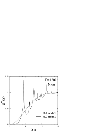
FIG. 3.: Inelastic part of the structure factor at $\Gamma=180$ for classical bcc crystal.

Thus, in a crystal, the inelastic part of the structure factor, $S^{\prime\prime}(k)$, appears to be singular in addition to the Bragg (elastic) part $S^{\prime}(k)$. The singularities of $S^{\prime\prime}(k)$ are weaker than the Bragg diffraction delta functions in $S^{\prime}(k)$; the positions of singularities of both types coincide. The pronounced shapes of the $S^{\prime\prime}(k)$ peaks may, in principle, enable one to observe them experimentally. The structure factor $S(k)$ in the Coulomb liquid (see, e.g., Ref. [17] and references therein) also contains significant but finite and regular humps associated with short-range order. This structure has been studied in detail by MC and other numerical methods. In contrast, the studies of singular structure factors in a crystal by MC or MD methods would be very complicated. Luckily, they can be explored by the HL model.

Finally, it is instructive to compare the behavior of $S^{\prime\prime}(k)$ at small $k$ in the HL1 and HL2 models. It is easy to see that the main contribution to inelastic scattering at these $k$ comes from one-phonon normal processes [with q=k in Eq. (64)]. At these $k$ the HL2 $S^{\prime\prime}_{2}(k)$ coincides with the one-phonon $S^{\prime\prime}_{\rm 1ph}(k)$ and with the static structure factor of Coulomb liquid (at the same $\Gamma$) and reproduces correct hydrodynamic limit [18], $S(k)\propto k^{2}$. The HL1 model, on the contrary, overestimates the importance of the normal processes.

Let us mention that we have also used the HL2 model to calculate $g(r)$. HL2 appears less accurate than HL but better than HL1. We do not plot $g_{2}(r)$ to avoid obscuring the figures.

VI Conclusions

Thus, the harmonic lattice model allows one to study static and dynamic properties of quantum and classical Coulomb crystals. The model is relatively simple, especially in comparison with numerical methods like MC, PIMC and MD. The model can be considered as complementary to the traditional numerical methods. Moreover, it can be used to explore dynamic properties of the Coulomb crystals and quantum effects in the cases where the use of numerical methods is especially complicated. For instance, the harmonic lattice model predicts singularities of the static inelastic structure factor at the positions of Bragg diffraction peaks. We expect also that the HL model can describe accurately non-Coulomb crystals whose lattice vibration properties are well determined.

Acknowledgements. We are grateful to N. Ashcroft for discussions. The work of DAB and DGY was supported in part by RFBR (grant 99–02–18099), INTAS (96–0542), and KBN (2 P03D 014 13). The work of HEDW and WLS was performed under the auspices of the US Dept. of Energy under contract number W-7405-ENG-48 for the Lawrence Livermore National Laboratory and W-7405-ENG-36 for the Los Alamos National Laboratory.

REFERENCES

• [1] E.P. Wigner, Phys. Rev. 46, 1002 (1934).
• [2] S.Ya. Rakhmanov, Zh. Eksper. Teor. Fiz. 75, 160 (1978).
• [3] W.M. Itano, J.J. Bollinger, J.N. Tan, B. Jelenković, X.-P. Huang, and D.J. Wineland, Science 279, 686 (1998); D.H.E. Dubin and T.M. O’Neil, Rev. Mod. Phys. 71, 87 (1999).
• [4] G. Chabrier, Astrophys. J. 414, 695 (1993); G. Chabrier, N.W. Ashcroft, and H.E. DeWitt, Nature 360, 48 (1992).
• [5] G.S. Stringfellow, H.E. DeWitt, and W.L. Slattery, Phys. Rev. A41, 1105 (1990); W.L. Slattery, G.D. Doolen, and H.E. DeWitt, Phys. Rev. A21, 2087 (1980).
• [6] R.T. Farouki and S. Hamaguchi, Phys. Rev. E47, 4330 (1993).
• [7] S. Ogata, Astrophys. J. 481, 883 (1997).
• [8] D.A. Baiko, A.D. Kaminker, A.Y. Potekhin, and D.G. Yakovlev, Phys. Rev. Lett. 81, 5556 (1998).
• [9] C. Kittel, Quantum Theory of Solids (Wiley, New York, 1963).
• [10] D.A. Baiko and D.G. Yakovlev, Astron. Lett. 21, 702 (1995).
• [11] R.C. Albers and J.E. Gubernatis, preprint of the LASL LA-8674-MS (1981).
• [12] M. Born and K. Huang, Dynamical theory of crystal lattices (Claredon Press, Oxford, 1954).
• [13] D.H.E. Dubin, Phys. Rev. A42, 4972 (1990).
• [14] H. Nagara, Y. Nagata, and T. Nakamura, Phys. Rev. A36, 1859 (1987).
• [15] R.C. Albers and J.E. Gubernatis, Phys. Rev. B23, 2782 (1981).
• [16] G. Chabrier and A.Y. Potekhin, Phys. Rev. E58, 4941 (1998).
• [17] D.A. Young, E.M. Corey, and H.E. DeWitt, Phys. Rev. A44, 6508 (1991)
• [18] P. Vieillefosse and J.P. Hansen, Phys. Rev. A12, 1106 (1975)