A Monte Carlo code for full simulation of a transition radiation detector

Abstract

A full simulation of a transition radiation detector (TRD) based on the GEANT, GARFIELD, MAGBOLTZ and HEED codes has been developed. This simulation can be used to study and develop TRD for high energy particle identification using either the cluster counting or the total charge measurement method. In this article it will be also shown an application of this simulation to the discrimination of electrons from hadrons in beams of momentum of few $GeV/c$ or less, assuming typical TRD configuration, namely radiator–detector modules.

(To be submitted to Computer Physics Communication)

1 Introduction

Transition radiation (TR) is an electromagnetic radiation produced by ultrarelativistic charged particles crossing the interface between two materials with different dielectric properties [1, 2]. The TR spectrum is peaked in the X-ray region and the probability of a X-ray photon being emitted at each interface is of the order of $\alpha\simeq 1/137$. The transition radiation yield is proportional to the Lorentz factor $\gamma$ of the incident charged particle and is independent on the kind of particle. That offers an attractive alternative to identify particles of given momentum with a non destructive method.

In order to enhance the TR X-ray production, radiators consisting of several hundred foils regularly spaced or irregular radiators of few $cm$ of thickness consisting of carbon compound foam layers or fiber mats are usually adopted. The “multilayer” radiator introduces significant physical constraints on the radiation yield, because of the so-called “interference effects”. It has been established that the radiation emission threshold occurs at a Lorentz factor $\gamma_{th}=2.5\omega_{p}d_{1}$, where $\omega_{p}$ is the plasma frequency (in $\,{\rm eV}$ units) of the foil material, and $d_{1}$ is its thickness in $\,{\rm\mu m}$. For $\gamma\geq\gamma_{th}$ the radiation yield increases up to a saturation value given by $\gamma_{sat}\sim\gamma_{th}(d_{2}/d_{1})^{1/2}$, where $d_{2}$ is the width of the gap between the foils [3].

The conventional method of TR detection is the measurement of the sum of the energy released by ionization and from photoelectrons produced by TR X-rays. The radiating particle, if not deflected by magnetic fields, releases its ionization energy in the same region as the X-ray photons, introducing a background signal that can be reduced if a gaseous detector is used. Since the gas must provide efficient conversion of the TR photons, the use of high-Z gases is preferred. The detector usually consists of proportional chambers filled with argon or xenon with a small addition of quenching gases for gain stabilization ($CO_{2}$, $CH_{4}$).

The measurement of TR using proportional chambers is generally based on one or both of the following methods:

• the “charge measurement” method, where the signal collected from a chamber wire is charge analyzed by ADCs [4];

• the “cluster counting” method, where the wire signal is sharply differentiated in order to discriminate the X-ray photoelectron clusters producing pulses (hits) exceeding a threshold amplitude from the $\delta$-ray ionization background [5].

In both cases a cut on the analyzed charge or on the number of clusters is needed in order to discriminate radiating particles from slower nonradiating ones. Multiple module TRDs, with optimized gas layer thickness, are normally employed to improve background rejection. A reduced chamber gap limits the particle ionizing energy losses, while the X-rays escaping detection may be converted in the downstream chambers.

Transition radiation detectors are presently of interest in fast particle identification, both in accelerator experiments [6, 7] and in cosmic ray physics [8]-[16]. A TRD is used to evaluate the underground cosmic ray muon energy spectrum in the Gran Sasso National Laboratory [17]. In spite of their use in several high energy experiments, a simulation code is not yet available in the standard simulation tools.

Several codes based on parameterizations of test beam measurements have been developed to simulate the TRDs [18, 19]. Lately a TRD has been proposed in a Long Base Neutrino Oscillation Experiment [20], in which a simulation has been developed using a GEANT interface [21]. The results achieved in the last experience have been rather satisfactory, in spite of some difficulties to track low energy photons in GEANT.

In this paper a full simulation of a TRD is described. The program is based on GEANT [22], GARFIELD [23], MAGBOLTZ [24] and HEED [25] codes in order to exploit the best performances in each one. In this way a full simulation has been developed tracking the particles into the detector and producing the pulse shape from each proportional tubes.

2 Transition radiation emission

Extensive theoretical studies have been made about TR. The basic properties of the TR production as well as the interference phenomena in multifoil radiator stacks are rather well understood and well described with classical electromagnetism (for instance see [26]). There was also an attempt to give a quantum description of TR [27]. The quantum corrections to the TR intensity become interesting for the emission of very high energy photons, namely when the TR photon energy is comparable with the energy of the radiating particle. Therefore they are no longer significant in the X-ray region for incident charged particle of momenta of few $GeV/c$ and the expressions derived are similar to the classical theory. Therefore, the TR emission is described for practical purposes by classical formulation, and the TR energy is considered carried out by photons (quanta).

As shown by Artru et al. [3] the TR energy $W$ emitted from a stack of $N$ foils of thickness $d_{1}$ at regular distances $d_{2}$, without taking into account absorption effects, can be written as:

$$\cfrac{d^{2}W}{d\omega~{}d\theta^{2}}=\eta~{}4~{}\sin^{2}{\cfrac{\phi_{1}}{2}}\left(\dfrac{\sin{N~{}\cfrac{\phi}{2}}}{\sin{\cfrac{\phi}{2}}}\right)^{2}$$ (1)

Where

$$\eta=\frac{\alpha}{\pi}\left(\frac{1}{\gamma^{-2}+\theta^{2}+\xi_{1}^{2}}-\frac{1}{\gamma^{-2}+\theta^{2}+\xi_{2}^{2}}\right)^{2}\theta^{2}$$ (2)

is the energy emitted at each interface. In eq. (1) and (2) $\theta$ is the angle between the incident particle and the TR X-ray, and $\xi_{i}=\omega_{i}/\omega$ where $\omega$ is the TR quantum energy (in $\,{\rm eV}$ units) and $\omega_{i}$ are the plasma energies of the two media “1” (foil) and “2” (gap).

The factor $4~{}\sin^{2}{\cfrac{\phi_{1}}{2}}$ in eq. (1) is due to the coherent superposition of TR fields generated at the two interfaces of one foil, with the phase angle $\phi_{1}=d_{1}/z_{1}$ being the ratio of the foil thickness $d_{1}$ (in $\,{\rm\mu m}$ units) to the “formation zone” $z_{1}$ of the foil material:

$$z_{1}=\left(2.5~{}\omega~{}(\gamma^{-2}+\theta^{2}+\xi_{1}^{2})\right)^{-1}$$ (3)

The last factor of eq. (1) describes the coherent interference of TR in a stack composed of $N$ foils and gaps at regular distances $d_{2}$. $\phi=\phi_{1}+\phi_{2}$ is the total phase angle of one basic foil plus gap, with $\phi_{2}$ being defined in analogy to $\phi_{1}$. The TR X-ray energy distribution can be obtained by taking the ratio of equation (1) to $\omega$.

Since the TR yield from multifoil stack is described as an interference phenomenon due to whole radiator, in order to calculate the total TR quanta emitted by the particle crossing the radiator, one needs to known the total number of foils crossed. Therefore it is not possible to follow the particle into radiator in order to calculate the probability to emit a quantum in a given step, i.e. we do not have a cross section for the TR effect. That may introduce some difficulties to simulate the TR process. Moreover, the TR intensity is a complex function of the thicknesses $d_{1}$ and $d_{2}$, of the plasma energies $\omega_{1}$ and $\omega_{2}$ for a given $\gamma$ Lorentz factor. This behaviour may introduce an additional difficulty to calculate the TR spectra for any kind of radiators.

The energy of the TR photons depends on the radiator material and its structure. In ref. [3] it is shown that the average TR energy carried out by quanta is given by:

$$<\omega>\simeq 0.3~{}\gamma_{th}~{}\omega_{1}$$ (4)

Assuming $d_{1}=10~{}\mu m$ and $\omega_{1}=20~{}eV$ one obtains $\gamma_{th}\sim 500$ and $<\omega>\sim 3~{}keV$. This may introduce some difficulties to track soft X-ray photons in a medium.

The ability to identify particles by a TRD is determined by the relative amounts of TR and ionization energy loss in the proportional chambers. Large fluctuations of ionization loss in thin gas layers limit this methods. Therefore, in order to better understand the performance of a TRD, one needs careful calculations of ionization energy loss and its fluctuations, producing knock-on or $\delta$-electrons. On the other hand, if one would like to use the cluster counting method to separate the TR X-ray from the track ionization background, then the range and the size of $\delta$-electron and of photoelectron, the number of electron–ion pairs produced in the gas and their arrival time on the wire need to be taken into account. Finally the current produced on the anode wire of the gas chambers and its pulse shape fed to discriminator by the front end electronics also play an important role in this method.

3 TRD full simulation

On the basis of the above discussion, the approach followed to simulate a TRD is based on the codes GEANT, GARFIELD, MAGBOLTZ and HEED (the last two codes are used by GARFIELD). The geometric description of the detector has been given by GEANT, including the simulation of all physical processes that occur in the materials crossed by the particles. The ionization energy loss and the photoelectric process in the gas have been not considerated in the GEANT code, because they are simulated by HEED.

When charged particles cross the gas of proportional chambers, or photons are entering into these volumes, the HEED package is called. In this way the ionization energy loss and the electron–ion pairs distribution along the track are calculated. The photoelectric absorption of photons in the gas is also simulated, including the evaluation of the photoelectrons produced and the total number of electron–ion pairs. Finally the current pulse produced on the anode wire is evaluated by the GARFIELD code using the gas properties as its drift velocity and gain calculated by the MAGBOLTZ program as a function of the electric field.

3.1 TR process

The GEANT code does not simulate transition radiation. In order to produce the TR photons in GEANT, a physical process has been introduced whenever a relativistic charged particle crosses the radiator.

The TR photon energy spectrum and the mean number of X-ray are calculated for the input radiator and for the energy of primary particle which one simulates. When the charged particle crosses the radiator and comes out the TR process is activated. The total number of TR photons is generated according to a Poisson distribution if their average number is less than 10, otherwise a Gaussian distribution may be used. The energy of each TR X-ray is randomly generated according to a calculated spectrum and its position is generated along the radiating particle path at the end of a radiator. The produced TR photons are then treated as secondary particles in GEANT and they are stored in the common block GCKING. In order to be transported by GEANT, these photons are stored in the data structure JSTAK by the GSKING routine.

3.1.1 TR formulas used in the code

The TR production relations used in this simulation take into account the photon absorption in the radiator. This effect has been simulated using the GEANT absorption lengths of the photons calculated for this material.

Regular radiator
The energy distribution of TR photons for a stack of plates taking into account the absorption in the foils and gaps is given by [3]:

$$\cfrac{d^{2}N}{d\omega~{}d\theta^{2}}=\cfrac{1}{\omega}~{}\eta~{}4~{}\sin^{2}{\cfrac{\phi_{1}}{2}}\left(\cfrac{\sin^{2}{N~{}\cfrac{\phi}{2}}+\sinh^{2}{N~{}\cfrac{\sigma}{2}}}{\sin^{2}{\cfrac{\phi}{2}}+\sinh^{2}{\cfrac{\sigma}{2}}}\right)\e^{-\frac{N-1}{2}~{}\sigma}$$ (5)

where $\sigma=d_{1}/\lambda_{1}+d_{2}/\lambda_{2}$ is the absorption in one foil + one gap and $\lambda_{1}$ and $\lambda_{2}$ are the absorption lengths for the emitted radiation in two media as calculated by GEANT (see paragraph 3.2).

For large values of the number of foils $N$, the $\delta$ function can be assumed to approximate the last two factors of the above expression. Making this approximation and integrating over $\theta^{2}$, equation (5) becomes:

$$\cfrac{dN}{d\omega}=\cfrac{1}{\omega}~{}\cfrac{4~{}\alpha~{}N_{equ}}{1+\tau}\sum_{n}\theta_{n}\left(\cfrac{1}{\rho_{1}+\theta_{n}}-\cfrac{1}{\rho_{2}+\theta_{n}}\right)^{2}\left(1-\cos{(\rho_{1}+\theta_{n})}\right)$$ (6)

where

$\rho_{i}=2.5~{}d_{1}~{}\omega~{}(\gamma^{-2}+\xi_{i}^{2})$;

$\tau=d_{2}/d_{1}$;

$\theta_{n}=\cfrac{2~{}\pi~{}n-(\rho_{1}+\tau\rho_{2})}{1+\tau}>0$;

$N_{equ}=\cfrac{1-\e^{-N\sigma}}{1-\e^{-\sigma}}$  .

$N_{equ}$ is the number of equivalent foils when the absorption is take into account.

To evaluate the total number of TR photons the numerical calculation of equation (6) has been carried out at selected X-ray energies ($\omega$), from $1~{}keV$ to $100~{}keV$, with a precision better than $10^{-3}$. In Fig. 1 the TR spectra for a regular radiator, evaluated taking into account the absorption in the radiator, are shown. They are calculated from the eq. (6). This figure shows a broad peak around $3-5~{}keV$ energy, corresponding to TR mean energy produced by the regular radiator adopted.

Irregular radiator
The transition radiation has been observed in irregular materials consisting for instance of plastic foams. A general formulation of the spectral distribution of the number of TR X-ray quanta produced in a irregular medium, consisting of randomly parralel plates of arbitrary thickness, is given by Garibian et al. [28]. This formulation has been given with the plates arranged in vacuum. It has been modified to take into account the presence of a material in the gap.

The average number of radiation quanta taking into account the absorption of the radiation is given by:

$$<\cfrac{d^{2}N}{d\omega~{}d\theta}>=\cfrac{2~{}\alpha}{\pi~{}\omega}\left(\cfrac{1}{1-\beta^{2}~{}\epsilon_{1}+\theta^{2}}-\cfrac{1}{1-\beta^{2}~{}\epsilon_{2}+\theta^{2}}\right)^{2}\theta^{3}I$$ (7)

Here

$$I=2~{}\cfrac{1-p^{N}}{1-p}~{}Re\cfrac{(\cfrac{1+p}{2}-h_{1})-(p-h_{1}~{}\cfrac{1+p}{2})~{}h_{2}}{1-h_{1}~{}h_{2}}+$$ (8)

$$2~{}Re\cfrac{(1-h_{1})~{}(p-h_{1})~{}h_{2}~{}(p^{N}-h_{1}^{N}~{}h_{2}^{N})}{(1-h_{1}~{}h_{2})~{}(p-h_{1}~{}h_{2})}$$

is the factor due to the superpositions of the radiation fields in the plates and in the gap. The other parameters are:

$\epsilon_{k}=1-(\omega_{k}/\omega)^{2}+i/(5~{}\lambda_{k}~{}\omega)$;

$h_{k}=<\e^{-i~{}\phi_{k}~{}d_{k}}>$;

$\phi_{k}=5~{}\omega~{}\left(\beta^{-1}-\sqrt{\epsilon_{k}-\sin^{2}{\theta}}\right)=\phi^{\prime}_{k}+i\phi^{\prime\prime}_{k}$;

$p=<\e^{-d_{1}/\lambda_{1}}>~{}<\e^{-d_{2}/\lambda_{2}}>$.

The angle brackets denote the averaging of random quantities with a distribution determined by the distributions of $d_{1}$ and $d_{2}$.

For most of foam radiators the random foil and the gap thickness can be described by a gamma distribution [29]. In this way one finds that [28]:

$h_{k}=|h_{k}|~{}\e^{i~{}\psi_{k}}$;

$|h_{k}|=\left(\left(1+\cfrac{<d_{k}>}{2~{}\lambda_{k}~{}\alpha_{k}}\right)^{2}+\left(\cfrac{\phi^{\prime}_{k}~{}<d_{k}>}{\alpha_{k}}\right)^{2}\right)^{-\alpha_{k}/2}$;

$\psi_{k}=-\alpha_{k}~{}arctg~{}\cfrac{\phi^{\prime}_{k}~{}<d_{k}>}{\alpha_{k}+<d_{k}>/(2~{}\lambda_{k})}$;

$p=\left(1+\cfrac{<d_{1}>}{\lambda_{1}~{}\alpha_{1}}\right)^{-\alpha_{1}}~{}\left(1+\cfrac{<d_{2}>}{\lambda_{2}~{}\alpha_{2}}\right)^{-\alpha_{2}}$.

The parameters $\alpha_{k}$ represent the degree of irregularity: $\alpha_{k}=(<d_{k}>/\sigma_{k})^{2}$ where $<d_{k}>$ and $\sigma_{k}$ are the mean values and the mean squared deviations respectively of foil ($k=1$) and gap ($k=2$) thickness distributions.

3.2 Use of the GEANT package

The GEANT 3.21 code is used to describe the geometrical volumes inside the detector and to define the materials. It has been done by the standard GEANT routine taking care of tracking parameters in order to define the active physical processes and the cuts (GSTPAR). In this way, the photons are tracked using the GEANT absorption coefficients and the gamma cuts have been lowered to $1~{}keV$ in all the materials.

The materials used, which are not defined in the default GEANT program, have been implemented using the standard routine (GSMATE or GSMIXT). The radiators have been defined as a mixture composed by the foil material and the gap material (air) containing the proportion by weights of each material. The foil materials and the gas chamber walls have been defined as compounds containing the proportion by number of atoms of each kind [22].

In Fig. 2 the photon attenuation lengths calculated by GEANT for polyethylene ($CH_{2}$, $\rho=0.93~{}g/cm^{3}$), kapton ($C_{22}H_{10}N_{2}O_{5}$, $\rho=1.42~{}g/cm^{3}$) and mylar ($C_{5}H_{4}O_{2}$, $\rho=1.05~{}g/cm^{3}$) are shown. In this figure one can see that the kapton photon attenuation length is always less than polyethylene and the photon attenuation length for kapton is the same as for mylar.

The gas chambers are the sensitive volume of the TRD and for each charged particle crossing the gas or for each photons absorbed inside, a GEANT HITS structure is defined to describe the interaction between particle and detector. In the HITS structure the following information are stored:

• HITS(1) = number of volume level (by GEANT);

• HITS(2) = energy loss in the gas (by HEED);

• HITS(3) = input time in the volumes (by GEANT);

• HITS(4:6) = x, y and z of entry point in the volume (by GEANT);

• HITS(7:9) = x, y and z of exit point in the volume (by GEANT);

• HITS(10) = number of cluster produced in the gas (by HEED);

• HITS(11) = number of electron–ion pairs produced in the gas (by HEED);

• HITS(12:111) = current pulse on the wire for 100 time slices (by GARFIELD).

The DIGIT structure is similar to the HITS one, where the information are stored as a sum of all particles crossing that volume, while the input and the output coordinate are relative to the primary particle which has crossed the chamber.

The event processing is a highly CPU consuming job. To optimize CPU usage DST files are produced to be analyzed at a later time. For each event the GEANT ZEBRA data structures containing the geometrical definition, the input kinematics, the tracking banks (JXYZ) and the simulated detector response (HITS and DIGIT banks) are stored in DST files which provide the input data set for the analyses to be performed. In this way, the electronic response of the chamber front end can be implemented starting by the anode current impulse. In order to save some run informations the HEADER bank is also used by the GSRUNG routine.

3.3 Use of the GARFIELD package

The GARFIELD program has been developed to simulate gaseous wire chambers operating in proportional mode. It can be used for instance to calculate the field maps and the signals induced by charged particles, taking both electron pulse and ion tail into account. An interface to the MAGBOLTZ program is provided for the computation of electron transport properties in nearly arbitrary gas mixtures. Starting from version 6, GARFIELD has also an interface with the HEED program to simulate ionization of gas molecules by particles traversing the gas chamber. A few examples of GARFIELD results can find via WWW [23, 25].

The HEED program computes in detail the energy loss of fast charged particles in gases, taking $\delta$-electrons and optionally multiple scattering of the incoming particle into account. The program can also simulate the absorption of photons through photo-ionization in gaseous detectors. From this program, the distribution of electron–ion pairs along the particle track length in the gas has been computed by GARFIELD. Some modifications have been included in the GARFIELD default version in order to calculate the cluster size distribution of photons absorbed in the gas by HEED. Starting from these cluster size distributions the current anode wire signal is calculated by GARFIELD.

In Fig. 3 the pair distribution produced by $5.9~{}keV$ photons ($\@@nuc{55}{Fe}$) in $1~{}cm$ of xenon at NTP is shown. From this figure one can see the presence of a mean peak of about 270 electron–ion pairs due to the photoelectron and the Auger electron. There is also a secondary peak due to occasional detection of a photoelectron whitout Auger emission.

In this TRD simulation the GARFIELD 6.27 version has been used. From the source files of GARFIELD program, written in Fortran 77 and Patchy as pre-processor, the main routines have been included in the code together with the GEANT routines. Some modifications have been introduced in order to skip interactive input information used by GARFIELD. All information to run the program are given via FFREAD data card. The cell definition and the gas composition of the chambers to be simulated have been processed in initialization of the program.

4 Program description

The main items of this simulation have already been described in the above discussion. In this section an example of how the program works is given. It has been written in Fortran by patchy as pre-processor on a PC $166~{}MHz$, $80~{}MB$ of RAM, in the LINUX system (RedHat 5.2 version). It is transportable on any system changing some patchy control flags in cradle files.

There are two codes: the first is dedicated to event simulation for DST production; the second one is used to analyze the DST files including a graphical interface too. The input of these program is given via data cards by FFREAD facility. The user inputs for the first program are stored in the run header bank after the initialization to be used by the second one.

4.1 Geometry

The geometry used to simulate a TRD consists of 10 radiator-proportional chamber modules. The radiator consists of 250 polyethylene foils of $5~{}\mu m$ of thickness at regular distances of $200~{}\mu m$ in air. The chamber consists of two planes of 16 cylindrical proportional tubes each of $2~{}mm$ of radius (straw tubes) to form a double layer close pack configuration. These tubes are widely used in recent high energy physics experiments [19, 30]. Since the typical materials used for the tube wall are made by carbon compounds (kapton, mylar and polycarbonate) and their thickness are typically $30-50~{}\mu m$, the straw tubes are good candidate to be used as X-ray detector due to the reduced attenuation length of the wall.

In this simulation the straw tube walls are made of kapton of $30~{}\mu m$ thickness internally coated with copper of $0.3~{}\mu m$ thickness. The anode wire used is of $25~{}\mu m$ thickness. The gas mixture used is based on $Xe(80\%)-CO_{2}(20\%)$ at atmospheric pressure. The anode voltage used is $1450~{}Volt$ which corresponds to a gas gain of about $2\cdot 10^{4}$.

4.2 Front end electronic

The front end electronic used in this simulation consists of a simply amplifier which is described by a low band-pass transfer function with a bandwidth of $50~{}MHz$ and an overall gain of 10:

$$\tilde{A}(\omega)=A_{0}\cfrac{1}{1+i\cfrac{\omega}{\omega_{0}}}$$ (9)

where $A_{0}=10~{}mV/\mu A$ and $\omega_{0}=50~{}MHz$.

The anode current produced in the proportional tubes as a function of the time $I(t)$ is converted in the output voltage amplitude $V(t)$ by:

$$V(t)=\int_{t}^{\infty}I(t^{\prime})~{}A(t-t^{\prime})~{}dt^{\prime}$$ (10)

where $A(t)$ is the Fourier transform of $\tilde{A}(\omega)$:

$$A(t)=\left\{\begin{array}[]{ll}\omega_{0}~{}\e^{-\omega_{0}~{}t}&,~{}if~{}t\geq 0\\ 0&,~{}otherwise\end{array}\right.$$ (11)

In this example no noise is assumed. Of course a real electronics is described by a more complex transfer function with an electronic noise.

In Fig. 4 a typical anode signal from a tube produced by a X-ray of $5.9~{}keV$ ($\@@nuc{55}{Fe}$) is shown. When this signal is processed by the low band-pass it assumes the shape reported in Fig. 5. From this figure one can see that the electronics performed a formation of the input signal with a FWHM of about $25~{}nsec$.

In Fig. 6 is shown a typically anode signal produced by a charged particle crossing a tube. In this figure one can see two peaks are produced by two clusters. The low band-pass cannot allow to distinguish the two clusters since the second one is superimposed to first one (signal pile-up) as shown in Fig. 7, because their time distance is lower than the FWHM of the electronic resolution.

4.3 Results

In this paragraph the results achieved by the TRD geometry defined above are shown. In Fig. 8 the average energy loss (summed over 10 planes) as function of the Lorentz factor is shown. This result has been obtained by simulating pions and electrons of different energies with or without radiators. For each energy 1000 events have been simulated.

In this figure one can see that the yield increases with $\gamma$ when the radiators are arranged before the proportional tubes. The TR saturation is achieved at $\gamma\simeq 8000$. For $\gamma$ less than 100–500 only the ionization is released in the gas, as is shown in the same figure.

In Fig. 9 the average energy loss distributions (summed over 10 planes) for electrons of $4~{}GeV/c$ and pions of $255~{}MeV/c$ are shown. From this figure it is possible to see that the average value of the electron distribution is greater than the average for pions. This is due to presence of the X-ray TR produced in the radiator by the electrons.

In order to perform the cluster size analysis, one needs to know the relationship between the output signal amplitude and the energy loss in the tube. Therefore an analysis of voltage amplitude has been done using X-rays of $5.9~{}keV$ ($\@@nuc{55}{Fe}$). In Fig. 10 is shown the output voltage amplitude distribution produced by a $\@@nuc{55}{Fe}$ X-rays absorbed in a proportional tube. From this figure one can see that the energy loss of $5.9~{}keV$ corresponds to $170~{}mV$ of output voltage amplitude.

In order to count the number of hits produced for instance by TR photons and by $\delta$-ray with energy greater than $5~{}keV$, a cut of $145~{}mV$ is imposed to the voltage amplitude signal produced in each tube. In Fig. 11 the average total number of hits (summed over all fired tubes) when the output signal is greater than $145~{}mV$ as function of $\gamma$ is shown. The behaviour of the TRD when is analyzed by the cluster counting method is similar to the charge measurement one.

In Fig. 12 the distributions of the total number of hits for electrons of $4~{}GeV/c$ and pions of $255~{}MeV/c$ are shown. Again we can observe that the average value of the electron distribution is greater than the one of the pion distribution, due to presence of the X-ray TR produced in the radiator by the electrons.

In order to discriminate electrons from pions at given momentum by charge measurement or by cluster counting, we can use this simulation to optimize the gas thickness, the radiator, the threshold and the number of modules. In this way, we can optimize one of these methods or we can use more sophisticated ones, for example analyzing the pulse shape as function of the drift time or using the likelihood and/or neural network analysis by the pattern information, namely the fired tube configuration in the TRD.

5 Conclusions

A full simulation of a transition radiation detector (TRD) based on the GEANT, GARFIELD, MAGBOLTZ and HEED codes has been developed. The simulation can be used to study and develop TRD for high energy particle identification using either the cluster counting or the total charge measurement method. The program works very well according to the design expectations. It is quite flexible and it can be used to simulate any detector which is based on proportional counters, providing a very useful simulation tool.

Figure 1: The TR spectra generated by 250 foils of polyethylene ($d_{1}=5~{}\mu m$ and $\omega_{1}=20~{}eV$) at regular distances $d_{2}=200~{}\mu m$ in air ($\omega_{2}=0.7~{}eV$). Solid line: $\gamma=5000$; dashed line: $\gamma=1000$ and dotted line: $\gamma=500$.

Figure 2: Photon attenuation length for different materials as calculated by GEANT routines in the range from $1~{}keV$ to $100~{}keV$. Solid line: polyethylene; dashed line: kapton and dotted line: mylar.

Figure 3: Electron–ion pairs distribution for $1~{}cm$ of xenon at NTP produced by photons of $5.9~{}keV$ ($\@@nuc{55}{Fe}$).

Figure 4: Anode current signal produced by a X-ray of $5.9~{}keV$ absorbed in a tube.

Figure 5: Output amplitude voltage produced by a X-ray of $5.9~{}keV$ absorbed in a tube as processed by the low band-pass electronic.

Figure 6: Anode current signal produced by a charged particle crossing a tube.

Figure 7: Output amplitude voltage produced by a charged particle crossing a tube as processed by the low band-pass electronic.

Figure 8: Average energy loss (summed over 10 planes) as a function of the Lorentz factor. The error bars have been evaluated as ratio of the RMS over the square root of the number of events.

Figure 9: Average energy loss (summed over 10 planes) distribution for two $\gamma$ values. Solid line: pions of $255~{}MeV/c$; dashed line: electrons of $4~{}GeV/c$

Figure 10: Output voltage amplitude distribution (histogram) produced by X-rays of $5.9~{}keV$. The line is the result of a Gaussian fit

Figure 11: Total number of hits with a signal greater than $145~{}mV$ as a function of the Lorentz factor. The error bars have been evaluated as ratio of the RMS over the square root of the number of events.

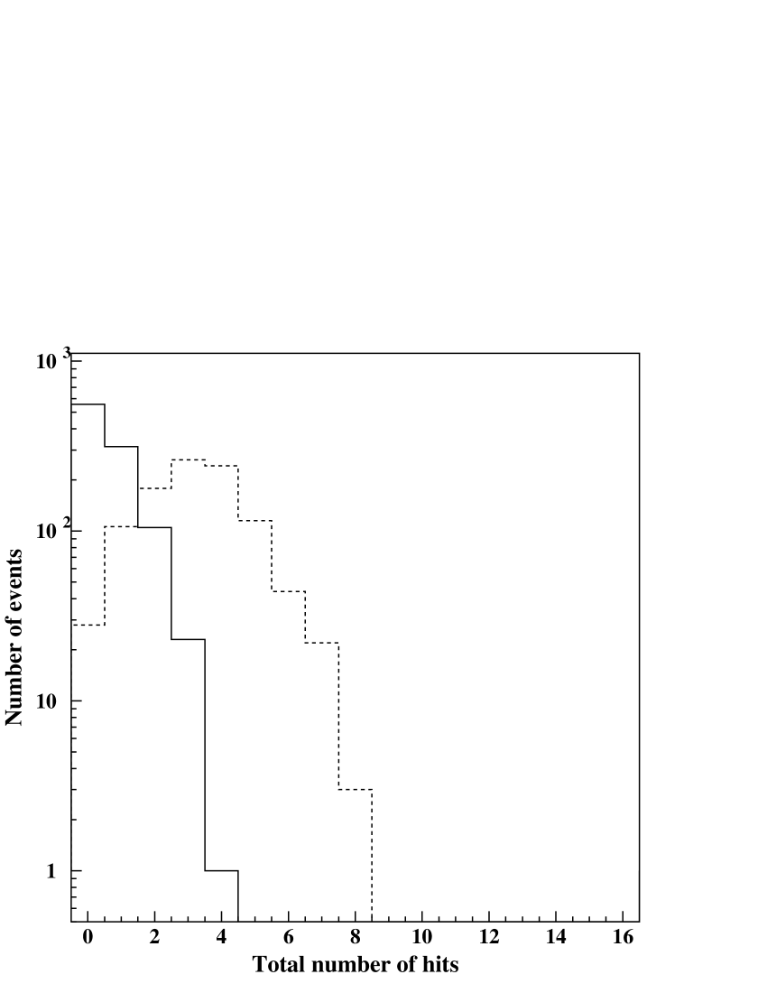
Figure 12: Hits distribution for two $\gamma$ values. Solid line: pions of $255~{}MeV/c$; dashed line: electrons of $4~{}GeV/c$

References

- [1] V. L. Ginzburg and I. M. Frank, JETP 16 (1946) 15
- [2] G. M. Garibian, Sov. Phys. JETP 6 (1958) 1079
- [3] X. Artru et al., Phys. Rev. D 12 (1975) 1289
- [4] J. Fischer et al., Nucl. Instr. and Meth. 127 (1975) 525
- [5] T. Ludlam et al., Nucl. Instr. and Meth. 181 (1981) 413
- [6] C. Camps et al., Nucl. Instr. and Meth. 131 (1975) 411
- [7] B. Dolgoshein, Nucl. Instr. and Meth. A 326 (1993) 434
- [8] T. A. Prince et al., Nucl. Instr. and Meth. 123 (1975) 231
- [9] G. Hartman et al., Phys. Rev. Lett. 38 (1977) 368
- [10] S. P. Swordy et al., Nucl. Instr. and Meth. 193 (1982) 591
- [11] K. K. Tang, The Astroph. Journ. 278 (1984) 881
- [12] J. L’Heureux, Nucl. Instr. and Meth. A 295 (1990) 245
- [13] S. W. Barwick et al., Nucl. Instr. and Meth. A 400 (1997) 34
- [14] R. L. Golden et al., The Astr. Journ. 457 (1996) L103
- [15] E. Barbarito et al. Nucl. Instr. and Meth. A 313 (1992) 295
- [16] E. Barbarito et al. Nucl. Instr. and Meth. A 357 (1995) 588
- [17] E. Barbarito et al. Nucl. Instr. and Meth. A 365 (1995) 214; The MACRO Collaboration (M. Ambrosio et al.), Proc. XXIV ICRC, Rome, 1 (1995) 1031; The MACRO Collaboration (M. Ambrosio et al.), Proc. XXV ICRC, Durban, (1997); The MACRO Collaboration (M. Ambrosio et al.), Nuclear Physics 61B (1998) 289; The MACRO Collaboration (M. Ambrosio et al.), Astroparticle Physics 10 (1999) 10; The MACRO Collaboration (M. Ambrosio et al.), Proc. XXVI ICRC, Salt Lake City, (1999), hep-ex 9905018
- [18] M. Castellano et al., Comput. Phys. Commun. 61 (1990) 395
- [19] T. Akesson et al., Nucl. Instr. and Meth. A 361 (1995) 440
- [20] G. Barbarino et al., The NOE detector for a long baseline neutrino oscillation experiment, INFN/AE-98/09 (1998)
- [21] P. Bernardini et al, GNOE: GEANT NOE simulation, Internal note 2/98 (1998) (unpublished)
- [22] R. Brun et al., CERN Publication DD/EE/84-1 (1992)
- [23] R. Veenhof, GARFIELD, a drift-chamber simulation program, W5050 (1999); http://consult.cern.ch/writeup/garfield/
- [24] S. Biagi MAGBOLTZ, a program to compute gas transport parameters W5050 (1997)
- [25] I. Smirnov, HEED, an ionization loss simulation program W5060 (1995); http://consult.cern.ch/writeup/heed/
- [26] C.W. Fabjan and W. Struczinski, Phys. Rev. Lett. 57B (1975) 483
- [27] G.M. Garibian, Sov. Phys. JETP 12 (1961) 1138
- [28] G.M. Garibian et al., Sov. Phys. JETP 39 (1974) 265
- [29] C.W. Fabjan, Nucl. Instr. and Meth. 146 (1977) 343
- [30] E. Barbarito et al. Nucl. Instr. and Meth. A 361 (1996) 39