Effective Field Theory for Highly Ionized Plasmas

Abstract

We examine the equilibrium properties of hot, non-relativistic plasmas. The partition function and density correlation functions of a plasma with several species are expressed in terms of a functional integral over electrostatic potential distributions. This is a convenient formulation for performing a perturbative expansion. The theory is made well-defined at every stage by employing dimensional regularization which, among other virtues, automatically removes the unphysical (infinite) Coulomb self-energy contributions. The leading order, field-theoretic tree approximation automatically includes the effects of Debye screening. No further partial resummations are needed for this effect. Subleading, one-loop corrections are easily evaluated. The two-loop corrections, however, have ultraviolet divergences. These correspond to the short-distance, logarithmic divergence which is encountered in the spatial integral of the Boltzmann exponential when it is expanded to third order in the Coulomb potential. Such divergences do not appear in the underlying quantum theory — they are rendered finite by quantum fluctuations. We show how such divergences may be removed and the correct finite theory obtained by introducing additional local interactions in the manner of modern effective quantum field theories. We compute the two-loop induced coupling by exploiting a non-compact $su(1,1)$ symmetry of the hydrogen atom. This enables us to obtain explicit results for density-density correlation functions through two-loop order and thermodynamic quantities through three-loop order. The induced couplings are shown to obey renormalization group equations, and these equations are used to characterize all leading logarithmic contributions in the theory. A linear combination of pressure plus energy and number densities is shown to be described by a field-theoretic anomaly. The effective Lagrangian method that we employ yields a simple demonstration that, at long distance, correlation functions have an algebraic fall off (because of quantum effects) rather than the exponential damping of classical Debye screening. We use the effective theory to compute, easily and explicitly, this leading long-distance behavior of density correlation functions.

The presentation is pedagogical and self-contained. The results for thermodynamic quantities at three-loop [or $O(n^{5/2})$] order, and for the leading long-distance forms of correlation functions, agree with previous results in the literature, but they are obtained in a novel and simple fashion using the effective field theory. In addition to the new construction of the effective field theory for plasma physics, we believe that the results we report for the explicit form of correlation functions at two-loop order, as well as the determination of higher-order leading-logarithmic contributions, are also original.

1 Introduction and Summary

Our work applies contemporary methods of effective quantum field theory to the traditional problem of a multicomponent, fully ionized hot (but non-relativistic) plasma. In this regime, a classical description might appear to suffice. But the short-distance ($1/r$) singularity of the Coulomb potential gives rise to divergences in higher-order terms. Taming these divergences requires the introduction of quantum mechanics. Quantum fluctuations smooth out the short-distance singularity of the Coulomb potential so that the quantum, many particle Coulomb system is completely finite. This necessity for including quantum effects, even in a dilute plasma, is discussed later in this introduction when the relevant parameters which characterize the various physical processes in the plasma are examined.

As we shall see, contemporary effective quantum field theory methods simplify high-order perturbative computations and generally illuminate the structure of the theory. Effective quantum field theories do, however, utilize a somewhat complicated formal apparatus involving regularization, counter terms, and renormalization. In an effort to make our work available to a wider audience, we shall develop the theory in several stages, and attempt to give a largely self-contained presentation. A brief review of some of the basic quantum field theory techniques used in our paper is presented in Appendix F. We begin, in Section 2, by casting the purely classical theory in terms of a functional integral. We show how dimensional continuation is convenient even at this purely classical level because it automatically and without any effort removes the infinite Coulomb self-energy contributions of the particles. The simple saddle-point evaluation of the functional integral — known as a tree approximation in quantum field theory — immediately gives Debye screening of the long-distance Coulomb potential without any need for the resummations appearing in traditional approaches. The first sub-leading, so-called “one-loop,” corrections to the plasma thermodynamics and correlation functions are also evaluated in this section. These lowest-order results are also used to illustrate general relations among correlations functions which are described more formally, and systematically, in Appendix A.

The divergence associated with the singular, short-range behavior of the Coulomb potential first arises at the subsequent, “two-loop” level of approximation as shown in Section 3. This section explains how the previous purely classical theory is obtained from a limit of the quantum theory, and how the quantum corrections that tame the classical divergences appear in the form of induced couplings that contain compensating divergences. This discussion uses various results on functional determinants and Green’s functions contained in Appendix B. Although it is relatively easy to construct the “counter terms” that render the classical theory finite, it is considerably more difficult to obtain the finite pieces in the induced couplings that ensure that a calculation in the effective theory correctly reproduces the corresponding result in the full quantum theory. In the latter part of this section the “matching conditions” for the leading two-loop induced couplings are derived, and the two-loop induced couplings are explicitly evaluated. The key to this evaluation is the exploitation of an $su(1,1)$ symmetry of the Coulomb problem, which permits one to derive a simple and explicit representation for the two-particle contribution to the density-density correlation function. This $su(1,1)$ symmetry, and its consequences, are presented in Appendix D. Section III concludes with an examination of the necessary inclusion in the effective theory of interactions involving non-zero frequency components of the electrostatic potential.

It is worth noting that our determination of the induced couplings is based on examining Fourier transforms of number-density correlation functions at small but non-vanishing wave number. We use this method because these functions — at non-vanishing wave number — may be computed in a strictly perturbative fashion without taking into account the Debye screening that is necessary to make the zero wave number limit of these correlation functions finite. Matching in this fashion enables us to use the simple pure Coulomb potential for which the exact group-theoretical techniques apply. Our procedure is roughly equivalent to computing the second-order virial coefficient for a pure Coulomb potential, except that this coefficient has a long-distance, infrared divergence. This logarithmic divergence is removed by Debye screening, but there is always the difficulty of determining the constant under the logarithm. Our method avoids this difficulty. Years ago, W. Ebeling [and later Ebeling working together with collaborators] computed the second-order virial coefficient for a pure Coulomb potential with a long-distance cutoff, and then related this quantity to other ladder approximation calculations so as to obtain results that are, except for one term, equivalent to, and consistent with, our results for the induced couplings. Their work is summarized in Ref. [4]. This seminal work is certainly very impressive and significant, but it is much more complex than our approach, and (at least in our view) is far more difficult to understand in detail.

With the leading induced couplings in hand, we turn in Section 4 to compute all the thermodynamic quantities and the density-density correlators to two-loop order. As far as we have been able to determine, the two-loop results for the density-density correlation functions obtained in Section 4 are new. Various integrals required for these computations are evaluated in Appendix C, and an alternative derivation of the two-loop thermodynamic results using compact functional methods appears in Appendix G.

The thermodynamic results are extended to the next, three-loop, order in Section 5. We give complete, explicit results for the pressure (or equation of state), Helmholtz free energy, and internal energy, as well as the relations between particle densities and chemical potentials in a general multi-component plasma. We also display the specializations of the equation of state for the cases of a binary electron-proton plasma, and a one component plasma (in the presence of a constant neutralizing background charge density). As discussed at the end of this section, a genuine classical limit exists only for the special case of a one-component plasma. As a check on our results, Appendix E presents an independent, self-contained calculation of the leading $O(\hbar^{2})$ corrections to the equation of state of a one-component plasma in the semi-classical regime.

Prior results in the literature, corresponding to our three-loop [or $O(n^{5/2})$] level of accuracy, for the free energy and/or the equation of state go back more than 25 years. The book by Kraeft, Kremp, Ebeling, and Röpke [6] quotes a result for the Helmholtz free energy which is nearly correct but omits one term. A fairly recent publication by Alastuey and Perez [7] contains the complete, correct expression for the Helmholtz free energy, to three loop order, with which we agree. Recent papers by DeWitt, Riemann, Schlanges, Sakakura, and Kraeft [8, 9, 10] report results for some, but not all, of the terms contained in the three-loop pressure. These partial results are consistent with our three-loop pressure, once an unpublished erratum of J. Riemann is taken into account.

Just as in any effective field theory, the induced couplings that must be introduced to remove the infinities of the classical plasma theory obey renormalization group equations. In Section 6 we show how these renormalization group equations may be employed to compute leading logarithmic terms in the partition function — terms involving powers of logarithms whose argument is the (assumed large) ratio of the Debye screening length to the quantum thermal wave length of the plasma. We show that, in general, log^k terms first arise at $2k$-loop order. We derive a simple recursion relation which determines their explicit form. We explicitly evaluate the coefficients of the logarithm-squared terms which arise at four and five loop order, and the log-cubed terms which appear at six loop order. The existence of these higher powers of logarithms which first appear at four loop order (where they correspond to $n^{3}\ln^{2}n$ contributions to the pressure) has often not been recognized. Recently, Ortner [12] has examined a classical plasma consisting of several species of positive ions moving in a fixed neutralizing background of negative charge. He computed the free energy to four-loop (or $n^{3}$) order and correctly obtained the $n^{3}\ln^{2}n$ term.

Since Planck’s constant, which carries the dimensions of action, does not appear in classical physics, fewer dimensionless ratios can be formed in a classical theory than in its quantum counterpart. In particular, the partition function of the classical theory depends upon a restricted number of dimensionless parameters, from which a linear relation between the pressure, internal energy, and average number densities follows. This relation is altered by the necessary quantum-mechanical corrections. Section 6 also explains how this alteration of the linear relationship is connected to “anomalies” brought about by the renormalization procedure that makes the classical theory finite.

We conclude our work, in Section 7, with an examination of the long-distance behavior of the density-density correlation function. Despite the presence of Debye screening, it is known that quantum fluctuations cause correlations to fall only algebraically with distance [14, 15, 16, 17]. Using the effective theory, we compute the coefficient of the resulting leading power-law decline in particle- and charge-density correlators in a very simple and efficient fashion, and obtain results which agree with previously reported asymptotic forms [16, 17].

It should be emphasized that the major purpose of this paper is to introduce the methods of modern effective field theory into the traditional field of plasma physics. Although many of the results that we derive and describe have been obtained previously, the methods that we employ to obtain these results are new, and they substantially reduce the computational effort as well as illuminating the general structure of the theory. Although our work may have the length, it is not a review paper; its length results from our desire to make the presentation self-contained so that it may be read by someone who is neither an expert in plasma physics nor quantum field theory. Since our work is not a survey of the field, we have not endeavored to provide anything resembling a comprehensive bibliography. For a recent review of known results concerning Coulomb plasmas at low density, including rigorous theorems and detailed discussion of the long distance form of correlators, we refer the reader to Ref. [18] and references therein.

1.1 Relevant Scales and Dimensionless Parameters

Various dimensionless parameters characterize the relative importance of different physical effects in the plasma. Before plunging into the details of our work, we first pause to introduce these parameters and discuss their significance.

Let $e$ and $n$ denote the charge and number density of a typical ionic species in the plasma. For simplicity of presentation in this qualitative discussion, we shall assume that the charges and densities of all species in the multicomponent plasma are roughly comparable, and shall ignore the sums over different species which should really be present in formulas such as (1.2) below. The subsequent quantitative treatment will, of course, remedy this sloppiness. We shall be concerned with neutral plasmas which are sufficiently dilute so that the average Coulomb energy of a particle is small compared to its kinetic energy. We use energy units to measure the temperature $T$ and write $\beta=1/T$. In the ideal gas limit, the average kinetic energy is equal to ${\textstyle{3\over 2}}T$. The Coulomb potential is $e^{2}/(4\pi r)$ in the rationalized units which we shall use. So the typical Coulomb energy is $e^{2}/(4\pi d)$ where $d\equiv n^{-1/3}$ denotes the mean inter-particle separation. Hence, the dimensionless parameter

$$\Gamma\equiv{e^{2}\over 4\pi d\,T}={\beta e^{2}\over 4\pi}\,n^{1/3}$$ (1.1)

is essentially the ratio of the potential to kinetic energy in the plasma, and it is an often used measure of the relative strength of Coulomb interactions in a plasma. However, we shall see that $\Gamma$ is not the proper dimensionless parameter which governs the size of corrections in the classical perturbation expansion.

A charge placed in the plasma is screened by induced charges. The screening length equals the inverse of the Debye wave number which we denote as $\kappa$. It is given (to lowest order in a dilute plasma) by

$$\kappa^{2}=\beta e^{2}n\,.$$ (1.2)

A different measure of the strength of Coulomb interactions in the plasma is defined by

$$g={\beta e^{2}\kappa\over 4\pi}\,.$$ (1.3)

This is the ratio of the electrostatic energy of two particles separated by a Debye screening length to the temperature (which is roughly the same as the average kinetic energy in the plasma). Equivalently, it is ratio of the “Coulomb distance”

$$d_{C}\equiv{\beta e^{2}\over 4\pi}$$ (1.4)

to the screening length $\kappa^{-1}$. The Coulomb distance $d_{C}$ is the separation at which the electrostatic potential energy of a pair of charges equals the temperature.

The number of particles $N_{\kappa}$ contained within a sphere whose radius equals the screening length $\kappa^{-1}$ is inversely related to $g$,

$$N_{\kappa}={4\pi\over 3}\,\kappa^{-3}\,n={1\over 3g}\,.$$ (1.5)

Hence the weak coupling condition $g\ll 1$ is equivalent to the requirement that the number of charges within a “screening volume” be large, $N_{\kappa}\gg 1$. In this case, a mean-field treatment of Debye screening holds to leading order, and perturbation theory is a controlled approximation.

It is easy to check that the two measures of interaction strength, $g$ and $\Gamma$, are related by $g=\sqrt{4\pi\,\Gamma^{\,3}}$. However, we shall show in our subsequent development that $g$, not $\Gamma$, is the dimensionless parameter whose increasing integer powers characterize the size of successive terms in the classical perturbative expansion for thermodynamic properties of the plasma. As we shall discuss, the classical perturbation series has a convenient graphical representation in which contributions at $n$-th order in perturbation theory are represented by graphs (or Feynman diagrams) with $n$ loops. We shall see that $g$ is the “loop expansion” parameter, such that contributions represented by $n$-loop graphs are of order $g^{n}$. Although $g$ and $\Gamma$ are directly related as noted above, we emphasize again that it is $g$ which is the correct classical expansion parameter.

To bring out this point even more strongly, we note that the screened Debye potential between two charges $e_{a}$ and $e_{b}$ a distance $r$ apart is given by $e_{a}e_{b}\,e^{-\kappa r}/(4\pi r)$. The modification of the self energy of a particle of charge $e_{a}$ when it is brought into the plasma is given by half the difference between the Debye potential and its Coulomb limit for the case of zero charge separation, ${\textstyle{1\over 2}}\lim_{r\to 0}\,(e_{a}^{2}/4\pi r)[e^{-\kappa r}-1]$, which is $-e_{a}^{2}\,\kappa/(8\pi)$. Each particle in the plasma makes this correction to the thermodynamic internal energy of the plasma, and so including this leading order correction to the energy density gives

$$u = {\sum}_{a}\left\{{3\over 2}\,T\,n_{a}-{e_{a}^{2}\kappa\over 8\pi}\,n_{a}\right\}$$ (1.6)

$$= T\,{\sum}_{a}\,n_{a}\left\{{3\over 2}-{\beta e_{a}^{2}\kappa\over 8\pi}\right\}\,,$$

which shows the appearance of $g$, or more explicitly $\beta e_{a}^{2}\kappa/(8\pi)$, as the correct Coulomb coupling constant in this case. This result for the internal energy which we have heuristically obtained agrees with the correct one-loop result (2.86) that is derived below.

A classical treatment of a plasma with purely Coulombic interactions is, however, never strictly valid. The classical partition function fails to exist due to the singular short-distance behavior of the Coulomb interaction. This can be seen in an elementary fashion directly from the divergence, for opposite signed charges, of the Boltzmann-weighted integral over the relative separation of two charges, $\int(d^{3}{\bf r})\>\exp\{\beta e^{2}/4\pi r\}$. In the perturbative expansion of the classical theory, this problem first manifests itself at two-loop order through the diagram

(1.7)

The three lines in this graph correspond to the three factors of the Coulomb interaction energy $(e^{2}/4\pi r)^{3}$ that appear in the expansion of the Boltzmann exponential to third order. This graph represents a relative correction to the partition function of 

$${1\over 3!}\,n\,\beta^{3}\int(d^{3}{\bf r})\left({e^{2}\over 4\pi r}\right)^{3}={1\over 3!}\left({\beta e^{2}\kappa\over 4\pi}\right)^{2}\int{dr\over r}\,.$$ (1.8)

Once screening effects are properly included, the large-distance logarithmic divergence of this integral will be cut off at the classical Debye screening length $\kappa^{-1}$. But no classical mechanism exists to remove the short-distance divergence of the integral. To tame this divergence, one must include quantum effects.

The non-relativistic quantum-mechanical description of a charged plasma is completely finite; quantum fluctuations cut-off the short-distance divergences of the classical theory. The de Broglie wavelength for a particle of mass $m$ and kinetic energy comparable to the temperature is of order

$$\lambda\equiv\hbar\sqrt{{2\pi\beta\over m}}\,.$$ (1.9)

This is in accord with the average (rms) momentum of $\sqrt{3m/\beta}$ for a particle in a free gas at temperature $T=1/\beta$. We will refer to $\lambda$ as the “thermal wavelength”. This length sets the scale of the limiting precision with which a quantum particle in the plasma can be localized. Using the thermal wavelength as the lower limit in the integral (1.8), and the Debye length as the upper limit, one obtains a finite result,

$$\int_{\lambda}^{~{}~{}~{}\kappa^{-1}}{dr\over r}=-\ln(\lambda\kappa)\,,$$ (1.10)

which replaces the infinity that would otherwise arise in a purely classical treatment. This logarithm of the ratio of a quantum wavelength to the screening length will necessarily appear in coefficients of two-loop (and higher order) contributions to all thermodynamic quantities.

This quick discussion shows that quantum mechanics must enter into the description of the thermodynamics of a plasma — at least if two-loop or better accuracy is desired. In addition to regularizing the divergences of the classical theory, quantum mechanics also provides “kinematic” corrections via the influence of quantum statistics. To estimate the size of these effects, we recall that for a free Bose ($-$) or Fermi ($+$) gas, the partition function is given by

$${\ln Z\over{\cal V}}=\mp g_{S}\int{(d^{3}{\bf p})\over(2\pi\hbar)^{3}}\,\ln\left[1\mp\exp\biggl{\{}-\beta\biggl{(}{p^{2}\over 2m}-\mu\biggr{)}\biggr{\}}\right].$$ (1.11)

Here ${\cal V}$ is the volume containing the system, $g_{S}=2S+1$ is the spin degeneracy factor, $\mu$ is the chemical potential of the particle, and

$$z\equiv e^{\beta\mu}$$ (1.12)

is the corresponding fugacity. The limit of classical Maxwell-Boltzmann statistics is obtained when $-\beta\mu\gg 1$ so that the fugacity $z\ll 1$. Near this regime, the logarithm in Eq. (1.11) may be expanded in powers of the fugacity, and the resulting Gaussian integrals then yield

$${\ln Z\over{\cal V}}=g_{S}\,\lambda^{-3}\,z\,\left[1\pm{z\over 2^{5/2}}+{z^{2}\over 3^{5/2}}+\cdots\right].$$ (1.13)

The corresponding number density defined by $n\,{\cal V}=\partial\ln Z/\partial(\beta\mu)$ is given by

$$n=g_{S}\,\lambda^{-3}\,z\left[1\pm{z\over 2^{3/2}}+{z^{2}\over 3^{3/2}}+\cdots\right].$$ (1.14)

We shall always assume that the plasma is dilute,

$${n\,\lambda^{3}\over g_{S}}\ll 1\,,$$ (1.15)

so that a fugacity expansion is appropriate. This condition that the plasma be dilute can be stated in another way. If all single-particle states in momentum space were filled up to a (Fermi) momentum $p_{F}$, the density would take on the value $n=g_{S}\,p_{F}^{3}\,/(6\pi^{2}\hbar^{3})$ corresponding to a non-interacting Fermi gas at zero temperature. The diluteness condition is equivalent to the requirement that the Fermi energy $E_{F}=p_{F}^{2}/2m$ corresponding to the given density be small in comparison with the temperature,

$${E_{F}\over T}={\beta\hbar^{2}\over 2m}\left({6\pi^{2}n\over g_{S}}\right)^{2/3}=\left({9\pi\over 16}\,z^{2}\right)^{1/3}\ll 1\,.$$ (1.16)

However, it is the fugacity $z$, not this ratio, that is the appropriate expansion parameter.

Once quantum mechanics enters the analysis, another dimensionless parameter involving the ratio of two energies appears. This is the Coulomb potential energy for two particles separated by one thermal wavelength, divided by the temperature,

$$\eta={\beta e^{2}\over 4\pi\lambda}\,.$$ (1.17)

Recalling the definition (1.9) of the thermal wave length and noting that the average (rms) particle velocity in a free gas is given by $\overline{v}=\sqrt{3/\beta m}$, this ratio may equivalently be expressed as

$$\eta=\sqrt{3\over 2\pi}\,{e^{2}\over 4\pi\hbar\overline{v}}\,.$$ (1.18)

This parameter is also related to the ratio of temperature to binding energy of two particles in the plasma with equal and opposite charge $e$ and reduced mass $m$. The hydrogenic ground state of two such particles has a binding energy of

$$\epsilon=\left({e^{2}\over 4\pi}\right)^{2}{m\over 2\hbar^{2}}\,.$$ (1.19)

The ratio of this energy to the temperature is just $\eta^{2}$ (up to a factor of $\pi$),

$$\eta^{2}={1\over\pi}\,\beta\,\epsilon\,.$$ (1.20)

Note that the quantum parameter $\eta$ becomes small at sufficiently high temperature, but that it diverges at low temperatures or in the formal $\hbar\to 0$ or $m\to\infty$ limits. We should also remark that the quantum effects measured by $\eta$ only appear in two-loop and higher-order processes. Thus these effects are suppressed by a factor of $g^{2}$.

The quantum parameter $\eta$, together with the particle densities, also provides an estimate of how many bound atoms are present in a dilute plasma. The Saha equation, which is simply the condition for chemical equilibrium between bound atoms and ionized particles, states that the fraction of bound atoms in the plasma is

$$n\,\lambda^{3}\,e^{\beta\epsilon}=n\,\lambda^{3}\,e^{\pi\eta^{2}}\,.$$ (1.21)

Here $\lambda$ refers to the thermal wavelength corresponding to the reduced mass of the two charges. Thus, for a dilute plasma to be (nearly) fully ionized, the parameter $\pi\eta^{2}$, for opposite signed charges, must be small compared to $-\ln n\lambda^{3}$. If the plasma is sufficiently dense that the Debye screening length becomes comparable to the size of isolated atoms, then the Saha equation — which neglects interactions with the plasma — breaks down. Such plasmas can remain essentially fully ionized, even when the Saha equation predicts a substantial number of bound atoms, because Debye screening shortens the range of attractive interactions and effectively prevents the formation of bound states. The perturbative treatment which we shall develop applies only to the case of well ionized plasmas.

Underlying any effective field theory, such as the one that we develop in this paper, is a separation between the length scales of interest and the scales of the underlying dynamics. Our length scales of interest will be of order of the Debye screening length $\kappa^{-1}$ or longer. The relevant microscopic scales are the Coulomb distance $d_{C}=\beta e^{2}/4\pi$ and the thermal wavelength $\lambda$. The condition that the screening length $\kappa^{-1}$ be much larger that the Coulomb distance $d_{C}$ is just the statement that the classical loop expansion parameter must be small,

$$g={\beta e^{2}\kappa\over 4\pi}={d_{C}\over\kappa^{-1}}\ll 1\,.$$ (1.22)

As noted above, the thermal wavelength $\lambda$ will provide the short-distance cutoff in expressions, such as Eq. (1.10), which diverge in the purely classical theory. We assume that

$$\lambda\kappa\ll 1\,,$$ (1.23)

so that there is a large separation between the scales of interest and this short distance cutoff. The quantum theory will generate additional corrections suppressed by powers of $(\lambda\kappa)$ which, since $\lambda$ is proportional to Planck’s constant $\hbar$, represent an ascending series in powers of $\hbar$, in contrast to the $\ln\hbar$ effects arising from the short-distance cutoff.

The diluteness parameter $n\lambda^{3}$ is not independent of our other dimensionless parameters since

$$n\lambda^{3}={(\kappa\lambda)^{3}\over(\beta e^{2}\kappa)}={(\kappa\lambda)^{3}\over 4\pi g}\,,$$ (1.24)

or

$$n\lambda^{3}={(\kappa\lambda)^{2}\over(\beta e^{2}/\lambda)}={(\kappa\lambda)^{2}\over 4\pi\eta}={g^{2}\over 4\pi\eta^{3}}\,.$$ (1.25)

In order to have a systematic expansion in which the size of different effects can be easily categorized, we will treat the Coulomb parameter $\eta=\beta e^{2}/4\pi\lambda$ as a number that is formally of order one. Consequently, if we regard $\kappa\lambda$ as the basic small parameter which justifies the use of an effective field theory, then $g=\beta e^{2}\kappa/4\pi=\eta(\kappa\lambda)$ is $O(\kappa\lambda)$, while the diluteness parameter $n\lambda^{3}$ is $O\left[(\kappa\lambda)^{2}\right]$, thus formally justifying the inequalities $g\ll 1$ and $n\lambda^{3}\ll 1$.

The highly ionized plasma at the core of the Sun provides an example of astrophysical interest. This plasma is mostly composed of electrons and protons. We take the nominal values for the central temperature as $T=1.5\times 10^{7}\>$K, and the electron and proton densities as $n_{e}=n_{p}=5.0\times 10^{25}/{\rm cm}^{3}$. Since this temperature is to be compared to atomic energies, electron volts are far more convenient units, with $T=1.3$ KeV. It is also convenient to think of distances and densities in terms of the atomic length unit, the Bohr radius $a_{0}=5.3\times 10^{-9}$ cm. Thus $n_{e}=n_{p}=7.4/a_{0}^{3}$. Since $e^{2}/4\pi a_{0}=27$ eV, and $a_{0}=4\pi\hbar^{2}/m_{e}e^{2}$, it is easy to find that the Debye wave number at the Sun’s center is given by $\kappa=2.0/a_{0}$ and that the electron’s quantum thermal wave length is $\lambda_{e}=0.36\>a_{0}$, with the proton wave length a factor of $\sqrt{1840}$ smaller, $\lambda_{p}=8.4\times 10^{-3}a_{0}$. Hence, at the center of the Sun, the classical loop expansion parameter is quite small, $g=\beta e^{2}\kappa/4\pi=0.042$. For the proton,

$$\kappa\lambda_{p}=0.017\,,\qquad n_{p}\lambda_{p}^{3}=4.4\times 10^{-6}\,,\qquad{\beta e^{2}\over 4\pi\lambda_{p}}=2.4\,,$$ (1.26)

so the inequalities $\kappa\lambda\ll 1$ and $n\lambda^{3}\ll 1$ are also well satisfied. For the electron,

$$\kappa\lambda_{e}=0.72\,,\qquad\quad n_{e}\lambda_{e}^{3}=0.35\,,\qquad\qquad{\beta e^{2}\over 4\pi\lambda_{e}}=0.058\,.$$ (1.27)

While the proton fugacity is tiny, $z_{p}=2.2\times 10^{-6}$, the electron fugacity $z_{e}=\exp(\beta\mu_{e})=n_{e}\lambda_{e}^{3}/2=0.17$ is small but not insignificant, which means that the Fermi-Dirac correction to Maxwell-Boltzmann statistics for the electron are a few percent. Although the Saha equation predicts that there are 20% or so neutral hydrogen atoms in the core of the sun, this is wrong since the Debye screening length is half the Bohr radius. The core of the Sun is essentially completely ionized. The fact that $\kappa\lambda_{e}$ is only slightly less than one means that the utility of the effective theory (for describing electron contributions to the thermodynamics at the core of the Sun) cannot really be judged until one knows whether $\kappa\lambda$ or, for example, $\kappa\lambda/2\pi$ appears as the natural expansion parameter. And there is only one way to find out — one must compute multiple terms in the perturbative expansion and examine the stability of the series for the actual parameters of interest.

1.2 Utility of the Effective Theory

For a sufficiently dilute ionized plasma, all corrections to ideal gas behavior are negligible. As the plasma density increases, the leading corrections are very well known and come from either the inclusion of quantum statistics for the electrons or the first order inclusion of Debye screening. At this “trivial” level of effort, the resulting equation of state is easy to write down:

$${\beta p\over n}=1+{n_{e}\over n}\left[2^{-5/2}\,z_{e}+2\,(2^{-5}{-}3^{-5/2})\,z_{e}^{2}+\cdots\right]-{\kappa^{3}\over 24\pi n}\,.$$ (1.28)

Here $n$ is the total particle density (ions plus electrons), and $z_{e}$ is the electron fugacity, which is related to the electron number density as shown in Eq. (1.14). The electron fugacity corrections just come from combining Eq’s. (1.13) and (1.14) [and noting that in the thermodynamic limit $\beta p=(\ln Z)/{\cal V}$], while the Debye screening correction will be derived in section 2 [Eq. (2.83)]. Since the ions are so much more massive than the electrons, their fugacity will be very small, and their quantum statistics corrections may be neglected.

The effective theory we construct incorporates systematically higher-order interaction effects not contained in the trivial equation of state (1.28). In sections 4 and 5 we will give explicit forms for the complete second and third order corrections to the equation of state expanded in powers of the loop expansion parameter $g=\beta e^{2}\kappa/4\pi$. These results are valid provided the temperature and density are not in a regime where:

1. The electron density is so large that an expansion in electron fugacity is useless. This occurs when the electrons are nearly degenerate and their quantum degeneracy pressure becomes a dominant effect.

2. The temperature is so low that the loop expansion of the effective theory is useless. This happens when the plasma ceases to be nearly fully ionized.

3. The temperature is so high that a non-relativistic treatment is inadequate. This requires that the temperature be small in comparison with the electron rest energy of 511 KeV.

As a concrete test of the utility of our effective theory, one may insert the numerical values of the density and temperature quoted above as characteristic of the solar interior ($T\equiv 1.3\>$KeV, $n\equiv 15\>a_{0}^{-3}$) into the third order result (5.24) for the equation of state. Displaying the first, second, and third order corrections separately, one finds that

$${\beta p\over n}=1-0.00693+0.01429+0.00074+\cdots\,.$$ (1.29)

All corrections to the ideal gas limit are small, but the second order correction is larger than the first. However, it is important to understand that our expansion of the effective theory is based on formally treating the Coulomb parameters $\eta=\beta e^{2}/4\pi\lambda$ of all species as numbers of order one. As indicated in Eq. (1.25), this means that quantum statistics corrections proportional to the $k$-th power of fugacity (or $n\lambda^{3}$) are automatically included at $2k$-loop order in the effective theory. For the solar plasma, because the electron fugacity is small, but larger than the plasma coupling $g$, the dominant correction to ideal gas behavior comes from quantum statistics, not from Debye screening. Consequently, a more instructive comparison is to examine the size of corrections generated by the effective theory after removing (or resuming) the non-interacting quantum statistics corrections. This comparison gives

$${\beta p\over n}-\left.{\beta p\over n}\right|_{\rm free}=-0.006930-0.001516+0.000736+\cdots\,,$$ (1.30)

where $(\beta p/n)|_{\rm free}$ denotes the equation of state for non-interacting particles, but with quantum statistics for the electrons. Expanding in electron fugacity, as in (1.28), and inserting the same characteristic parameters gives

$$\left.{\beta p\over n}\right|_{\rm free}=1+0.01581+0.00105+0.00010+\cdots\,.$$ (1.31)

Both the quantum statistics series (1.31), and the effective theory expansion (1.30) are now quite well behaved. For these parameter values, it appears that the three-loop effective theory result (1.30), combined with the first three terms in the fugacity expansion (1.31), will correctly predict the equation of state to within an accuracy of a few parts in $10^{4}$.

Missing from the above quantitative results, and from our analysis in subsequent sections, are relativistic corrections. The leading “kinematic” relativistic effects may be obtained by inserting the relativistic kinetic energy $E(p)=\sqrt{(pc)^{2}+(mc^{2})^{2}}-mc^{2}$ into the ideal gas partition function (1.11). The dominant effects come from the electrons, due to their small mass. Expanding $E(p)$ in powers of momentum, one finds that

$$\beta p=n_{i}+{2z_{e}\over\lambda_{e}^{3}}\left[1+{15\over 8}\,{T\over m_{e}c^{2}}-{z_{e}\over 2^{5/2}}\left(1+{15\over 16}\,{T\over m_{e}c^{2}}\right)+O(z_{e}^{2})+O\biggl{(}{T\over m_{e}c^{2}}\biggr{)}^{2}\right],$$ (1.32)

where $n_{i}$ denotes the total density of ions. The electron density, $n_{e}\equiv z_{e}\,\partial(\beta p)/\partial z_{e}$, receives exactly the same ${15\over 8}{T\over m_{e}c^{2}}$ correction. Hence, this correction (plus all further corrections to $\beta p$ which are linear in $z_{e}$) cancels in the equation of state. However, other thermodynamic quantities, such as the internal energy, do receive relative $O(T/m_{e}c^{2})$ relativistic corrections. For the equation of state, the first relativistic correction which does contribute comes from the $O(T/m_{e}c^{2})$ perturbation to the $O(z_{e}^{2})$ quantum statistics term, and one finds that

$$\Delta_{\rm rel.}\left({\beta p\over n}\right)={15\over 16}\,{n_{e}\over n}\,{z_{e}\over 2^{5/2}}\,{T\over m_{e}c^{2}}\,.$$ (1.33)

For the characteristic solar parameters used above, this correction is less than a part in $10^{4}$,

$$\Delta_{\rm rel.}\left({\beta p\over n}\right)=0.000036\,.$$ (1.34)

A hot plasma also contains black body radiation. The contribution to the pressure arising from this photon gas is given by the familiar formula

$$\Delta_{\rm photon}\left({\beta p\over n}\right) = {\pi^{2}\over 45}\left({T\over\hbar c}\right)^{3}{1\over n}={\pi^{2}\over 45}\left({2\pi T\over m_{e}c^{2}}\right)^{3/2}{1\over n\lambda_{e}^{3}}$$ (1.35)

$$= \left({T\over 6.1\>{\rm KeV}}\right)^{3}{1\over na_{0}^{3}}\,.$$

For the solar parameters that we have adopted,

$$\Delta_{\rm photon}\left({\beta p\over n}\right)=0.00063\,,$$ (1.36)

which is the size of our third order correction. The relative importance of this photon gas correction increases rapidly as the temperature is increased, and it must be included in some of the regions discussed at the end of this section.

The transverse photons also interact with the charged particles to alter the thermodynamic relations. This effect is dominated by the coupling with the light electrons. It may be easily obtained by using the radiation gauge to compute the first-order perturbation arising from the ‘seagull’ interaction Hamiltonian density $(e^{2}/2m_{e}c^{2})\psi^{\dagger}\psi{\bf A}^{2}$ and taking the ${\bf j}\cdot{\bf A}$ interaction to second order. Since the current involves $e{\bf v}/c$, one expects that the second-order ${\bf j}\cdot{\bf A}$ contribution is suppressed by $(v_{e}/c)^{2}\sim T/m_{e}c^{2}$ relative to the ‘seagull’ term. This is confirmed by a detailed computation. A simple calculation expresses the (leading order in $T/m_{e}c^{2}$) ‘seagull’ contribution as

$$\Delta_{\rm rad.}\left({\beta p}\right)=-\beta{e^{2}\over 2m_{e}c^{2}}\left[\langle{\bf A}(0)^{2}\rangle_{T}-\langle{\bf A}(0)^{2}\rangle_{T=0}\right]n_{e}=-{\alpha\,\pi\over 3}\,{T\over m_{e}c^{2}}\,n_{e}\,,$$ (1.37)

where $\alpha=e^{2}/(4\pi\hbar c)=1/137.\cdots$ is the fine structure constant. Note that the vacuum, or $T\to 0$, contributions are subtracted as they are completely absorbed by renormalization of the bare electron parameters. Since $n_{e}=\partial(\beta p)/\partial(\beta\mu_{e})$, this correction is equivalent to a shift in the electron chemical potential of $\delta\mu_{e}=-{\pi\over 3}(\alpha T^{2}/m_{e}c^{2})$. It modifies the chemical potential — electron density relation and thus has no effect on the equation of state. However, the correction does affect other thermodynamic quantities such as the internal energy. The leading corrections to the equation of state involving the interactions of transverse photons are actually of relative order $\alpha z_{e}(T/m_{e}c^{2})^{2}$. One finds that

$$\Delta_{\rm rad.}\left({\beta p\over n}\right)=-{\alpha\pi\over 3}\,{n_{e}\over n}\,{z_{e}\over 2^{3/2}}\,\left({T\over m_{e}c^{2}}\right)^{2}\,.$$ (1.38)

For the characteristic solar parameters used above, this is utterly negligible even at the part in $10^{4}$ level,

$$\Delta_{\rm rad.}\left({\beta p\over n_{e}}\right)=1.5\times 10^{-9}\,.$$ (1.39)

Depending on the mass and composition of a star, the electron fugacity in stellar interiors may be relatively small (as in the Sun), or may be large enough to completely invalidate a quasi-classical treatment (as in white dwarfs or very massive stars). Figures 1–4 represent an attempt to delineate the region of validity of the effective theory in the temperature-density plane for the case of a pure $Z=1$ proton-electron plasma [Fig. 1], a pure $Z=2$ (ionized helium) plasma [Fig. 2], a pure $Z=6$ (ionized carbon) plasma [Fig. 3], and a pure $Z=13$ (ionized aluminum) plasma [Fig. 4]. The solid line shows where the second and third order corrections in the fugacity expansion for electrons become equal in size. This occurs before any of the individual first, second, or third order fugacity corrections exceed unity, and provides a convenient signal that the fugacity expansion is no longer well-behaved. The dashed line shows where the size of effective field theory corrections to the equation of state first exceed unity. This is taken as an indication that the perturbative expansion of the effective field theory has broken down. The effective field theory is valid only in the region above (or to the left of) both of these lines. In Fig. 4, the temperature range extends into the relativistic domain. The horizontal dotted line in this figure shows where the ${15\over 8}{T\over m_{e}c^{2}}$ relative correction to the electron pressure exceeds unity, and provides an indication of where relativistic corrections invalidate our non-relativistic treatment.

For a given density (and composition), if the effective field theory is to be useful, then the temperature must be high enough so that the perturbative expansion of the theory is valid, but not so high so that all corrections to ideal gas behavior generated by the effective theory are too small to be relevant. In other words, the size of the effects produced by the effective theory must be large enough to be interesting. Figures 5–10 show log plots of the size of corrections to the equation of state for various compositions and two different densities of the plasma. In these plots, the solid line shows the ideal gas result, including quantum statistics for the electrons but no interactions. The long dashed line shows the one-loop Debye screening correction, the medium dashed line shows the two-loop correction (minus its non-interacting quantum statistics piece), and the short dashed line shows the three-loop effective field theory correction. Plotted are the absolute values of the various corrections. The one-loop Debye screening correction is always negative. The “cusps” pointing downward on the two- and three-loop curves show where these corrections cross zero and change sign. Asymptotically, for large temperature, the (non-trivial part of the) two-loop correction is negative for $Z=1$ and positive for $Z\geq 2$, while the three-loop correction is asymptotically positive in all these plots. Each plot begins at temperatures which are too low for the effective theory to be valid, includes the region where the effective theory can be useful, and ends at temperatures sufficiently high that all corrections to ideal gas behavior are tiny.

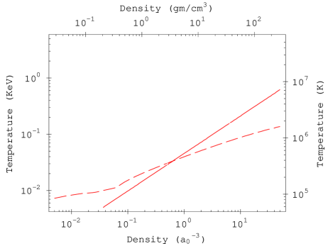
Figure 1: Region of validity of the effective theory for the case of a pure $Z=1$ ionized hydrogen plasma. On the bottom axis, density denotes the total particle density (electrons plus protons) in units of the Bohr radius, while the top axis shows the corresponding mass density. The solid line shows where the fugacity expansion breaks down. The dashed line shows where the size of “non-trivial” effective field theory corrections to the equation of state first exceed unity. (See the text for more precise descriptions.) The effective field theory is valid only in the region above both of these lines.

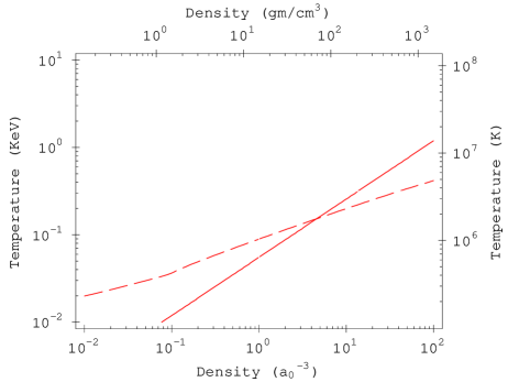
Figure 2: Region of validity for the effective theory for a pure $Z=2$ ionized helium plasma. The curves have the same meaning as in Fig. 1.

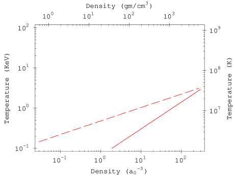
Figure 3: Region of validity for the effective theory for a pure $Z=6$ ionized carbon plasma. The curves have the same meaning as in Fig. 1.

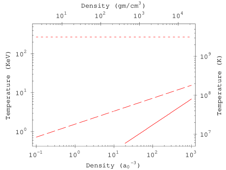
Figure 4: Region of validity for the effective theory for a pure $Z=13$ ionized aluminum plasma. The solid and dashed curves have the same meaning as in Fig. 1. The dotted horizontal line shows where relativistic corrections to the electron pressure exceed unity; our non-relativistic treatment is valid only below this line.

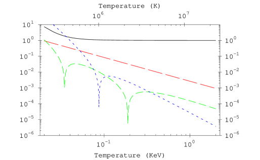
Figure 5: Corrections to the equation of state, $\beta p/n$, as a function of temperature for a pure $Z=1$ plasma with a total density (electrons plus protons) of $1\>a_{0}^{-3}$. Here, and in the following related figures, the solid line shows the ideal gas result, including quantum statistics for the electrons but no interactions. The long dashed line shows the one-loop Debye screening correction, the medium dashed line shows the two-loop correction (minus its non-interacting quantum statistics piece), and the short dashed line shows the three-loop effective field theory correction. The absolute values of the various corrections are plotted. On the two- and three-loop curves, the “cusps” pointing downward show where these corrections cross zero and change sign. For this density, the effective field theory is only useful for temperatures above about 0.06 KeV. Below this temperature, the three-loop correction exceeds the size of the one-loop correction (and exceeds unity at temperatures below about 0.04 KeV), clearly showing that the perturbative expansion of the effective theory has ceased to be reliable.

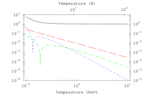
Figure 6: Same as Fig. 5, but at a total particle density of $10\>a_{0}^{-3}$.

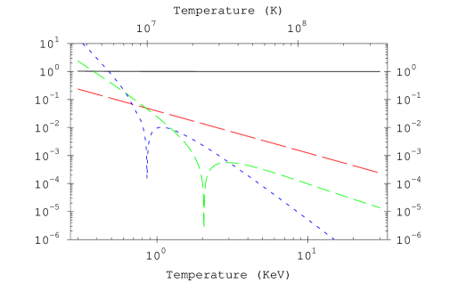
Figure 7: Same as Fig. 5, but for a pure $Z=6$ plasma at a particle density of $1\>a_{0}^{-3}$.

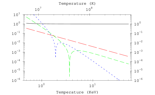
Figure 8: Same as Fig. 5, but for a pure $Z=6$ plasma at a particle density of $10\>a_{0}^{-3}$.

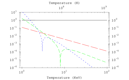
Figure 9: Same as Fig. 5, but for a pure $Z=13$ plasma at a particle density of $1\>a_{0}^{-3}$.

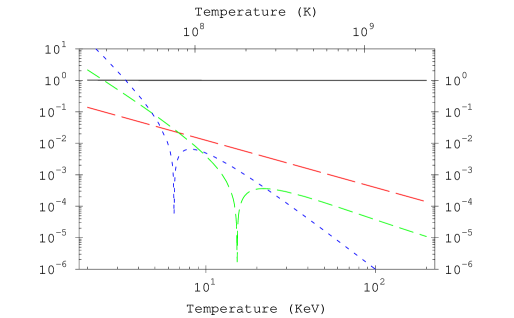
Figure 10: Same as Fig. 5, but for a pure $Z=13$ plasma at a particle density of $10\>a_{0}^{-3}$.

2 Classical Coulomb Plasmas

We consider a plasma of $A$ different species of charged particles (ions and electrons) and use the letters $a,b,\cdots=1,\cdots,A$ to denote a specific species with charge $e_{a}$ and mass $m_{a}$. In the classical limit, the particle mass only appears in the thermal wavelength

$$\lambda_{a}^{2}={2\pi\beta\hbar^{2}\over m_{a}}\,,$$ (2.1)

where $\beta$ is the inverse temperature measured in energy units, and the thermal wavelength itself only serves to define the free-particle density $n^{0}_{a}$ in terms of the chemical potential $\mu_{a}$ and spin degeneracy factor $g_{a}$ of the given species:

$$n^{0}_{a}=g_{a}\,\lambda_{a}^{-3}\,e^{\beta\mu_{a}}\,.$$ (2.2)

The grand canonical partition function for a free gas composed of these species is given by

$$Z_{\rm free}=\sum_{\{N_{a}\}}\int d\sigma_{1}^{N_{1}}\cdots d\sigma_{A}^{N_{A}}\,,$$ (2.3)

where $d\sigma_{a}^{N}$ is the $N$-particle measure for species $a$,

$$d\sigma_{a}^{N}\equiv{1\over N!}\>(d^{3}r_{a,1})\>n^{0}_{a}\cdots(d^{3}r_{a,N})\>n^{0}_{a}\,.$$ (2.4)

The factors of $\lambda_{a}^{-3}$ hidden in the $n^{0}_{a}$ free-particle densities in this measure come from performing the momentum integrals in the equilibrium phase-space distribution,

$$\lambda_{a}^{-3}=\int{(d^{3}p)\over(2\pi\hbar)^{3}}\>\exp\{-\beta p^{2}/2m_{a}\}\,,$$ (2.5)

and the remaining parts of $n^{0}_{a}$ arise from the degeneracy ($g_{a}$) and fugacity ($e^{\beta\mu_{a}}$) factors that enter into the definition of the grand canonical ensemble. Introducing the total volume of the system

$${\cal V}\equiv\int(d^{3}{\bf r})\,,$$ (2.6)

which we shall always assume is arbitrarily large, and carrying out the summations, we get

$$Z_{\rm free}=\prod_{a=1}^{A}\>\sum_{N_{a}}{({\cal V}\,n^{0}_{a})^{N_{a}}\over N_{a}!}=\exp\biggl{\{}{\cal V}\sum_{a=1}^{A}\>n^{0}_{a}\biggr{\}}\,.$$ (2.7)

2.1 Functional Integral for the Classical Partition Function

The corresponding grand canonical partition function for a plasma with Coulomb interactions between all the charged particles is

$$Z=\sum_{\{N_{a}\}}\int d\sigma_{1}^{N_{1}}\cdots d\sigma_{A}^{N_{A}}\>\exp\biggl{\{}-{\beta\over 2}\,\sum_{k\neq l}e_{k}e_{l}\,V_{C}\left({\bf r}_{k}{-}{\bf r}_{l}\right)\biggr{\}}\,.$$ (2.8)

Here the indices $k\,,l$ in the exponential run over all particles of all the various types; ${\bf r}_{k}$ and $e_{k}$ denote the coordinates and charge of any given particle, respectively. We employ rational units, so that the Coulomb potential for unit charges is given by

$$V_{C}({\bf r})={1\over 4\pi\,r}\,.$$ (2.9)

We choose to work with the grand canonical ensemble because, as we shall see, it has a simple functional integral representation which leads to a very convenient diagrammatic form for perturbation theory and allows easy use of effective field theory techniques. However, we are ultimately interested in calculating physical quantities as a function of the particle densities, not chemical potentials, of the various species. Since the presence of interactions between particles will modify the particle density — chemical potential relation, we will need to compute particle densities as a function of chemical potential, and then invert this relation (order-by-order in perturbation theory) to re-express results in terms of particle densities. The physical particle densities, which we will denote as $\bar{n}_{a}$, satisfy charge neutrality,

$$\langle Q\rangle_{\beta}={\cal V}\,\sum_{a}\>e_{a}\,\bar{n}_{a}=0\,,$$ (2.10)

as required for a sensible thermodynamic limit.

It will be useful to regard the chemical potentials as temporarily having arbitrary spatial variation, $\mu_{a}(\bf r)$. This extends the partition function to be a functional of these generalized chemical potentials, $Z\to Z[\mu]$, which is then the generating functional for number density correlation functions. The free-particle number density — chemical potential relation (2.2) is now generalized to

$$n^{0}_{a}({\bf r})\equiv g_{a}\,\lambda_{a}^{-3}\,e^{\beta\mu_{a}({\bf r})}\,,$$ (2.11)

with the variational derivative

$${\delta\over\delta\beta\mu_{b}({\bf r}^{\prime})}\,n^{0}_{a}({\bf r})=\delta_{ab}\,\delta({\bf r}{-}{\bf r}^{\prime})\,n^{0}_{a}({\bf r})\,.$$ (2.12)

Here, and henceforth, variations in $\beta\mu_{a}$, and in $\beta$, will be regarded as independent. In other words, $\beta\mu_{a}$ is to be varied while holding $\beta$ fixed, and vice-versa. The density of particles of species $a$ is given by the variational derivative of $\ln Z[\mu]$ with respect to the corresponding generalized chemical potential,

$$\left\langle n_{a}({\bf r})\right\rangle_{\beta}\equiv\left\langle{\sum}_{i}\>\delta({\bf r}{-}{\bf r}_{a,i})\right\rangle_{\beta}={\delta\over\delta\beta\mu_{a}({\bf r})}\ln Z[\mu]\,,$$ (2.13)

while two functional derivatives yield the connected part of the density-density correlator,

$$K_{ab}({\bf r}{-}{\bf r}^{\prime}) \equiv \left\langle n_{a}({\bf r})\>n_{b}({\bf r}^{\prime})\right\rangle_{\beta}-\left\langle n_{a}({\bf r})\right\rangle_{\beta}\left\langle n_{b}({\bf r}^{\prime})\right\rangle_{\beta}$$ (2.14)

$$= \left\langle{\sum}_{i,j}\delta({\bf r}{-}{\bf r}_{a,i})\>\delta({\bf r}^{\prime}{-}{\bf r}_{b,j})\right\rangle_{\beta}-\left\langle{\sum}_{i}\delta({\bf r}{-}{\bf r}_{a,i})\right\rangle_{\beta}\left\langle{\sum}_{j}\delta({\bf r}^{\prime}{-}{\bf r}_{b,j})\right\rangle_{\beta}$$

$$= {\delta\over\delta\beta\mu_{a}({\bf r})}\,{\delta\over\delta\beta\mu_{b}({\bf r}^{\prime})}\,\ln Z[\mu]\,.$$

After the functional derivatives have been taken, it will be assumed that the spatially-dependent, generalized chemical potentials $\mu_{c}({\bf r})$ revert to the usual constant chemical potentials $\mu_{c}$.

The cumbersome form of the grand partition functional (2.8) can be replaced by a much leaner functional integral representation by using the Gaussian integral relation

$$\int[d\phi]\exp\left\{\beta\int(d^{\nu}{\bf r})\left[{\textstyle{1\over 2}}\,\phi({\bf r})\nabla^{2}\phi({\bf r})+i\rho({\bf r})\phi({\bf r})\right]\right\}$$

$$\qquad\qquad={\rm Det}^{-1/2}\left[\beta(-\nabla^{2})\right]\exp\left\{-{\beta\over 2}\int(d^{\nu}{\bf r})(d^{\nu}{\bf r}^{\prime})\>\rho({\bf r})\,V_{\nu}({\bf r}{-}{\bf r}^{\prime})\,\rho({\bf r}^{\prime})\right\},$$ (2.15)

which follows from completing the square in the functional integral on the left. The auxiliary field $\phi({\bf r})$ is nothing but the electrostatic scalar potential. The relation above has been written in $\nu$ spatial dimensions with

$$V_{\nu}({\bf r}{-}{\bf r}^{\prime})\equiv\int{(d^{\nu}{\bf k})\over(2\pi)^{\nu}}\>{e^{i{\bf k}\cdot({\bf r}{-}{\bf r}^{\prime})}\over{\bf k}^{2}}$$ (2.16)

the Coulomb potential in $\nu$ dimensions. We choose to make a continuation in spatial dimensions at this juncture because it automatically removes infinite particle self-interactions. Dimensional continuation is a regularization procedure which introduces no external or extraneous dimensional constants. Hence, since there is nothing available to make up the correct dimensional quantity, in dimensional continuation

$$V_{\nu}({\bf 0})=0\,,$$ (2.17)

and particle self-interactions vanish. We shall see how this works out in practice as our development unfolds. We shall also need the technique of dimensional continuation to deal with the short-distance divergences of the classical Coulomb theory — the divergences that are removed by quantum fluctuations which we shall later handle using effective field theory methods. Hence one might as well get accustomed to dimensional continuation at an early stage. At the end of our computations we shall, of course, take $\nu\to 3$. In view of the functional formula (2.15), it follows that the grand canonical partition function may be written as

$$Z[\mu] = {\rm Det}^{1/2}\left[\beta(-\nabla^{2})\right]\int[d\phi]\,\exp\left\{-{\beta\over 2}\int(d^{\nu}{\bf r})\>\phi({\bf r})\left(-\nabla^{2}\right)\phi({\bf r})\right\}$$ (2.18)

$$\kern 104.79128pt{}\times\exp\left\{\sum_{a=1}^{A}\int(d^{\nu}{\bf r})\>n^{0}_{a}({\bf r})\>e^{i\beta e_{a}\phi({\bf r})}\right\}.$$

Since $-\nabla^{2}$ is a positive operator, the first, Gaussian, part of the integrand gives a well-defined and convergent functional integral. Expanding the second exponential in a power series in the free-particle densities $n^{0}_{a}$, and using the functional integration formula (2.15), it is easy to see that the result (2.18) does indeed reproduce the Coulomb plasma generating functional (2.8). Note that this equivalence requires that the self-interaction terms vanish, which is the case with our dimensional regularization [Eq. (2.17)]. Combining the two exponentials of (2.18), one may write the partition function in the concise form

$$Z[\mu]=N_{0}\int[d\phi]\,e^{-S_{\rm cl}[\phi;\mu]}\,,$$ (2.19)

with an “action” functional defined by

$$S_{\rm cl}[\phi;\mu]\equiv\int(d^{\nu}{\bf r})\>\left\{{\beta\over 2}\left[\nabla\phi({\bf r})\right]^{2}-\sum_{a=1}^{A}n^{0}_{a}({\bf r})\>e^{i\beta e_{a}\phi({\bf r})}\right\},$$ (2.20)

and the overall normalization factor

$$N_{0}\equiv{\rm Det}^{1/2}\left[\beta(-\nabla^{2})\right].$$ (2.21)

Varying the functional integral representation (2.19) with respect to the chemical potential $\mu_{a}({\bf r})$ yields the representation

$$\left\langle n_{a}({\bf r})\right\rangle_{\beta}=\left<\!\!\left<n^{0}_{a}({\bf r})\,e^{i\beta e_{a}\phi({\bf r})}\right>\!\!\right>$$ (2.22)

for the density of particles of type $a$, where in general $\left<\!\left<\cdots\right>\!\right>$ denotes a functional integral average,

$$\left<\!\left<{\cal O}\right>\!\right>\equiv Z[\mu]^{-1}\>N_{0}\int[d\phi]\>e^{-S_{\rm cl}[\phi]}\>{\cal O}\,.$$ (2.23)

With the generalized chemical potentials restricted to constant values, Eq. (2.22) gives the functional integral representation for the usual grand canonical average of the number density of particles of species $a$. A second variation with the chemical potentials then restricted to constant values yields the representation of the density-density correlation function (2.14),

$$K_{ab}({\bf r}{-}{\bf r}^{\prime}) = \left<\!\!\left<n^{0}_{a}\,e^{i\beta e_{a}\phi({\bf r})}\>n^{0}_{b}\,e^{i\beta e_{b}\phi({\bf r}^{\prime})}\right>\!\!\right>-\left<\!\!\left<n^{0}_{a}\,e^{i\beta e_{a}\phi({\bf r})}\right>\!\!\right>\left<\!\!\left<n^{0}_{b}\,e^{i\beta e_{b}\phi({\bf r}^{\prime})}\right>\!\!\right>$$ (2.24)

$$\quad{}+\delta_{ab}\,\delta({\bf r}{-}{\bf r}^{\prime})\left<\!\!\left<n^{0}_{a}\,e^{i\beta e_{a}\phi({\bf r})}\>\right>\!\!\right>\,.$$

The final contact term proportional to $\delta({\bf r}{-}{\bf r}^{\prime})$ appears (when $a=b$) because the functional integral naturally generates correlators involving distinct particles,

$$\left<\!\!\left<n^{0}_{a}\,e^{i\beta e_{a}\phi({\bf r})}\>n^{0}_{a}\,e^{i\beta e_{a}\phi({\bf r}^{\prime})}\right>\!\!\right>=\left\langle{\sum}_{i\neq j}\>\delta({\bf r}{-}{\bf r}_{a,i})\,\delta({\bf r}^{\prime}{-}{\bf r}_{a,j})\right\rangle_{\beta}\,.$$ (2.25)

This differs from the corresponding term in (2.14) precisely by the single-particle contact term $\left\langle{\sum}_{i}\delta({\bf r}{-}{\bf r}_{a,i})\,\delta({\bf r}^{\prime}{-}{\bf r}_{a,i})\right\rangle_{\beta}=\delta({\bf r}{-}{\bf r}^{\prime})\,\left\langle n_{a}\right\rangle_{\beta}$.

Since the functional integral of a total derivative vanishes,

$$0=\int[d\phi]\>{\delta\over\delta\phi({\bf r})}\,e^{-S_{\rm cl}[\phi;\mu]}\,,$$ (2.26)

the field equation $\left<\!\left<\delta S_{\rm cl}[\phi;\mu]/\delta\phi({\bf r})\right>\!\right>=0$ is an exact identity. For the action (2.20), this is the Poisson equation

$$\nabla^{2}\left<\!\left<i\phi({\bf r})\right>\!\right>=\left<\!\left<\rho({\bf r})\right>\!\right>$$ (2.27)

with the charge density

$$\rho({\bf r})\equiv\sum_{a=1}^{A}\>e_{a}\,n^{0}_{a}({\bf r})\,e^{i\beta e_{a}\phi({\bf r})}\,.$$ (2.28)

Integrating both sides of (2.27) over all space yields the condition of total charge neutrality,

$$0=\left\langle Q\right\rangle_{\beta}=\sum_{a=1}^{A}e_{a}\int(d^{\nu}{\bf r})\>\left\langle n_{a}({\bf r})\right\rangle_{\beta}\,.$$ (2.29)

This identity holds for any choice of the generalized chemical potentials $\mu_{a}({\bf r})$, in essence because the average value of the electrostatic potential $\phi$ will always adjust itself to produce a charge neutral equilibrium state.

The fact that the chemical potentials enter the action (2.20) only through the combination $n^{0}_{a}e^{i\beta e_{a}\phi}$ (with $n^{0}_{a}\propto e^{\beta\mu_{a}}$) means that the theory is completely unchanged if the electrostatic potential is shifted by an arbitrary constant,

$$i\phi\to i\phi+c\,,$$ (2.30)

provided the chemical potentials are correspondingly adjusted,

$$\mu_{a}\to\mu_{a}-e_{a}\,c\,.$$ (2.31)

Consequently, the values of the chemical potentials are not uniquely determined by the physical particle densities. This is also reflected in the fact that the conditions

$$\bar{n}_{a}=\left\langle n_{a}\right\rangle_{\beta}\,,\qquad a=1,\ldots,A\,,$$ (2.32)

only give $A-1$ linearly independent constraints on the chemical potentials — precisely because charge neutrality (2.29) is an automatic identity. To obtain uniquely defined chemical potentials (when they revert back to their normal constant values), one must remove the (physically irrelevant) freedom (2.30)–(2.31) to shift the mean value of the electrostatic potential. We will make the obvious choice, and demand that the thermal average of the electrostatic potential vanish,

$$\left<\!\left<\phi\right>\!\right>\equiv 0\,,$$ (2.33)

to fix the chemical potentials uniquely.

2.2 Mean Field Theory

Saddle-points of the functional integral (2.19) correspond to solutions of the field equation

$${\delta S_{\rm cl}[\phi;\mu]\over\delta\phi({\bf r})}=0\,,$$ (2.34)

which, for the action (2.20), is just the Debye-Hückel equation

$$-\nabla^{2}\phi({\bf r})=i\sum_{a=1}^{A}\>e_{a}\,n^{0}_{a}({\bf r})\,e^{i\beta e_{a}\phi({\bf r})}\,.$$ (2.35)

The leading saddle-point approximation corresponds to neglecting all fluctuations in $\phi$ away from the saddle-point, so that

$$\ln Z_{0}[\mu]=-S_{\rm cl}[\phi;\mu]\,,$$ (2.36)

with $\phi$ solving the field equation (2.35). In quantum field theory, this approximation is commonly called the tree approximation because the classical action is the generating functional of connected tree graphs. In statistical mechanics it is known as the mean field approximation. In Appendix A we shall describe the effective action functional $\Gamma[\phi;\mu]$ which is the generalization of the classical action $S_{\rm cl}[\phi;\mu]$ that takes account of the thermal fluctuations about the mean field which are described by the functional integral and thus provides an exact description of the plasma. As will be shown in Appendix A, the effective action method can be used to derive general properties of the plasma physics. Our work now with the mean field approximation will provide an introduction to the later use of the more general effective action as well as illustrating basic plasma properties.

For constant chemical potentials, the field equation reduces to the (lowest-order) charge neutrality condition,

$$\sum_{a}e_{a}\,n^{0}_{a}\,e^{ie_{a}\beta\phi}=0\,,$$ (2.37)

and

$$\ln Z_{0}[\mu]={\cal V}\sum_{a}\>n^{0}_{a}\,e^{ie_{a}\beta\phi}\,.$$ (2.38)

The mean-field number density — chemical potential relation is given by

$$\bar{n}_{a} = {\cal V}^{-1}\>\left.{\partial\ln Z_{0}\over\partial\beta\mu_{a}}\right|_{\beta}$$ (2.39)

$$= n^{0}_{a}\,e^{ie_{a}\beta\phi}+i\beta\left[\sum_{a}e_{a}n^{0}_{a}e^{ie_{a}\beta\phi}\right]{\partial\phi\over\partial\beta\mu_{a}}$$

$$= n^{0}_{a}\,e^{ie_{a}\beta\phi}\,,$$

with the last equality following from the charge neutrality condition (2.37). If the free-particle densities satisfy “bare” charge neutrality,

$$0=\sum_{a}e_{a}\,n^{0}_{a}\,,$$ (2.40)

then the saddle-point condition (2.37) has the trivial solution $\phi({\bf r})=0$, the physical densities $\bar{n}_{a}$, within this mean field approximation, will equal the free-particle densities $n^{0}_{a}$, and the mean-field partition function equals the usual ideal gas result,

$$Z_{0}=\exp\biggl{\{}{\cal V}\sum_{a=1}^{A}n^{0}_{a}\biggr{\}}\,.$$ (2.41)

The average energy of our grand canonical ensemble is the thermodynamic internal energy,

$$U=\bar{E}=\langle E\rangle_{\beta}=-\left.{\partial\ln Z\over\partial\beta}\right|_{\beta\mu}\,.$$ (2.42)

Since $n^{0}_{a}\sim\beta^{-3/2}$, varying the neutrality condition (2.37) with respect to $\beta$ gives

$$-{3\over 2}\,\beta^{-1}\sum_{a}e_{a}\,n^{0}_{a}\,e^{ie_{a}\beta\phi}+{i\over\beta}\,\kappa_{0}^{2}\,{\partial(\beta\phi)\over\partial\beta}=0\,,$$ (2.43)

where

$$\kappa_{0}^{2}\equiv\sum_{a}\beta\,e^{2}_{a}\,n^{0}_{a}\,e^{ie_{a}\beta\phi}$$ (2.44)

will be seen to be the lowest-order (squared) Debye wave number. The first term of (2.43) again vanishes by virtue of charge neutrality (2.37), and so

$${\partial(\beta\phi)\over\partial\beta}=0\,.$$ (2.45)

Hence, to lowest order the average energy

$$\bar{E}={3\over 2}\,\beta^{-1}{\cal V}\,\sum_{a}\bar{n}_{a}={3\over 2}\,T\,\sum_{a}\bar{N}_{a}\,,$$ (2.46)

which is just the familiar formula for an ideal gas.

Second derivatives of $\ln Z$ produce correlators. The second derivative of $\ln Z_{0}$ with respect to the inverse temperature gives the lowest-order result for the mean square fluctuation in energy,

$$\left\langle\left(E-\bar{E}\right)^{2}\right\rangle_{\beta}=-{\partial\bar{E}\over\partial\beta}={15\over 4}\,T\bar{E}\,.$$ (2.47)

Mixed temperature — chemical potential derivatives yield the correlation between energy and particle number fluctuations,

$$\left\langle\left(E-\bar{E}\right)\left(N_{a}-\bar{N}_{a}\right)\right\rangle_{\beta}=-{\partial\bar{N}_{a}\over\partial\beta}={3\over 2}\,T\,\bar{N}_{a}\,.$$ (2.48)

These are again just the results for a free gas. But for fluctuations in particle numbers, given by second derivatives with respect to the chemical potentials, one must account for the fact that varying the chemical potentials will cause the mean field to vary. Since the charge neutrality constraint (2.37) holds for arbitrary chemical potentials, varying it with respect to the chemical potentials yields

$$e_{a}\,\bar{n}_{a}+i\,\kappa_{0}^{2}\,{\partial\phi\over\partial\beta\mu_{a}}=0\,,$$ (2.49)

Hence,

$$\left\langle\left(N_{a}-\bar{N}_{a}\right)\left(N_{b}-\bar{N}_{b}\right)\right\rangle_{\beta}={\partial N_{a}\over\partial\beta\mu_{b}} = \delta_{ab}\bar{N}_{a}+\bar{N}_{a}ie_{a}\,\beta\,{\partial\phi\over\partial\beta\mu_{b}}$$ (2.50)

$$= \delta_{ab}\bar{N}_{a}-e_{a}\bar{N}_{a}{\beta\over\kappa_{0}^{2}}\,e_{b}\,\bar{n}_{b}\,.$$

The physical implications of this result, which differs from the ideal gas result, will be discussed below in subsection 2.7.

2.3 Loop Expansion

The saddle-point (or “loop”) expansion of the functional integral (2.19), incorporates corrections beyond mean field theory and systematically generates the perturbative expansion for physical quantities of interest. In the development that follows, we shall assume that all of the desired functional derivatives with respect to the generalized, spatially varying chemical potentials which produce the insertions in the functional integral, as shown in the previous number density (2.22) and density-density correlator (2.24), have already been taken. Thus, we henceforth restrict our considerations to constant chemical potentials. In the lowest-order approximation, the free-particle densities $n^{0}_{a}$ will equal the physical densities $\bar{n}_{a}$, which are charge neutral (2.10). However, perturbative corrections to the chemical potential — number density relation will shift the free-particle densities away from the physical densities, and therefore displace the true saddle point away from $\phi=0$. Even though the bare neutrality constraint (2.40) no longer holds in higher orders, it will be most convenient to expand the functional integral about $\phi=0$ instead of the true saddle-point value. At each stage of this (loop) expansion, further corrections to the bare (tree approximation) charge neutrality constraint (2.40) appear which alter the relation amongst the chemical potentials that arises from charge neutrality. Expanding the action in powers of $\phi$ and separating the quadratic and constant terms gives

$$S_{\rm cl}[\phi;\mu]=S_{0}[\phi;\mu]+\Delta S[\phi;\mu]\,,$$ (2.51)

where

$$S_{0}[\phi;\mu]\equiv\int(d^{\nu}{\bf r})\>\biggl{\{}-\sum_{a=1}^{A}n^{0}_{a}+{\beta\over 2}\,\phi({\bf r})\left[-\nabla^{2}+\kappa_{0}^{2}\right]\phi({\bf r})\biggr{\}}\,,$$ (2.52)

and

$$\Delta S[\phi;\mu] \equiv -\int(d^{\nu}{\bf r})\>\sum_{a=1}^{A}n^{0}_{a}\left\{e^{i\beta e_{a}\phi({\bf r})}-1+{\textstyle{1\over 2}}\beta^{2}e_{a}^{2}\phi({\bf r})^{2}\right\}$$ (2.53)

$$= -\int(d^{\nu}{\bf r})\>\sum_{a=1}^{A}n^{0}_{a}\left\{[i\beta e_{a}\phi({\bf r})]+{\textstyle{1\over 3!}}[i\beta e_{a}\phi({\bf r})]^{3}+{\textstyle{1\over 4!}}[i\beta e_{a}\phi({\bf r})]^{4}+\cdots\right\}.$$

In Eq. (2.52), $\kappa_{0}^{2}$ is the lowest-order Debye wave number previously defined in Eq. (2.44). Since the bare neutrality condition is modified by loop corrections, $\sum_{a}e_{a}n^{0}_{a}$ will not vanish beyond the mean field approximation. Consequently, $\Delta S$ contains a piece linear in the field $\phi$ and $\phi=0$ does not remain a saddle point in higher orders.

Evaluating the action at $\phi=0$ gives the ideal gas partition function The first (“one-loop”) correction is obtained by neglecting $\Delta S$ and integrating over fluctuations in $\phi$ with just the quadratic action $S_{0}$. This gives the Gaussian functional integral

$$Z_{1} = Z_{0}\>{\rm Det}^{1/2}\left[\beta(-\nabla^{2})\right]\int[d\phi]\,\exp\left\{-{\beta\over 2}\int(d^{\nu}{\bf r})\>\phi({\bf r})\left(-\nabla^{2}+\kappa_{0}^{2}\right)\phi({\bf r})\right\}$$ (2.54)

$$= Z_{0}\>{\rm Det}^{-1/2}\left[1+{1\over-\nabla^{2}}\,\kappa_{0}^{2}\right]\,.$$

The product of the determinant produced by the Gaussian integration with the prefactor (which may be written as the inverse determinant of the operator inverse) produces the determinant shown on the second line. This functional determinant will be evaluated shortly. The correlation function of potential fluctuations $\left<\!\left<\phi({\bf r})\phi({\bf r}^{\prime})\right>\!\right>$, to lowest order, is given by the Green’s function for the linear operator $\left(-\nabla^{2}+\kappa_{0}^{2}\right)$ appearing in $S_{0}$,

$$\beta\left<\!\left<\phi({\bf r})\phi({\bf r}^{\prime})\right>\!\right>^{(0)}={N_{0}\over Z_{1}}\int[d\phi]\>e^{-S_{0}}\>\beta\phi({\bf r})\phi({\bf r}^{\prime})=G_{\nu}({\bf r}{-}{\bf r}^{\prime})\,.$$ (2.55)

Here $G_{\nu}({\bf r}{-}{\bf r}^{\prime})$ denotes the Debye Green’s function (in $\nu$-dimensions), which satisfies

$$\left[-\nabla^{2}+\kappa^{2}_{0}\,\right]G_{\nu}({\bf r}{-}{\bf r}^{\prime})=\delta({\bf r}{-}{\bf r}^{\prime})\,,$$ (2.56)

and has the Fourier representation

$$G_{\nu}({\bf r}{-}{\bf r}^{\prime})=\int{(d^{\nu}{\bf k})\over(2\pi)^{\nu}}\>{e^{i{\bf k}\cdot({\bf r}{-}{\bf r}^{\prime})}\over{\bf k}^{2}+\kappa_{0}^{2}}\,.$$ (2.57)

Expanding the functional integral (2.19) in powers of $\Delta S$ will lead to Feynman diagrams in which each line represents a factor of this Debye Green’s function times $1/\beta$, with vertices joining $k$ lines representing factors of $\sum_{a}n^{0}_{a}\,(i\beta e_{a})^{k}$.

A convenient integral representation for the Debye Green’s function in a space of arbitrary dimensions is obtained by writing the denominator in (2.57) as a parameter integral of an exponential, interchanging the parameter and wave number integrals, and completing the square to perform the wave number integral:

$$G_{\nu}({\bf r})=\int_{0}^{\infty}ds\>e^{-\kappa_{0}^{2}s}\int{(d^{\nu}{\bf k})\over(2\pi)^{\nu}}\>e^{-{\bf k}^{2}s}e^{i{\bf k}\cdot{\bf r}}=\int_{0}^{\infty}ds\>\left(4\pi s\right)^{-\nu/2}\,e^{-\kappa_{0}^{2}s-({\bf r}^{2}/4s)}\,.$$ (2.58)

The coincident limit of the Debye Green’s function $G_{\nu}({\bf 0})$ will be needed in the following sections. In this limit, the representation (2.58) becomes the standard representation of the Gamma function, and we have

$$G_{\nu}({\bf 0})={\kappa_{0}^{\nu-2}\over(4\pi)^{\nu/2}}\,\Gamma\left(1{-}{\nu\over 2}\right)\,.$$ (2.59)

Since $\Gamma(-{\textstyle{1\over 2}})=-2\sqrt{\pi}$, the $\nu\to 3$ limit of $G_{\nu}({\bf 0})$ is perfectly finite and yields

$$\lim_{\nu\to 3}G_{\nu}({\bf 0})=-{\kappa_{0}\over 4\pi}\,.$$ (2.60)

Comparing this with the Debye Green’s function fixed at three dimensions,

$$G_{3}({\bf r})={e^{-\kappa_{0}r}\over 4\pi r}\,,$$ (2.61)

one sees that

$$\lim_{r\to 0}{1\over 4\pi r}\left[e^{-\kappa_{0}r}-1\right]=-{\kappa_{0}\over 4\pi}\,.$$ (2.62)

In other words, the dimensional regularization method automatically deletes the vacuum self-energy contribution that comes from the pure Coulomb potential.

2.4 Particle Densities

Although the densities of the various particle species may be obtained simply by differentiating the partition function with respect to the corresponding chemical potential — which we shall do subsequently — one may directly evaluate these densities using diagrammatic perturbation theory. We shall do this through one-loop order to illustrate the working of the perturbation theory and charge neutrality. In perturbation theory, the density of particles of a given species is evaluated by expanding the exponential in (2.22) in powers of $\phi$ yielding, to one loop order,

$$\left\langle n_{a}\right\rangle_{\beta}^{(1)} = \left<\!\left<n^{0}_{a}\,e^{i\beta e_{a}\phi({\bf r})}\right>\!\right>$$ (2.63)

$$= n^{0}_{a}\left[1+i\beta e_{a}\left<\!\left<\phi({\bf r})\right>\!\right>-{\textstyle{1\over 2}}\beta^{2}e_{a}^{2}\left<\!\left<\phi({\bf r})^{2}\right>\!\right>\right]$$

$$= n^{0}_{a}\left[1+i\beta e_{a}\left<\!\left<\phi\right>\!\right>^{(1)}-{\textstyle{1\over 2}}\beta\,e_{a}^{2}\,G_{\nu}({\bf 0})\right].$$

In the tree approximation with $\phi=0$, the charge neutrality condition (2.37) requires that the chemical potentials are arranged such that $\sum e_{a}\,n^{0}_{a}=0$. Thus, this sum should be considered to start out at one-loop order. The one-legged vertex, the coefficient of the term in the interaction part of the action (2.53) linear in $\phi$, is proportional to this sum, and hence it also should be considered to start at one-loop order. Thus computing the expectation value of $\phi$ to one-loop order requires expanding $e^{-\Delta S}$ in powers of $\phi$ and keeping the linear and cubic terms. This expansion, shown in the graphs of figure 11, gives

$$\left<\!\left<\phi\right>\!\right>^{(1)} = {N_{0}\over Z_{1}}\int[d\phi]\>e^{-S_{0}}\>\phi({\bf 0})\int(d^{\nu}{\bf r})\>\sum_{a}n^{0}_{a}\left[(i\beta e_{a}\phi({\bf r}))+{\textstyle{1\over 3!}}(i\beta e_{a}\phi({\bf r}))^{3}\right]$$ (2.64)

$$= {i\over\kappa_{0}^{2}}\>\sum_{a=1}^{A}\>e_{a}\,n^{0}_{a}\left[1-{\textstyle{1\over 2}}\beta\,e_{a}^{2}\,G_{\nu}({\bf 0})\right].$$

This calculation is spelled out in greater detail in the derivation of Eq. (F.21) in Appendix F. Note that the first term in Eq. (2.64), the tree approximation, is obtained by expanding the tree level neutrality condition (2.37) to zeroth and first order in $\phi$.

Figure 11: One-loop order contributions to $\left\langle\phi\right\rangle_{\beta}$. Unlabeled blobs (or vertices) represent insertions of $-\Delta S$ taken to some order in $\phi$; a vertex joining $k$ lines stands for a factor of $\sum_{a}n^{0}_{a}\,(i\beta e_{a})^{k}$. Each line represents a factor of the Debye Green’s function divided by $\beta$, and the contribution of each diagram is to be multiplied by the appropriate symmetry factor which, for the diagram above containing a loop, the “tadpole graph,” is $1/2$. [The basic rules for diagrammatic perturbation theory, corresponding to a saddle-point expansion of the functional integral, are discussed in virtually all textbooks on quantum field theory. See, for example, Refs. [23, 25, 26].] The condition $\left<\!\left<\phi\right>\!\right>=0$ taken to one-loop order implies that the one-legged vertex (—$\bullet$) must cancel the one-loop “tadpole”. Hence this one-legged vertex should be counted here as being a one-loop contribution. Two-loop diagrams (and beyond) generate further higher-order corrections to the one-legged vertex $i\beta{\sum}_{a}e_{a}\,n_{a}^{0}$.

Figure 12: One-loop order contributions to the mean particle density $\left\langle n_{a}\right\rangle_{\beta}$. Labeled blobs (${}_{a}\bullet$) refer to insertions of the number density $n^{0}_{a}\,e^{i\beta e_{a}\phi}$ for a given species; a labeled blob radiating $k$ lines stands for a factor of $n^{0}_{a}\,(i\beta e_{a})^{k}$. The condition $\left<\!\left<\phi\right>\!\right>=0$ implies that the second and third diagrams cancel. More generally, the condition $\left<\!\left<\phi\right>\!\right>=0$ implies that such “tadpole” diagrams cancel in the expansion of any quantity, and such diagrams may simply be neglected. This cancelation is described more fully in Appendix A.

Imposing the condition (2.33) that the mean electrostatic potential vanish now requires, to this order, that

$$\sum_{a=1}^{A}\>e_{a}\,n^{0}_{a}={\textstyle{1\over 2}}\beta\,G_{\nu}({\bf 0})\sum_{a=1}^{A}e_{a}^{3}\,n^{0}_{a}\,,$$ (2.65)

which alters the tree level neutrality constraint (2.40) on the chemical potentials, making the sum on the left-hand side of Eq (2.65) equal to the one-loop contribution on the right-hand side. This confirms the statement above that the sum on the left-hand should be considered to start out at one-loop order. With the imposition of the one-loop constraint (2.65), the expression (2.63) for the one-loop densities simplifies to

$$\left\langle n_{a}\right\rangle_{\beta}^{(1)}=n^{0}_{a}\left[1-{\textstyle{1\over 2}}\beta\,e_{a}^{2}\,G_{\nu}({\bf 0})\right].$$ (2.66)

The discussion of the density that we have just given is illustrated in figure 12. Inverting the one-loop density relation (2.66) to express the bare density $n^{0}_{a}$ in terms of the physical density $\bar{n}_{a}$ gives

$$n^{0}_{a}=\bar{n}_{a}\left[1-{\textstyle{1\over 2}}\beta\,e_{a}^{2}\,G_{\nu}({\bf 0})\right]^{-1}=\bar{n}_{a}\left[1+{\textstyle{1\over 2}}\beta\,e_{a}^{2}\,G_{\nu}({\bf 0})\right],$$ (2.67)

to one-loop order. Note that $e_{a}^{2}G_{\nu}({\bf 0})/2$ is the self-energy of a charge $e_{a}$ in the Debye screened plasma, and so the right-hand side of Eq. (2.66) may be recognized as the first order expansion of the Boltzmann factor $\exp\{-\beta e_{a}^{2}G_{\nu}({\bf 0})/2\}$. Other effects besides this simple exponentiation of course appear in higher orders. Also note that the mean charge density (computed to one-loop order) vanishes, as it must, even before the imposition of the constraint (2.65), for it follows from Eq’s. (2.63) and (2.64) and the definition (2.44) of the lowest-order Debye wave number that

$$\left\langle\rho\right\rangle_{\beta}^{(1)} = \sum_{b=1}^{A}\>e_{b}\left\langle n_{b}\right\rangle_{\beta}^{(1)}$$ (2.68)

$$= \sum_{b=1}^{A}\>e_{b}\,n^{0}_{b}\left[1-{\textstyle{1\over 2}}\beta\,e_{b}^{2}\,G_{\nu}({\bf 0})\right]+\sum_{b=1}^{A}\>\beta\,e_{b}^{2}\,n^{0}_{b}\>\left<\!\left<i\phi\right>\!\right>^{(1)}$$

$$= \sum_{a=1}^{A}\>e_{a}\,n^{0}_{a}\left[1-{\textstyle{1\over 2}}\beta\,e_{a}^{2}\,G_{\nu}({\bf 0})\right]\left(1-\sum_{b=1}^{A}\>{\beta\,e_{b}^{2}\,n^{0}_{b}\over\kappa_{0}^{2}}\right)$$

$$= 0\,.$$

2.5 Loop Expansion Parameter

We have just seen that the size of one-loop corrections is measured, in $\nu$ dimensions, by the dimensionless parameter $\beta e^{2}G_{\nu}({\bf 0})\sim\beta e^{2}\kappa_{0}^{\nu-2}$, which reduces to $\beta e^{2}\kappa_{0}$ in three dimensions. This parameter is the essentially the ratio of the Coulomb energy for two particles separated by a Debye screening distance to their typical kinetic energy in the plasma. Since $\kappa_{0}^{2}\sim\beta e^{2}/d^{3}$, where $d$ is the average interparticle spacing, this expansion parameter is also $[\,\beta e^{2}/d]^{3/2}$ — the $3/2$ power of the ratio of the average Coulomb energy in the plasma to the kinetic energy in the plasma.

At higher orders in the perturbative expansion, the relative contribution of any Feynman diagram containing $\ell$ loops will be suppressed by $[\,\beta e^{2}\kappa_{0}^{\nu-2}]^{\ell}$, or in three dimensions, by $[\,\beta e^{2}\kappa_{0}]^{\ell}$. A detailed proof of this appears in section 3 of Appendix F. In other words, the loop expansion parameter is $[\,\beta e^{2}\kappa_{0}]$ (up to some $O(1)$ numerical factor). In fact, we shall find in our explicit calculations that $[\beta e^{2}\kappa/4\pi]$ appears as the most natural loop expansion parameter.

2.6 Thermodynamic Quantities

All thermodynamic quantities may be derived from the grand canonical partition function. In particular, the internal energy density $u$ is given by

$$u{\cal V}=-\left.{\partial\ln Z\over\partial\beta}\right|_{\beta\mu}\,,$$ (2.69)

where, as indicated the partial derivative is taken with the all the $\beta\mu_{a}$ fixed, while the chemical potential — number density relation is given by

$$\bar{n}_{a}{\cal V}=\left.{\partial\ln Z\over\partial\beta\mu_{a}}\right|_{\beta}\,,$$ (2.70)

where now $\beta$ is held fixed in the partial differentiation. The grand potential $\Omega({\cal V},T,\{\mu_{a}\})$ is related to the partition function of the grand canonical ensemble by

$$Z=e^{-\beta\Omega}\,.$$ (2.71)

The grand potential is extensive for a macroscopic volume, and it is simply related to the pressure, $\Omega=-p{\cal V}$, or

$$p={\ln Z\over\beta{\cal V}}\,.$$ (2.72)

The Legendre transform of the grand potential gives the Helmholtz free energy, $F({\cal V},T,\{N_{a}\})=\Omega({\cal V},T,\{\mu_{a}\})+\sum_{a}\mu_{a}N_{a}$. Hence the free energy density is given by

$$f=-p+\sum_{a}\mu_{a}\,\bar{n}_{a}\,.$$ (2.73)

The previous zeroth order and one-loop results (2.41) and (2.54) express the partition function through one-loop order as

$$Z_{1}=\exp\biggl{\{}{\cal V}\sum_{a=1}^{A}n^{0}_{a}\biggr{\}}\,{\rm Det}^{-1/2}\left[1+{1\over-\nabla^{2}}\,\kappa_{0}^{2}\right]\,.$$ (2.74)

To evaluate the determinant, one may apply the general variational formula

$$\delta\ln{\rm Det}X={\rm Tr}X^{-1}\delta X$$ (2.75)

to a variation of $\kappa_{0}^{2}$, to show that

$$\delta\ln{\rm Det}\left[1+{1\over-\nabla^{2}}\,\kappa_{0}^{2}\right]=\int(d^{\nu}{\bf r})\>G_{\nu}({\bf 0})\,\delta\kappa_{0}^{2}\,.$$ (2.76)

Since this is homogeneous in $\kappa_{0}$ of degree $\nu{-}2$, it implies that

$$\ln{\rm Det}\left[1+{1\over-\nabla^{2}}\kappa_{0}^{2}\right]={2\over\nu}\,G_{\nu}({\bf 0})\,\kappa_{0}^{2}\,{\cal V}\,,$$ (2.77)

and thus

$$Z_{1}=\exp\left\{\left[{\sum}_{a}n_{a}^{0}-{1\over\nu}\,\kappa_{0}^{2}\,G_{\nu}({\bf 0})\right]{\cal V}\right\},$$ (2.78)

Let us now go over to the physical limit $\nu\to 3$. Using Eq. (2.60) for $G_{3}({\bf 0})$, we have

$$Z_{1}=\exp\left\{\left[{\sum}_{a}n_{a}^{0}+{\kappa_{0}^{3}\over 12\pi}\right]{\cal V}\right\},$$ (2.79)

Since

$$\left.{\partial n^{0}_{a}\over\partial\beta\mu_{a}}\right|_{\beta} = n^{0}_{a}\,,\qquad\left.{\partial\kappa_{0}^{2}\over\partial\beta\mu_{a}}\right|_{\beta}=\beta\,e_{a}^{2}\,n^{0}_{a}\,,$$ (2.80)

it follows from Eq. (2.79) that the number density to one loop order is given by

$$\bar{n}_{a}=\left\langle n_{a}\right\rangle_{\beta}^{(1)} = n^{0}_{a}\left[1+{\beta\,e_{a}^{2}\kappa_{0}\over 8\pi}\right],$$ (2.81)

in agreement with the physical $\nu\to 3$ limit of the previous direct calculation (2.66). To one-loop order, the pressure is given by

$$p_{1}=T{\cal V}^{-1}\ln Z_{1}=T\,{\sum}_{a}\>n^{0}_{a}\left[1+{\beta\,e_{a}^{2}\,\kappa_{0}\over 12\pi}\right]\,.$$ (2.82)

Re-expressing the one-loop pressure in terms of physical particle densities using Eq. (2.81) produces

$$p_{1} = T\>{\sum}_{a}\bar{n}_{a}\biggl{[}1-{\beta e_{a}^{2}\,\kappa_{0}\over 24\pi}\biggr{]}\,.$$ (2.83)

This is the equation of state of the plasma to one-loop order.

Using

$$-\left.{\partial n^{0}_{a}\over\partial\beta}\right|_{\beta\mu} = {3\over 2}\,Tn^{0}_{a}\,,\qquad-\left.{\partial\kappa_{0}^{2}\over\partial\beta}\right|_{\beta\mu}={1\over 2}T\kappa_{0}^{2}\,,$$ (2.84)

it follows from Eq. (2.79) that the internal energy to one-loop order is given by

$$u_{1}=T\,{\sum}_{a}\>n^{0}_{a}\left[{3\over 2}+{\beta\,e_{a}^{2}\,\kappa_{0}\over 16\pi}\right].$$ (2.85)

or, in terms of the physical density $\bar{n}_{a}$,

$$u_{1}=T\,{\sum}_{a}\>\bar{n}_{a}\left[{3\over 2}-{\beta e_{a}^{2}\kappa_{0}\over 8\pi}\right].$$ (2.86)

And finally, the Helmholtz free energy density, to one-loop order, is

$$f_{1}=T\,{\sum_{a}}\>\bar{n}_{a}\left[-1+\ln(\bar{n}_{a}\lambda_{a}^{3}/g_{a})-{\beta e_{a}^{2}\kappa_{0}\over 12\pi}\right].$$ (2.87)

2.7 Density-Density Correlators

We now compute the density-density correlator $K_{ab}({\bf r}{-}{\bf r}^{\prime})$ through one loop order. Expanding about $\phi=0$, the first non-vanishing (“tree” graph) contribution appears when $\Delta S$ is neglected and the explicit exponentials in (2.24) are expanded to linear order, yielding

$$K^{\rm tree}_{ab}({\bf r}{-}{\bf r}^{\prime}) = \delta_{ab}\delta({\bf r}{-}{\bf r}^{\prime})\,n^{0}_{a}-\beta\,n^{0}_{a}n^{0}_{b}\,e_{a}e_{b}\>G_{\nu}({\bf r}{-}{\bf r}^{\prime})\,.$$ (2.88)

Fourier transformation produces the density-density correlation as a function of wave number,

$$\tilde{K}^{\rm tree}_{ab}({\bf k}) = \delta_{ab}\,n^{0}_{a}-\beta\,{e_{a}n^{0}_{a}\,e_{b}n^{0}_{b}\over{\bf k}^{2}+\kappa_{0}^{2}}\,.$$ (2.89)

Multiplying this result by ${\cal V}$ and taking the limit ${\bf k}\to 0$ gives the tree or mean-field approximation to the total particle number fluctuations for the various species:

$$\left\langle\left(N_{a}-\bar{N}_{a}\right)\left(N_{b}-\bar{N}_{b}\right)\right\rangle_{\beta}^{\rm tree}=\delta_{ab}\bar{N}_{a}-e_{a}\bar{N}_{a}{\beta\over\kappa_{0}^{2}}\,e_{b}\bar{n}_{b}\,,$$ (2.90)

in agreement with the previous result (2.50). The second term on the right-hand side of this equality is a consequence of charge neutrality. It involves the ratio of charges, and shows that one cannot naively expand in powers of charges. It causes the number fluctuations to depart from Poisson statistics even in this lowest-order approximation. Its presence ensures that

$$\left\langle\left(N_{a}-\bar{N}_{a}\right)Q\right\rangle_{\beta}^{\rm tree}={\sum}_{b}e_{b}\left\langle\left(N_{a}-\bar{N}_{a}\right)\left(N_{b}-\bar{N}_{b}\right)\right\rangle_{\beta}^{\rm tree}=0\,,$$ (2.91)

where in the first equality we made use of total average charge neutrality,

$$\langle Q\rangle_{\beta}={\sum}_{a}e_{a}\bar{N}_{a}=0\,.$$ (2.92)

Multiplying Eq. (2.91) by $e_{a}$ and summing over $a$ shows that

$$\left\langle Q^{2}\right\rangle_{\beta}^{\rm tree}=0\,.$$ (2.93)

Thus, at least at tree level, there is no fluctuation in the total charge of the ensemble described by our functional integral. The usual grand canonical ensemble is modified by the long-range Coulomb potential so that only subsectors of totally neutral particle configurations appear in the sum over configurations. The general structure of the number density correlation function described below [in particular Eq. (2.117)] shows that the vanishing of charge fluctuations (2.93) holds to all orders, and thus, in general, only neutral configurations contribute to the ensemble. Finally, we note that, to lowest order, charge neutrality also ensures that the fluctuation of the total number of particles $N={\sum}_{a}N_{a}$ in the grand canonical ensemble is Poissonian,

$$\left\langle\left(N-\bar{N}\right)^{2}\right\rangle_{\beta}^{\rm tree}=\sum_{a,b}\left\langle\left(N_{a}-\bar{N}_{a}\right)\left(N_{b}-\bar{N}_{b}\right)\right\rangle_{\beta}^{\rm tree}=\bar{N}\,.$$ (2.94)

As shown in Eq. (2.115) below, higher-order corrections alter this result.

One-loop corrections to the density correlator are obtained by expanding both $e^{-\Delta S}$ and the exponentials in the density operator insertions of (2.14) in powers of $\phi$, and retaining all next-to-leading order corrections. This leads to the one-loop contributions shown graphically in Fig. 13.

Figure 13: One loop diagrams contributing to the connected density-density correlation function $K_{ab}({\bf r}{-}{\bf r}^{\prime})=\left\langle n_{a}({\bf r})n_{b}({\bf r}^{\prime})\right\rangle_{\beta}^{\rm conn}$. Diagrams $a$–$f$ are all tadpole diagrams which cancel and hence can be neglected. Diagrams $g$–$i$ merely serve to correct the bare densities appearing in the lowest order result. Diagrams $j$–$m$ involve the essentially new contribution $C_{ab}^{(1)}$ discussed in the text.

There are three classes of diagrams: those which cancel, those which simply serve to replace bare densities by the physical densities (to one-loop order), and the rest. Diagrams $a$ and $b$ cancel, as do $c$ & $d$, and $e$ & $f$, because their sum is proportional to $\left\langle\phi\right\rangle_{\beta}\equiv 0$. Here, as well as in higher orders, all such “tadpole” diagrams can simply be neglected. That these single-particle reducible graphs cancel to all orders is proven in Appendix A. Diagrams $g$ and $h$ correct the explicit bare densities in (2.88) by

$$\Delta n_{a}^{(1)}=\langle n_{a}\rangle_{\beta}^{(1)}-n_{a}^{0}\,,$$ (2.95)

giving the one-loop contribution

$$-\beta\left[\Delta n_{a}^{(1)}\,n^{0}_{b}+n^{0}_{a}\,\Delta n_{b}^{(1)}\right]e_{a}e_{b}\,G_{\nu}({\bf r}{-}{\bf r}^{\prime})\,.$$ (2.96)

Diagram $i$ corrects the Debye wave number which appears in the Green’s function $G_{\nu}({\bf r}{-}{\bf r}^{\prime})$; explicitly it produces

$$-\beta\,n^{0}_{a}n^{0}_{b}\,e_{a}e_{b}\>{\partial G_{\nu}({\bf r}{-}{\bf r}^{\prime})\over\partial\kappa_{0}^{2}}\>{\sum}_{a}\beta e_{a}^{2}\Delta n_{a}^{(1)}\,,$$ (2.97)

or in Fourier space,

$${\beta\,n^{0}_{a}n^{0}_{b}\,e_{a}e_{b}\over({\bf k}^{2}+\kappa_{0}^{2})^{2}}\>{\sum}_{a}\beta e_{a}^{2}\Delta n_{a}^{(1)}\,.$$ (2.98)

The net effect of these two classes of diagrams (plus the one loop correction to the $\delta_{ab}\left\langle n_{a}({\bf r})\right\rangle_{\beta}$ contact term) is to replace, through one loop order, the particle densities and Debye wave number appearing in (2.89) with their physical values,

$$\tilde{K}_{ab}^{\rm tree}({\bf k})\to\tilde{K}_{ab}^{\rm tree,(1)}({\bf k})\equiv\delta_{ab}\,\bar{n}_{a}-\beta\,{e_{a}\bar{n}_{a}\,e_{b}\bar{n}_{b}\over{\bf k}^{2}+\bar{\kappa}^{2}}\,.$$ (2.99)

Here $\bar{\kappa}^{2}$ is the Debye wave number computed with physical particle densities,

$$\bar{\kappa}^{2}\equiv\sum_{a}\>\beta\,e_{a}^{2}\,\bar{n}_{a}\,.$$ (2.100)

The second part of Eq. (2.99) involves

$$\tilde{\cal G}^{\rm tree,(1)}({\bf k})={\beta^{-1}\over{\bf k}^{2}+\bar{\kappa}^{2}}\,,$$ (2.101)

which is just the Fourier transform of the tree level electrostatic potential correlator $\left<\!\left<\phi({\bf r})\phi({\bf r}^{\prime})\right>\!\right>$ as given in Eq. (2.55), but with the physical Debye wave number $\bar{\kappa}$. Understanding the general structure of the number density correlation function will be facilitated if (2.99) is rewritten in the form

$$\tilde{K}_{ab}^{\rm tree,(1)}({\bf k})=\delta_{ab}\,\bar{n}_{a}-(\beta\,e_{a}\bar{n}_{a})\,\tilde{\cal G}^{\rm tree,(1)}({\bf k})\,(\beta\,e_{b}\bar{n}_{b})\,.$$ (2.102)

The remaining graphs $j$–$m$ give non-trivial corrections. Diagram $j$ may be viewed as generating a correction to the first, ‘contact’ term part of (2.102),

$$\delta_{ab}\,\bar{n}_{a}\to\tilde{C}_{ab}({\bf k})$$ (2.103)

where, to one-loop order,

$$\tilde{C}^{(1)}_{ab}({\bf k})=\delta_{ab}\,\bar{n}_{a}+{\textstyle{1\over 2}}(\beta e_{a}^{2}\bar{n}_{a})\,D^{(2)}_{\nu}({\bf k})\,(\beta e_{b}^{2}\bar{n}_{b})\,,$$ (2.104)

with

$$D^{(2)}_{\nu}({\bf k})\equiv\int(d^{\nu}{\bf r})\>e^{-i{\bf k}\cdot{\bf r}}\,G_{\nu}({\bf r})^{2}\,.$$ (2.105)

This function represents the loop which is common to diagrams $j$–$m$. Graphs $k$ and $l$ correspond to making the corrections

$$e_{a}\bar{n}_{a}\to\sum_{c}e_{c}\,\tilde{C}_{ca}^{(1)}({\bf k})\,,\qquad e_{b}\bar{n}_{b}\to\sum_{c}e_{c}\,\tilde{C}_{cb}^{(1)}({\bf k})\,,$$ (2.106)

in the factors flanking $\tilde{\cal G}^{\rm tree,(1)}({\bf k})$ in Eq. (2.102). Physically, these diagrams may be viewed as generating corrections to the coupling between the particle density operators and fluctuations in the electrostatic potential. The final graph $m$ is a one-loop polarization (or ‘self-energy’) correction to the electrostatic potential correlator

$${\cal G}({\bf r}{-}{\bf r}^{\prime})=\left<\!\left<\phi({\bf r})\phi({\bf r}^{\prime})\right>\!\right>\,.$$ (2.107)

This graph, together with higher order graphs in which the same “bubble” is inserted two or more times, produce a change in the (Fourier transformed) potential correlator given by

$${\tilde{\cal G}^{\rm tree,(1)}({\bf k})}^{-1}\to{\tilde{\cal G}({\bf k})}^{-1}\equiv\beta\biggl{[}k^{2}+\beta\sum_{a,b}e_{a}e_{b}\tilde{C}_{ab}({\bf k})\biggr{]}\,,$$ (2.108)

with the same one-loop result (2.104) for $\tilde{C}_{ab}({\bf k})$. Note that, according to Eq. (2.104),

$$\beta\sum_{a,b}e_{a}e_{b}\,\tilde{C}^{(1)}_{ab}({\bf k})=\bar{\kappa}^{2}+{\beta\over 2}\sum_{a,b}(\beta e_{a}^{3}\bar{n}_{a})\,D^{(2)}_{\nu}({\bf k})\,(\beta e_{b}^{3}\bar{n}_{b})\,,$$ (2.109)

showing that this ‘self-energy’ contribution includes the previous squared Debye wave number $\bar{\kappa}^{2}$ as well as the loop contribution described by graph $m$. Putting the pieces together, we find that the one-loop corrections conform to the general structure

$$\tilde{K}_{ab}({\bf k})=\tilde{C}_{ab}({\bf k})-\left[\beta{\sum}_{c}e_{c}\tilde{C}_{ca}({\bf k})\right]\,\tilde{\cal G}({\bf k})\,\left[\beta{\sum}_{c}e_{c}\tilde{C}_{cb}({\bf k})\right].$$ (2.110)

That this form holds to all orders is proven in Appendix A, with this result given in Eq. (A.57). This Appendix shows that $\tilde{C}_{ab}({\bf k})$ is a single-particle irreducible function, symmetric in $a$ and $b$, and provides its definition in terms of an effective action functional. Section G.1 of that appendix also demonstrates how the complete one-loop calculation may be easily performed using somewhat more sophisticated functional techniques.

The explicit form of the one-loop function $D^{(2)}_{\nu}({\bf k})$ is easily evaluated in three dimensions since

$$G_{3}^{2}({\bf r})={e^{-2\kappa_{0}r}\over(4\pi r)^{2}}={1\over 4\pi}\int_{2\kappa_{0}}^{\infty}d\mu\>{e^{-\mu r}\over 4\pi r}\,.$$ (2.111)

Thus taking the Fourier transform and interchanging integrals yields the dispersion relation representation

$$D^{(2)}_{3}({\bf k})={1\over 4\pi}\int_{2\kappa_{0}}^{\infty}{d\mu\over k^{2}+\mu^{2}}\,,$$ (2.112)

which is readily evaluated to give

$$D^{(2)}_{3}({\bf k})=(4\pi k)^{-1}\arctan{k\over 2\kappa_{0}}\,.$$ (2.113)

The ${\bf k}=0$ limit of $\tilde{K}_{ab}({\bf k})$ characterizes the fluctuations in particle numbers,

$$\left<\left(N_{a}-\bar{N}_{a}\right)\left(N_{b}-\bar{N}_{b}\right)\right>_{\beta}={\cal V}\,\tilde{K}_{ab}({\bf 0})\,.$$ (2.114)

The one-loop result for $\tilde{K}_{ab}({\bf 0})$ is easily generated by inserting (2.113) into (2.104) and thence into (2.110). In particular, for the total particle number $N=\sum_{a}N_{a}$, one finds to one-loop order

$$\left<\left(N-\bar{N}\right)^{2}\right>_{\beta}=\bar{N}+{{\cal V}\,\bar{\kappa}^{3}\over 16\pi}\,,$$ (2.115)

which explicitly shows that the Coulomb interactions generate non-Poissonian statistics for fluctuations in total particle number.

2.8 Charge Correlators and Charge Neutrality

As noted earlier, the charge neutrality condition (2.29) holds in the presence of arbitrary chemical potentials $\mu_{a}({\bf r})$. Consequently, a corollary of (2.29) is an identity for the correlator of the number density of some species $a$ with the total charge:

$$0={\delta\over\delta\mu_{a}({\bf r})}\,\left\langle Q\right\rangle_{\beta} = \sum_{b=1}^{A}\,\int(d^{\nu}{\bf r}^{\prime})\>K_{ab}({\bf r}{-}{\bf r}^{\prime})\,e_{b}$$ (2.116)

$$= \sum_{b=1}^{A}\,\tilde{K}_{ab}({\bf 0})\,e_{b}\,.$$

It follows from the general structure (2.110) of the density correlator and the form (2.108) of the inverse Green’s function that

$${\sum}_{b}\tilde{K}_{ab}({\bf k})\,e_{b} = {\sum}_{b}\tilde{C}_{ab}({\bf k})\,e_{b}\Biggl{\{}1-\beta\,\tilde{\cal G}({\bf k})\,\Biggl{[}\beta\sum_{c,d}e_{c}e_{d}\,\tilde{C}_{cd}({\bf k})\Biggr{]}\Biggr{\}}$$ (2.117)

$$= {\sum}_{b}\tilde{C}_{ab}({\bf k})\,e_{b}\,\beta\,k^{2}\,\tilde{\cal G}({\bf k})\,,$$

which does indeed vanish in the limit $k^{2}\to 0$ in accordance with Eq. (2.116).

The charge density — charge density correlation function is given by

$$\tilde{K}({\bf k}) = \sum_{a,b}e_{a}\,\tilde{K}_{ab}({\bf k})\,e_{b}$$ (2.118)

$$= {\,k^{2}\left[\sum_{a,b}e_{a}\,\tilde{C}_{ab}({\bf k})\,e_{b}\right]\over k^{2}+\beta\left[\sum_{a,b}e_{a}\,\tilde{C}_{ab}({\bf k})\,e_{b}\right]}\,,$$

or equivalently

$$\tilde{K}({\bf k})=k^{2}\,T-k^{4}\,\tilde{\cal G}({\bf k})\,,$$ (2.119)

where $T=1/\beta$ is the temperature in energy units. It has the small wave number limit

$$\tilde{K}({\bf k})=k^{2}\,T+O(k^{4})\,.$$ (2.120)

This relation is known as the Stillinger-Lovett sum rule [27, 28]. This limit, which follows directly from the structure (2.110) that is established in Appendix A, also follows from examining the coupling of the plasma to a static external electric potential. The static dielectric function of the plasma $\epsilon({\bf k})$ is related to the charge density correlation function by

$$\tilde{K}({\bf k})={k^{2}\over\beta}\left[1-{1\over\epsilon({\bf k})}\right].$$ (2.121)

This will be derived in the following section [c.f. Eq. (3.22)]. Thus, the small wave number limit (2.120) implies that $\epsilon({\bf k})\to\infty$ as $k\to 0$. But this is just the statement that the plasma is a conductor — when an external uniform electric field is applied to the plasma, charges move and the plasma becomes polarized in such a way as to completely screen the constant external field. The small wave number behavior of the static dielectric function is made explicit by inserting Eq. (2.118) in Eq. (2.121) to obtain

$$\epsilon({\bf k})=1+{\beta\over k^{2}}\Biggl{[}\,\sum_{a,b}e_{a}\,\tilde{C}_{ab}({\bf k})\,e_{b}\Biggr{]}\,.$$ (2.122)

3 Effective Field Theory

We have just worked out the statistical mechanics of a classical, multicomponent plasma through one-loop order. One cannot go to higher order in this purely classical theory. Ultraviolet divergences appear at two-loop order and beyond. For example, the pressure in two-loop order receives a contribution from the diagram

(3.1)

which is proportional to the integral of the cube of the Debye Green’s function, $\int(d^{\nu}{\bf r})\>G_{\nu}({\bf r})^{3}$. In three-dimensions, the short-distance part of this integral behaves as $\int(d^{3}{\bf r})\,/r^{3}$, which is logarithmically divergent. This divergence can be seen in an elementary fashion directly from the divergence (for opposite signed charges) of the Boltzmann-weighted integral over the relative separation of two charges, $\int(d^{3}{\bf r})\>\exp\{-\beta e_{a}e_{b}V_{C}({\bf r})\}$. Diagram (3.1) is just the third-order term in the expansion of this integral in powers of the charges. These ultraviolet divergences of the classical theory are tamed by quantum-mechanics — quantum fluctuations smear out the short distance singularities. To reproduce the effects of this quantum mechanical smearing, we must augment our previous dimensionally regulated classical theory with additional local interactions which both serve to cancel the divergences present in diagrams such as (3.1), and reproduce quantum corrections which are suppressed by powers of $\hbar$ (or equivalently $\kappa\lambda$). The coefficients of some of these induced interactions will diverge in the $\nu\to 3$ limit. The finite parts of these coefficients (or “induced couplings”) will then be determined by matching predictions of this effective quasi-classical theory with those of the underlying quantum mechanical theory.

3.1 Quantum Theory

The full (non-relativistic) many-body quantum theory generates the grand canonical partition function — extended to be a number density generating functional $Z_{\rm QM}[\mu]$ by the introduction of the generalized, spatially varying chemical potentials $\mu_{a}({\bf r})$ — as a trace over all states,

$$Z_{\rm QM}[\mu]={\rm Tr}\>\exp\biggl{\{}-\beta\biggl{[}H-\sum_{a=1}^{A}\int(d^{3}{\bf r})\>\mu_{a}({\bf r})\,n_{a}({\bf r})\biggr{]}\biggr{\}}\,,$$ (3.2)

where $n_{a}({\bf r})$ is the number density operator for particles of species $a$. The multi-particle Hamiltonian of the complete system has the structure

$$H=\sum_{a=1}^{A}K_{a}+\sum_{a,b=1}^{A}\,H^{\rm Coul}_{ab}\,,$$ (3.3)

where $K_{a}$ represents the kinetic energy of all particles of species $a$ and $H^{\rm Coul}_{ab}$ is the Coulomb energy between particles of types $a$ and $b$. In second-quantized notation,

$$K_{a}={1\over 2m_{a}}\int(d^{3}{\bf r})\>\nabla\hat{\psi}_{a}({\bf r})^{\dagger}\cdot\nabla\hat{\psi}_{a}({\bf r})\,,$$ (3.4)

and

$$H^{\rm Coul}_{ab}={e_{a}e_{b}\over 2}\int(d^{3}{\bf r})(d^{3}{\bf r}^{\prime})\>\hat{\psi}_{a}({\bf r})^{\dagger}\hat{\psi}_{b}({\bf r}^{\prime})^{\dagger}\>V_{C}({\bf r}{-}{\bf r}^{\prime})\>\hat{\psi}_{b}({\bf r}^{\prime})\hat{\psi}_{a}({\bf r})\,.$$ (3.5)

The quantum-mechanical partition function $Z_{\rm QM}[\mu]$ may be expressed as a functional integral involving $A$ pairs of fields $\psi_{a}^{*}({\bf r},\tau)\,,\,\psi_{a}({\bf r},\tau)$ defined on the imaginary time interval $[0,\beta]$. Just as in the previous section, the Coulomb interaction between charges can be written in terms of a Gaussian functional integral over an auxiliary electrostatic potential. Therefore,

$$Z_{\rm QM}[\mu] = {\rm Det}^{1/2}\left[-\nabla^{2}\right]\int[d\phi]\>\exp\left\{-{1\over 2}\int_{0}^{\beta}d\tau\int(d^{\nu}{\bf r})\>\,\Bigl{(}\nabla\phi({\bf r},\tau)\Bigr{)}^{2}\right\}$$ (3.6)

$$\qquad\qquad\times\prod_{a=1}^{A}\int[d\psi_{a}^{*}d\psi_{a}]\>\exp\left\{-\int_{0}^{\beta}d\tau\int(d^{\nu}{\bf r})\>{\cal L}_{a}\right\},$$

where

$${\cal L}_{a}=\psi_{a}^{*}({\bf r},\tau)\left\{{\partial\over\partial\tau}-{\nabla^{2}\over 2m_{a}}-\mu_{a}({\bf r})-ie_{a}\phi({\bf r},\tau)\right\}\psi_{a}({\bf r},\tau)\,.$$ (3.7)

The integrations are now over $\nu<3$ spatial dimensions, since we work with the dimensionally regulated theory. As explained earlier, the dimensionally continued Coulomb potential vanishes at vanishing spatial separation [Eq. (2.17)], and so there are no infinite particle self-energies with this regularization scheme.

If the generalized chemical potentials have arbitrary variation in both space and imaginary time, then $\ln Z_{\rm QM}[\mu]$ is the generating functional for connected time-ordered correlation functions of the density operators

$$n_{a}({\bf r},\tau)=\psi_{a}^{*}({\bf r},\tau)\,\psi_{a}({\bf r},\tau)\,.$$ (3.8)

These correlation functions are periodic in the imaginary time $\tau$ with period $\beta$. Thus they have a Fourier series representation with frequencies $\omega_{n}\equiv 2\pi n/\beta=2\pi nT/\hbar$, where in the last equality we have restored Planck’s constant $\hbar$. In the $\hbar\to 0$ classical limit, all these frequencies run off to infinity save for the static $n=0$ mode. Thus the classical limit involves zero-frequency correlators and, correspondingly, generalized chemical potentials that are independent of the imaginary time $\tau$. If one is only interested in thermodynamic quantities, or zero frequency correlators, then one may restrict the generalized chemical potentials to be time-independent. Since the extended Hamiltonian of the system including the chemical potential terms is then time independent, the ensemble averages remain time-translationally invariant. Thus $\left\langle n_{a}({\bf r},\tau)\right\rangle_{\beta}$ is independent of $\tau$, and it may be replaced by the $\tau=0$ form $\left\langle n_{a}({\bf r})\right\rangle_{\beta}$. Accordingly,

$${\delta\over\delta\beta\mu_{a}({\bf r})}\>\ln Z_{\rm QM}[\mu]={1\over\beta}\int_{0}^{\beta}d\tau\,\left\langle n_{a}({\bf r},\tau)\right\rangle_{\beta}=\left\langle n_{a}({\bf r})\right\rangle_{\beta}\,.$$ (3.9)

The variational derivative of this result now yields

$$K_{ab}({\bf r},{\bf r}^{\prime}) = {\delta\over\delta\beta\mu_{a}({\bf r})}\,{\delta\over\delta\beta\mu_{b}({\bf r}^{\prime})}\>\ln Z_{\rm QM}[\mu]$$ (3.10)

$$= \beta^{-1}\int_{0}^{\beta}d\tau\>\left[\left\langle n_{a}({\bf r},\tau)\,n_{b}({\bf r}^{\prime},0)\right\rangle_{\beta}-\left\langle n_{a}({\bf r})\right\rangle_{\beta}\left\langle n_{b}({\bf r}^{\prime})\right\rangle_{\beta}\right].$$

If every chemical potential is shifted by an amount proportional to the corresponding charge, $\mu_{a}({\bf r})\to\mu_{a}({\bf r})+e_{a}\lambda({\bf r})$, then derivatives of the partition function with respect to $\lambda({\bf r})$ generate correlation functions of the charge density $\rho({\bf r},\tau)\equiv\sum_{a}e_{a}\,n_{a}({\bf r},\tau)$,

$$\left\langle\rho({\bf r})\right\rangle_{\beta}=\sum_{a}e_{a}\,\left\langle n_{a}({\bf r})\right\rangle_{\beta}=\left.{\delta\over\delta\beta\lambda({\bf r})}\>\ln Z_{\rm QM}[\mu+e\lambda]\right|_{\lambda=0}\,,$$ (3.11)

and

$$K({\bf r},{\bf r}^{\prime}) = \sum_{a,b}\,e_{a}\,e_{b}\,K_{ab}({\bf r},{\bf r}^{\prime})=\left.{\delta\over\delta\beta\lambda({\bf r})}\,{\delta\over\delta\beta\lambda({\bf r}^{\prime})}\>\ln Z_{\rm QM}[\mu+e\lambda]\right|_{\lambda=0}$$ (3.12)

$$= \beta^{-1}\int_{0}^{\beta}d\tau\>\left[\left\langle\rho({\bf r},\tau)\rho({\bf r}^{\prime},0)\right\rangle_{\beta}-\left\langle\rho({\bf r})\right\rangle_{\beta}\left\langle\rho({\bf r}^{\prime})\right\rangle_{\beta}\right].$$

Alternatively, if one makes a compensating change of variables $\phi\to\phi+i\lambda$ in the functional integral (3.6), all dependence on $\lambda$ disappears from the charged field Lagrangian ${\cal L}_{a}$, and the net effect is merely to shift the Gaussian measure for the electrostatic potential,

$$\exp\left\{-{1\over 2}\int d\tau\,(d^{\nu}{\bf r})\>[\nabla\phi]^{2}\right\} \to \exp\left\{-{1\over 2}\int d\tau\,(d^{\nu}{\bf r})\>[\nabla(\phi+i\lambda)]^{2}\right\}$$ (3.13)

$$= \exp\left\{-{1\over 2}\int d\tau\,(d^{\nu}{\bf r})\>\left[(\nabla\phi)^{2}-2i\phi\nabla^{2}\lambda-(\nabla\lambda)^{2}\right]\right\}.$$

Hence,

$$Z_{\rm QM}[\mu+e\lambda] = Z_{\rm QM}[\mu]\>e^{\beta\int(d^{\nu}{\bf r})\>{1\over 2}(\nabla\lambda)^{2}}\,\left<\!\left<e^{i\int d\tau\,(d^{\nu}{\bf r})\>\phi\nabla^{2}\lambda}\right>\!\right>,$$ (3.14)

and consequently

$$\left\langle\rho({\bf r})\right\rangle_{\beta} = \left.{\delta\over\delta\beta\lambda({\bf r})}\>\ln Z_{\rm QM}[\mu+e\lambda]\right|_{\lambda=0}=\nabla^{2}i\left<\!\left<\phi({\bf r})\right>\!\right>,$$ (3.15)

and

$$K({\bf r},{\bf r}^{\prime}) = \left.{\delta\over\delta\beta\lambda({\bf r})}\,{\delta\over\delta\beta\lambda({\bf r}^{\prime})}\>\ln Z_{\rm QM}[\mu+e\lambda]\right|_{\lambda=0}$$ (3.16)

$$= -\beta^{-1}\nabla_{\bf r}^{2}\,\delta({\bf r}{-}{\bf r}^{\prime})-\nabla_{\bf r}^{2}\,\nabla_{{\bf r}^{\prime}}^{2}\,{\cal G}({\bf r},{\bf r}^{\prime})\,,$$

where $\cal G$ is the zero-frequency correlator of fluctuations in the electrostatic potential,

$${\cal G}({\bf r},{\bf r}^{\prime})\equiv\beta^{-1}\int_{0}^{\beta}d\tau\>\Bigl{[}\left<\!\left<\phi({\bf r},\tau)\phi({\bf r}^{\prime},0)\right>\!\right>-\left<\!\left<\phi({\bf r})\right>\!\right>\left<\!\left<\phi({\bf r}^{\prime})\right>\!\right>\Bigr{]}.$$ (3.17)

The relation (3.15) is just the Poisson equation (now derived in the full quantum theory). When the chemical potentials have no spatial variation, $\left<\!\left<\phi({\bf r})\right>\!\right>$ is constant, the charge density $\left\langle\rho({\bf r})\right\rangle_{\beta}$ vanishes, and the correlation functions $K({\bf r},{\bf r}^{\prime})$ and ${\cal G}({\bf r},{\bf r}^{\prime})$ depend only on ${\bf r}{-}{\bf r}^{\prime}$. In this case, Eq. (3.16) becomes a simple relation between the Fourier transformed correlators,

$$\tilde{K}({\bf k})=\beta^{-1}k^{2}-(k^{2})^{2}\,\tilde{\cal G}({\bf k})\,.$$ (3.18)

Because of screening, $\tilde{\cal G}({\bf k})$ is bounded as ${\bf k}\to 0$. Hence,

$$\tilde{K}({\bf k})=Tk^{2}+O(k^{4})\,,$$ (3.19)

and we have an alternative derivation of the Stillinger-Lovett relation (2.120) discussed in the previous section.

The charge density correlator $\tilde{K}({\bf k})$ is directly related to the static dielectric function of the plasma. To see this, note that $Z[\mu+e\lambda]$ is precisely the partition function in the presence of an applied electrostatic potential $-\lambda({\bf r})$. The variation of charge density with respect to $\lambda$ is just the charge density correlator times $\beta$, $\delta\!\left\langle\rho({\bf r}^{\prime})\right\rangle_{\beta}/\delta\lambda({\bf r})=\beta K({\bf r},{\bf r}^{\prime})$. Hence, the Fourier transform of the charge density induced by this applied potential, to first order in the applied field, is $\tilde{\rho}_{\rm ind}({\bf k})=\beta\tilde{K}({\bf k})\,\tilde{\lambda}({\bf k})$, or equivalently the induced electric field is

$$\tilde{\bf E}_{\rm ind}({\bf k})=-{i{\bf k}\over k^{2}}\>\tilde{\rho}_{\rm ind}({\bf k})=-{\beta\tilde{K}({\bf k})\over k^{2}}\>\tilde{\bf D}({\bf k})\,,$$ (3.20)

where ${\bf D}({\bf r})={\bf\nabla}\lambda({\bf r})$ is the applied field. The ratio of the applied field to the total field (at a given wave number) defines the static dielectric function $\epsilon({\bf k})$,

$$\tilde{\bf D}({\bf k})=\epsilon({\bf k})\left\{\tilde{\bf D}({\bf k})+\tilde{\bf E}_{\rm ind}({\bf k})\right\}.$$ (3.21)

Thus

$$\epsilon({\bf k})=\left[1-{\beta\tilde{K}({\bf k})\over k^{2}}\right]^{-1}={1\over k^{2}\,\tilde{\cal G}({\bf k})}\,.$$ (3.22)

The first equality is equivalent to Eq. (2.121) asserted previously. The condition (3.19) implies that $\epsilon({\bf k})$ diverges as ${\bf k}\to 0$. This, of course, reflects the fact that the plasma is a conducting medium which exactly screens uniform applied electric fields. Finally, expressing the correlator $\tilde{\cal G}({\bf k})$ in terms of the self-energy (or polarization tensor), $\tilde{\cal G}({\bf k})^{-1}=\beta[k^{2}+\Pi({\bf k})]$, shows that $\Pi({\bf k})/k^{2}$ and $\epsilon({\bf k})$ are related by

$$\epsilon({\bf k})-1={\Pi({\bf k})\over k^{2}}\,.$$ (3.23)

Appendix A (as quoted in Eq. (2.108)) shows that the self-energy $\Pi({\bf k})=\beta\sum_{a,b}e_{a}e_{b}\tilde{C}_{ab}({\bf k})$. Inserting this form yields the previously quoted relation (2.122) between the dielectric function and $\tilde{C}_{ab}({\bf k})$.

3.2 Classical Limit

In the limit in which the thermal wavelength $\lambda_{a}$ is much smaller that the scale of spatial variation in the electrostatic potential, $\lambda_{a}|\nabla\ln\phi({\bf r})|\ll 1$, the functional integral over the charged fields $\psi_{a}^{*}$ and $\psi_{a}$ may be performed explicitly. Appendix B presents this calculation in detail. Neglecting corrections suppressed by powers of $\lambda_{a}$, one finds that

$$\int[d\psi_{a}^{*}d\psi_{a}]\exp\biggl{\{}-\int_{0}^{\beta}d\tau\int(d^{\nu}{\bf r})\>{\cal L}_{a}\biggr{\}}=\exp\left\{\int(d^{\nu}{\bf r})\>n^{0}_{a}({\bf r})\>e^{ie_{a}\int_{0}^{\beta}d\tau\,\phi({\bf r},\tau)}\right\}.$$ (3.24)

This is just the classical limit of the quantum partition function for particles moving in a background potential $-i\phi({\bf r},\tau)$. Here $n^{0}_{a}({\bf r})$ is the free-particle density of species $a$ (in $\nu$ dimensions),

$$n^{0}_{a}({\bf r})=g_{a}e^{\beta\mu_{a}({\bf r})}\left({m_{a}\over 2\pi\beta}\right)^{\nu/2}=g_{a}\,\lambda^{-\nu}_{a}\,e^{\beta\mu({\bf r})}\,,$$ (3.25)

(which reduces to (2.2) when $\nu\to 3$). Notice that the result (3.24) only depends on the time-integral of the electrostatic potential. Consequently, it is useful to make a Fourier series expansion of the electrostatic potential on the imaginary time interval $0<\tau<\beta$. We separate out the zero frequency mode by writing

$$\phi({\bf r},\tau)=\phi({\bf r})+\sum_{n\neq 0}\phi^{n}({\bf r})\,e^{-i\omega_{n}\tau}\,,$$ (3.26)

where

$$\omega_{n}\equiv{2\pi n\over\beta}\,.$$ (3.27)

Since $\phi({\bf r},\tau)$ is real, the zero mode part is real, $\phi({\bf r})^{*}=\phi({\bf r})$, while $\phi^{-n}({\bf r})=\phi^{n}({\bf r})^{*}$. The non-zero frequency modes do not contribute to the functional integral result (3.24). Hence, in this classical limit, the non-zero frequency modes only appear in the initial Gaussian functional integral in Eq. (3.6), and they may be trivially integrated out. Their only effect is to change the determinantal prefactor in Eq. (3.6) from its implicit $\nu+1$ dimensional form to an $\nu$-dimensional form which just normalizes the Gaussian functional integral of the zero modes to unity if there were no other factors. Hence, in the classical limit one finds that

$$Z[\mu]=N_{0}\int[d\phi]\>e^{-S_{\rm cl}[\phi;\mu]}\,,$$ (3.28)

where

$$S_{\rm cl}[\phi;\mu] = \int(d^{\nu}{\bf r})\>\left\{{\beta\over 2}\,\phi({\bf r})\left[-\nabla^{2}\right]\phi({\bf r})-\sum_{a=1}^{A}\>n^{0}_{a}({\bf r})\,e^{i\beta e_{a}\phi({\bf r})}\right\}.$$ (3.29)

This is precisely the representation (2.18) for the classical partition function derived in the preceding section. We have just seen that this form emerges naturally as the limit of the quantum partition function.

3.3 Induced Couplings

But this “derivation” of (3.29) as the classical limit of the quantum partition function (3.6) is wrong! As emphasized earlier, the classical partition function (3.29) is singular when $\nu\to 3$, while the quantum partition function (3.6) is completely regular in three dimensions. It is impossible for the classical partition function (3.29) to equal the quantum partition function up to negligible corrections. What went wrong was the use of Eq. (3.24), which is valid for a sufficiently slowly varying background $\phi({\bf r},\tau)$, inside a functional integral over fluctuations in $\phi$ — which includes fluctuations on scales comparable to the typical de Broglie wavelengths of the charged particles. In other words, the contributions of short distance fluctuations in $\phi$ were mangled when going from the quantum partition function (3.6) to the classical partition function (3.29). To fix this error one may, in principle, integrate exactly over the charged fields $\psi({\bf r},\tau)$ together with the non-zero frequency modes $\phi^{n}({\bf r})$ of the electrostatic potential, to produce a non-local, effective action $S_{\rm QM}[\phi;\mu]$ for the remaining zero-frequency mode $\phi({\bf r})$ such that

$$Z[\mu]=N_{0}\int[d\phi]\>e^{-S_{\rm QM}[\phi;\mu]}\,.$$ (3.30)

However, explicitly constructing or dealing with this non-local action is impossible. Our aim is to construct a local approximation to $S_{\rm QM}$ which retains those parts of the complete non-local action which must be added to the classical theory to obtain finite, correct results to a given order in powers of the ratio of scales $\kappa\lambda$. To do this, the first step is to regulate the theory by working in $\nu<3$ dimensions and then add to the classical action (2.20) additional local terms, referred to as induced interactions, which both serve to fix the incorrect short-distance behavior of the classical theory, and incorporate quantum effects suppressed by powers of $\hbar$,

$$S_{\rm cl}[\mu]\to S_{\rm eff}[\phi;\mu]\equiv S_{\rm cl}[\phi;\mu]+S_{\rm ind}[\phi;\mu]\,.$$ (3.31)

The induced interactions $S_{\rm ind}$ may, in general, include arbitrary combinations of the field $\phi({\bf r})$ and its derivatives at a point ${\bf r}$, integrated over all space. However, only terms which are consistent with the symmetries of the original underlying theory can appear. Of particular importance is the invariance $\phi\to\phi-ic$ and $\mu_{a}\to\mu_{a}-e_{a}c$. The discussion of Eq. (2.30) shows that this is an invariance of the classical theory. In view of the structure (3.7) of the quantum Lagrangian, this shift is also an invariance of the full quantum theory. In addition, a constant shift in any chemical potential by an integer multiple of $2\pi i/\beta$ causes no change in the grand canonical partition function, and hence must also not change the effective theory. Consequently, only the combination $n^{0}_{a}\,e^{i\beta e_{a}\phi}$, which is invariant under the combined shift of $\phi$ and $\mu_{a}$, plus spatial derivatives of $\mu_{a}({\bf r}){+}ie_{a}\phi({\bf r})$, will appear in $S_{\rm ind}$. As a result, the induced interactions have the general structure

$$S_{\rm ind}[\phi;\mu]=\sum_{p=2}\sum_{a_{1}\cdots a_{p}}\int(d^{\nu}{\bf r})\>g^{0}_{a_{1}\cdots a_{p}}\,\beta^{3(p-1)}\,n_{a_{1}}^{0}({\bf r})\,e^{i\beta e_{a_{1}}\phi({\bf r})}\cdots n_{a_{p}}^{0}({\bf r})\,e^{i\beta e_{a_{p}}\phi({\bf r})}$$

$$\quad{}+\sum_{p=1}\sum_{a_{1}\cdots a_{p}}\!\int(d^{\nu}{\bf r})\>h^{0}_{a_{1}\cdots a_{p}}\,\beta^{3p+1}\,\Bigl{[}\nabla\Bigl{(}\mu_{a_{1}}({\bf r}){+}ie_{a_{1}}\phi({\bf r})\Bigr{)}\Bigr{]}^{2}n_{a_{1}}^{0}({\bf r})\,e^{i\beta e_{a_{1}}\phi({\bf r})}\cdots n_{a_{p}}^{0}({\bf r})\,e^{i\beta e_{a_{p}}\phi({\bf r})}$$

$$\quad{}+\sum_{p=2}\sum_{a_{1}\cdots a_{p}}\int(d^{\nu}{\bf r})\>k^{0}_{a_{1}\cdots a_{p}}\,\beta^{3p+1}\,\Bigl{[}\nabla\Bigl{(}\mu_{a_{1}}({\bf r}){+}ie_{a_{1}}\phi({\bf r})\Bigr{)}\cdot\nabla\Bigl{(}\mu_{a_{2}}({\bf r}){+}ie_{a_{2}}\phi({\bf r})\Bigr{)}\Bigr{]}$$

$$\kern 180.67499pt{}\times n_{a_{1}}^{0}({\bf r})\,e^{i\beta e_{a_{1}}\phi({\bf r})}\cdots n_{a_{p}}^{0}({\bf r})\,e^{i\beta e_{a_{p}}\phi({\bf r})}$$

$$\quad{}+\cdots\,,$$ (3.32)

where the final ellipsis $\cdots$ stands for similar terms with four or more derivatives.

For calculations to a given loop order, only a finite number of the induced interactions are needed. The classification of the various terms according to the order in which they first contribute will be spelled out below.

Interactions involving only a single density (that is, the classical $-n^{0}_{a}e^{i\beta e_{a}\phi}$ interaction, the two-derivative term proportional to $h^{0}_{a}$, and corresponding higher derivative terms) have coefficients which are finite in three dimensions, and are simply determined by expanding the charged field functional integral (3.24) as described in Appendix B. The result (B.54) of this appendix, also shown in Eq. (3.91), gives

$$h^{0}_{a}={\lambda_{a}^{2}\over 48\pi\,\beta^{2}}={\hbar^{2}\over 24\beta\,m_{a}}\,.$$ (3.33)

The induced couplings $g^{0}_{a_{1}\cdots a_{p}}$ (as well as $h^{0}_{a_{1}\cdots a_{p}}$, etc.) multiplying two or more densities will contain poles in $\nu{-}3$ which serve to cancel poles at $\nu{=}3$ generated by two-loop and higher order graphs generated by the classical interaction (or the single-density induced interactions). The “infinite” parts of $S_{\rm ind}[\phi;\mu]$, (that is, the residues of these pole terms) are relatively easy to calculate — they are precisely the terms needed to make the complete theory finite (as it must be). This will be illustrated explicitly in the following subsection. The remaining “finite” parts of these induced couplings, the non-pole terms, can only be obtained by matching results for some physical quantity computed in this effective theory with corresponding results for the same quantity computed in the original (full quantum) theory. The first such matching for an induced coupling will be performed at the end of this section. Once the required matching is done, to a given loop order, the effective theory may then be used to calculate any other physical quantity.

To ascertain the loop order of the various induced interactions, we note that since $\int(d^{\nu}{\bf r})\>n^{0}_{a}$ is dimensionless, $g^{0}_{a_{1}\cdots a_{p}}$ times the remaining $p{-}1$ factors of $\beta^{3}n^{0}_{a}$ must be dimensionless. In the physical $\nu\to 3$ limit, the particle density $n^{0}_{a}\sim 1/d^{3}$, where $d$ is the interparticle spacing, $e^{2}/d$ has the dimensions of energy, and $\beta e^{2}/d$ is dimensionless. Hence $g^{0}_{a_{1}\cdots a_{p}}$ must be a pure number times $e^{6(p-1)}$ (where, by $e^{6}$ we mean six factors of the various charges $e_{a}$), so that each of the $p{-}1$ densities is accompanied by a factor of $\beta^{3}e^{6}$. Equivalently, each of the $p{-}1$ densities appears in the form $\beta^{2}e^{4}(\beta e^{2}n^{0}_{a})\sim[\beta e^{2}\kappa_{0}]^{2}$. Recalling that $\beta e^{2}\kappa_{0}$ is just the loop-counting parameter, we see that the $g^{0}_{a_{1}\cdots a_{p}}$ interaction with no derivatives and $p$ densities will first contribute at $2(p{-}1)$ loop order. Similarly, for the interactions with two derivatives, $h^{0}_{a_{1}\cdots a_{p}}$ and $k^{0}_{a_{1}\cdots a_{p}}$ must both be dimensionless functions of the quantum parameters times $e^{6p-2}$ in $\nu{=}3$ dimensions. This is because each particle density is again accompanied by a factor of $\beta^{3}e^{6}$, so that the $p$-density two-derivative interactions involve the dimensionless quantity $(\beta e^{2}\kappa_{0})^{2p}\int(d{\bf r})\>\beta(\nabla\phi)^{2}$. Consequently, the induced couplings $h^{0}_{a_{1}\cdots a_{p}}$ and $k^{0}_{a_{1}\cdots a_{p}}$ first contribute to correlation functions at $2p$ loop order. Induced interactions with four or more derivatives, which were not displayed explicitly in (3.32), are only needed for calculations at four loop order or beyond. Note that there are no induced couplings which first contribute at any odd loop order.

The multiple-density induced couplings have poles at $\nu{=}3$, and so the dimensionality $\nu$ must be kept away from three until all terms of a given order have been combined. The extra dimensional factors needed away from $\nu{=}3$ have the form of factors of $\lambda^{3-\nu}$, where $\lambda$ stands for a characteristic thermal wavelength of particles in the plasma. Since the Coulomb potential in $\nu$ dimensions has the coordinate dependence $r^{2-\nu}$, an extension of the analysis in the previous paragraph shows that the induced coupling $g^{0}_{a_{1}\cdots a_{p}}\propto\lambda^{-2(p-1)(\nu-3)}$ while both $h^{0}_{a_{1}\cdots a_{p}}$ and $k^{0}_{a_{1}\cdots a_{p}}$ are proportional to $\lambda^{-2p(\nu-3)}$.

Because the interactions depend on the chemical potentials, physical particle densities in the effective theory (3.31) are not equal to the functional integral average of $n^{0}_{a}\,e^{i\beta e_{a}\phi}$, as in the original classical theory. Rather,

$$\left\langle n_{a}\right\rangle_{\beta}\equiv{\delta\ln Z\over\delta\beta\mu_{a}}=-\left<\!\left<{\delta S_{\rm eff}\over\delta\beta\mu_{a}}\right>\!\right>=\left<\!\left<n^{0}_{a}\>e^{i\beta e_{a}\phi}-{\delta S_{\rm ind}\over\delta\beta\mu_{a}}\right>\!\right>\,,$$ (3.34)

and similarly for the density-density correlator,

$$K_{ab}({\bf r},{\bf r}^{\prime}) \equiv {\delta^{2}\ln Z\over\delta\beta\mu_{a}({\bf r})\,\delta\beta\mu_{b}({\bf r}^{\prime})}$$ (3.35)

$$= \left<\!\left<{\delta S_{\rm eff}\over\delta\beta\mu_{a}({\bf r})}{\delta S_{\rm eff}\over\delta\beta\mu_{b}({\bf r}^{\prime})}\right>\!\right>-\left\langle n_{a}\right\rangle_{\beta}\left\langle n_{b}\right\rangle_{\beta}-\left<\!\left<{\delta^{2}S_{\rm eff}\over\delta\beta\mu_{a}({\bf r})\,\delta\beta\mu_{b}({\bf r}^{\prime})}\right>\!\right>\,.$$

3.4 Renormalization

The residue of a pole in an induced coupling may be determined by calculating a suitable $n$-point density correlator to a given loop order, and requiring that the result be finite as $\nu\to 3$. Once this has been done for all the couplings that appear in a given order, then any other process will be finite to this order. In addition to the pole terms in the induced couplings, there are, of course, finite remainders. These finite terms are determined by matching a result computed in our effective theory to the same result computed in the full quantum theory. We shall take up the matching problem later. Here we shall exhibit the nature of the (infinite) pole terms by examining several examples.

At two-loop order, the induced coupling $g^{0}_{ab}$ contributes through the last term in (3.35) to the irreducible part $\tilde{C}_{ab}({\bf k})$ of the density-density correlator. The only other contributions at this order which are singular as $\nu\to 3$ are the diagrams:

       (3.36)

[The full set of two-loop diagrams contributing to $\tilde{C}_{ab}({\bf k})$ is shown in figure 16 of the following section.] The second diagram of (3.36) generates a contact term proportional to $\delta_{ab}$ and independent of the external momentum ${\bf k}$. The contribution to $\tilde{C}_{ab}({\bf k})$ of these diagrams, plus the $g^{0}_{ab}$ interaction, is

$$\tilde{C}_{ab}^{(2,\rm sing)}({\bf k})=\beta^{3}\,n^{0}_{a}\,n^{0}_{b}\left[-2g^{0}_{ab}-{e_{a}^{3}e_{b}^{3}\over 3!}\,D^{(3)}_{\nu}({\bf k})\right]+\beta^{3}\,\delta_{ab}\sum_{c=1}^{A}n^{0}_{a}\,n^{0}_{c}\left[-2g^{0}_{ac}-{e_{a}^{3}e_{c}^{3}\over 3!}\,D^{(3)}_{\nu}({\bf 0})\right],$$

where $D^{(3)}_{\nu}({\bf k})$ denotes the Fourier transform of the cube of the Debye potential,

$$D^{(3)}_{\nu}({\bf k})\equiv\int(d^{\nu}{\bf r})\,e^{-i{\bf k}\cdot{\bf r}}\>G_{\nu}({\bf r})^{3}\,.$$ (3.38)

The function $D^{(3)}_{\nu}({\bf k})$ has a simple pole in $\nu{-}3$, which arises from the existence, in 3 dimensions, of a non-integrable $1/r^{3}$ short-distance singularity in the integrand. The long-distance behavior of the integral is effectively cut-off by the larger of the Debye wave number $\kappa$ or the external wave-vector ${\bf k}$. This function is evaluated explicitly in section 2 of Appendix C [c.f. Eq. (C.31)] but for our present purposes all we need is the residue of the pole in $\nu{-}3$. Since this pole arises solely from the short-distance behavior, its residue does not depend on whether ${\bf k}$ or $\kappa$ controls the long distance behavior. Using the result (C.31) and neglecting pieces that are non-singular when $\nu=3$ gives

$$D^{(3)}_{\nu}({\bf k})={1\over 2\,(4\pi)^{2}}\,{1\over 3-\nu}\,(\kappa^{2})^{\nu-3}\left[1+O(\nu{-}3)\right].$$ (3.39)

Note that it makes no difference whether the factor which provides the correct dimensions is written as $(\kappa^{2})^{\nu-3}$, as $(k^{2})^{\nu-3}$, or as a power of some arbitrary wave vector $\mu$, since different choices merely correspond to a change in the non-singular part of $D^{(3)}_{\nu}({\bf k})$. For example,

$${\kappa^{2(\nu-3)}\over 3-\nu}={\mu^{2(\nu-3)}\over 3-\nu}+\ln\left({\mu^{2}\over\kappa^{2}}\right)+O(\nu{-}3)\,.$$ (3.40)

As will be seen explicitly later on, it is generally very convenient to make use of this arbitrary scale in the pole residue and write all such divergent quantities in terms of a single, standard, but arbitrary parameter $\mu$ with the dimensions of wave number or inverse length, a parameter that is also used to exhibit the extra dimensions that arise when the parameters are extended beyond $\nu=3$ dimensions. Thus we write the induced coupling $g^{0}_{ab}$ as

$$g^{0}_{ab}=\mu^{2(\nu-3)}\left[-{1\over 4!}\,{\left(e_{a}e_{b}\right)^{3}\over(4\pi)^{2}}\,{1\over 3-\nu}\,+g_{ab}(\mu)\right].$$ (3.41)

In view of the result (3.39), the first pole term in this expression cancels the singular contributions arising from $D^{(3)}_{\nu}({\bf k})$ in Eq. (3.4). The prefactor $\mu^{2(\nu-3)}$ absorbs the variation in dimension when $\nu$ departs from $\nu=3$, and so the remaining finite coupling $g_{ab}(\mu)$ always retains its $\nu=3$ dimensions. This finite (or “renormalized”) coupling must depend upon $\mu$ in such a way as to ensure that the bare coupling $g^{0}_{ab}$ is independent of the arbitrary value of $\mu$. Thus we have defined the finite coupling $g_{ab}$ to be a scale-dependent “floating” coupling, and we shall later exploit the renormalization group results that follow from the arbitrary character of $\mu$. For now, we simply note that $g_{ab}(\mu)$ will soon be determined by matching the effective theory to the underlying microscopic theory.

Similar considerations apply to the induced couplings of higher loop order. At four-loop order, the irreducible correlator $\tilde{C}_{ab}({\bf k})$ receives contributions from the $h^{0}_{ab}$ and $k^{0}_{ab}$ derivative interactions which are proportional to $k^{2}$. Therefore, to determine the pole parts of these couplings, it is sufficient to focus just on those contributions to $\tilde{C}_{ab}({\bf k})$ (at four-loop order) which are also proportional to $k^{2}$ and singular as $\nu\to 3$. [There are additional singular contributions to $\tilde{C}_{ab}({\bf k})$ at four-loop order which are proportional to $\kappa^{2}$. The renormalization of these terms requires the four-loop coupling $g^{0}_{abc}$ in addition to $h^{0}_{ab}$ and $k^{0}_{ab}$. The determination of $g^{0}_{abc}$ is discussed below.]

There is only one four loop diagram constructed from the classical interaction which contributes to $\tilde{C}_{ab}({\bf k})$ and contains a term singular as $\nu\to 3$ that is proportional to $k^{2}$:

(3.42)

In addition, the following four-loop order diagrams involving the classical interaction plus the finite $h^{0}_{a}$ induced interaction contain terms proportional to $k^{2}$ which are singular as $\nu\to 3$:

(3.43)

Here, the circled ‘X’ denotes the vertex generated by the $h^{0}_{a}$ induced interaction. Since $h^{0}_{a}$ itself counts as a two-loop factor, these diagrams contribute to the correlator at four-loop order. The contributions of the $h^{0}_{ab}$ and $k^{0}_{ab}$ interactions, plus the above graphs, give

$$\tilde{C}^{(4,\rm sing)}_{ab}({\bf k}) = \beta^{5}n^{0}_{a}\,n^{0}_{b}\left[2\,k^{2}\,k^{0}_{ab}-k^{2}\,{e_{a}^{3}e_{b}^{3}\over 3!}\,\left(h^{0}_{a}+h^{0}_{b}\right)D^{(3)}_{\nu}({\bf k})-{e_{a}^{5}e_{b}^{5}\over 5!}\,D^{(5)}_{\nu}({\bf k})\right]$$ (3.44)

$$+ k^{2}\,\delta_{ab}\,\beta^{5}\sum_{c=1}^{A}n^{0}_{a}\,n^{0}_{c}\left(2h^{0}_{ac}-2h^{0}_{a}\,{e_{a}^{3}e_{c}^{3}\over 3!}\,D^{(3)}_{\nu}({\bf 0})\right)+\cdots\,,$$

where only the pieces proportional to $k^{2}$ have been displayed, and where

$$D^{(5)}_{\nu}({\bf k})\equiv\int(d^{\nu}{\bf r})\,e^{-i{\bf k}\cdot{\bf r}}\>G_{\nu}({\bf r})^{5}\,.$$ (3.45)

This integral may be evaluated explicitly using the methods of Appendix C. However, the part of the integral which is proportional to $k^{2}$ and singular as $\nu\to 3$ arises solely from the short-distance singularity in the integrand. To extract just this portion of the integral, it is sufficient to use unscreened Coulomb potentials instead of the Debye potential. The resulting Fourier transform of $V_{\nu}({\bf r})^{5}$ is evaluated in Appendix C [c.f. Eq. (C.14)] where it is shown that

$$\int(d^{\nu}{\bf r})\,e^{-i{\bf k}\cdot{\bf r}}\>V_{\nu}({\bf r})^{5} = -{k^{2}\over 4!\,(4\pi)^{4}}\left({k^{2}\over 4\pi}\right)^{2(\nu-3)}{1\over 3-\nu}+{\rm finite}\,.$$ (3.46)

Using this result plus (3.39), it is easy to see that the four-loop $O(k^{2})$ part of $\tilde{C}_{ab}({\bf k})$ will be finite as $\nu\to 3$ provided

$$h^{0}_{ab}=\mu^{2(\nu-3)}\Bigg{[}-h^{0}_{a}\,{\pi\over 3}\left({e_{a}e_{b}\over 4\pi}\right)^{3}\,{1\over 3-\nu}+h_{ab}(\mu)\Bigg{]}\,,\kern 43.36243pt$$ (3.47)

and

$$k^{0}_{ab} = \mu^{2(\nu-3)}\Bigg{[}-{2\pi\over 4!\cdot 5!}\left({e_{a}e_{b}\over 4\pi}\right)^{5}\,{1\over 3-\nu}$$ (3.48)

$$\kern 39.74872pt{}+{\pi\over 3!}\left({e_{a}e_{b}\over 4\pi}\right)^{3}\,\left(h^{0}_{a}+h^{0}_{b}\right){1\over 3-\nu}+k_{ab}(\mu)\Bigg{]}\,.$$

Just as before with $g_{ab}(\mu)$, the finite renormalized couplings $h_{ab}(\mu)$ and $k_{ab}(\mu)$ can only be determined by matching with the full quantum theory.

The final four loop induced coupling $g^{0}_{abc}$ multiplies three factors of bare particle densities. The most convenient way to determine the poles in this coupling is to consider the (irreducible part of the) triple density correlator,

$$\tilde{K}_{abc}({\bf k},{\bf q})\equiv\int(d^{\nu}{\bf r})(d^{\nu}{\bf r}^{\prime})(d^{\nu}{\bf r}^{\prime\prime})\>e^{i({\bf k}\cdot{\bf r}+{\bf q}\cdot{\bf r}^{\prime}-({\bf k}+{\bf q})\cdot{\bf r}^{\prime\prime})}\>{\delta^{3}\ln Z\over\delta\beta\mu_{a}({\bf r})\,\delta\beta\mu_{b}({\bf r}^{\prime})\,\delta\beta\mu_{c}({\bf r}^{\prime\prime})}\,.$$ (3.49)

This correlator receives a contribution of $-3!\,g^{0}_{abc}\,\beta^{6}\,n^{0}_{a}\,n^{0}_{b}\,n^{0}_{c}$ from the $g^{0}_{abc}$ induced coupling. It also receives contributions, which are singular as $\nu\to 3$, from the four-loop diagrams:

              (3.50)

(plus 5 other versions of the second diagram, and 2 other versions of the third diagram, in which the labels are permuted in various ways). In addition, there is a singular four-loop contribution involving the two-loop coupling $g^{0}_{ab}$. Provided the external momenta ${\bf k}$ and ${\bf q}$ are non-zero, one may replace the Debye potentials in all these diagrams by unscreened Coulomb potentials without changing the residue of the $1/(\nu{-}3)$ poles. In order for the sum of these contributions to be finite, the four-loop coupling $g^{0}_{abc}$ must have both single and double poles in $\nu{-}3$. The resulting structure for $g^{0}_{abc}$, and yet higher-order couplings, will be discussed further in section 6.

3.5 Matching

The most direct approach to determine the finite part of the two-loop coupling $g^{0}_{ab}$ given in Eq. (3.41) is to compare the density-density correlator $\tilde{K}_{ab}({\bf k})$ in the effective theory and the original quantum theory. Because the induced coupling $g^{0}_{ab}$ makes a contribution to $\tilde{C}_{ab}({\bf k})$ (and hence to the full correlator $\tilde{K}_{ab}({\bf k})$) proportional to $n^{0}_{a}\,n^{0}_{b}$, it is sufficient to retain in both the effective and fundamental theories only those contributions with the same $n^{0}_{a}\,n^{0}_{b}$ dependence on the bare densities. Since it is the short-distance contributions which must be correctly matched, Debye screening may be completely ignored [3] if one compares the correlator evaluated at a non-zero wave number ${\bf k}$. Consequently, to determine the two-loop coupling $g^{0}_{ab}$ it is sufficient to work just to second order in the fugacity expansion. And because the induced coupling $g^{0}_{ab}$ makes a momentum-independent contribution to the correlator (3.4), it is also sufficient to work in the limit of small momentum ${\bf k}\ll\lambda^{-1}$ and neglect all contributions which vanish as ${\bf k}\to 0$.

The tree and one-loop contributions to the correlator are given by Eq’s. (2.104) and (2.108)–(2.110). Two-loop contributions to $\tilde{K}_{ab}({\bf k})$ which are proportional to $n^{0}_{a}\,n^{0}_{b}$ arise in two ways. The one-particle irreducible part $\tilde{C}_{ab}({\bf k})$ receives such a contribution from the first term in (3.4). In addition, there is a one-particle reducible contribution arising from the two-loop $h^{0}_{a}$ interaction appearing in Eq. (3.32). This may be seen as follows. The $h^{0}_{a}$ interaction generates, through the last term of (3.35), a two-loop contribution of $-2\,\beta^{2}\,\delta_{ab}\,h^{0}_{a}\,n^{0}_{a}\,{\bf k}^{2}$ to the irreducible correlator $\tilde{C}_{ab}({\bf k})$. A two-loop reducible contribution to the full correlator $\tilde{K}_{ab}({\bf k})$ of 

$$2\beta^{4}\,n^{0}_{a}\,n^{0}_{b}\,e_{a}\,e_{b}\,(h^{0}_{a}+h^{0}_{b})\,{\bf k}^{2}\,\tilde{\cal G}({\bf k})\,.$$ (3.51)

is then generated by the two-loop cross term in Eq. (2.110) which results from this irreducible contribution together with the lowest-order piece contained in Eq. (2.104). As noted above, for this matching calculation (only), we may neglect Debye screening by sending $\kappa\to 0$. In this limit, the electrostatic potential correlator ${\cal G}({\bf k})$ is, to lowest order, just $1/(\beta{\bf k}^{2})$. In other words, the $1/{\bf k}^{2}$ of the (Fourier transformed) Coulomb potential cancels the ${\bf k}^{2}$ appearing from the two derivatives in the $h^{0}_{a}$ interaction, leading to result which (with the neglect of Debye screening) is non-vanishing as ${\bf k}\to 0$.

Consequently, the relevant portion of the complete correlator $\tilde{K}_{ab}({\bf k})$ in the effective theory is

$$\tilde{K}_{ab}^{(2)}({\bf k}) = n^{0}_{a}\,n^{0}_{b}\>\Biggl{[}-{\beta e_{a}e_{b}\over k^{2}}+{(\beta e_{a}e_{b})^{2}\over 2}\,D^{(2)}_{\nu}({\bf k})-{(\beta e_{a}e_{b})^{3}\over 3!}\,D^{(3)}_{\nu}({\bf k})$$ (3.52)

$$\kern 36.135pt{}-2\beta^{3}\,g^{0}_{ab}+2\beta^{3}\,e_{a}\,e_{b}\,(h^{0}_{a}+h^{0}_{b})\,\Biggr{]}\>+\cdots$$

where $\cdots$ denotes irrelevant terms with different dependence on the bare densities. With the neglect of Debye screening, the integrals $D^{(m)}_{\nu}({\bf k})$ reduce to Fourier transforms of powers of the original Coulomb potential,

$$C^{(m)}_{\nu}({\bf k})=\lim_{\kappa\to 0}D^{(m)}_{\nu}({\bf k})=\int(d^{\nu}{\bf r})\>e^{-i{\bf k}\cdot{\bf r}}\,V_{\nu}({\bf r})^{m}\,.$$ (3.53)

The $\kappa\to 0$ limit of (2.113) immediately gives

$$C^{(2)}_{3}({\bf k})={1\over 8k}\,,$$ (3.54)

and in the first part of Appendix C it is shown [c.f. C.13] that

$$C^{(3)}_{\nu}({\bf k}) = {1\over 2\,(4\pi)^{2}}\left({k^{2}\over 4\pi}\right)^{\nu-3}\left\{{1\over 3-\nu}+3-\gamma+O(\nu{-}3)\right\},$$ (3.55)

where $\gamma=0.57721\cdots$ is Euler’s constant. Inserting $g^{0}_{ab}$ from (3.41), and using

$$\lim_{\nu\to 3}\>{1\over 3-\nu}\left[\left(\mu^{2}\right)^{\nu-3}-\left({k^{2}\over 4\pi}\right)^{\nu-3}\right]=\ln\!\left({k^{2}\over 4\pi\mu^{2}}\right)$$ (3.56)

to take the physical $\nu\to 3$ limit yields

$$\tilde{K}^{(2)}_{ab}({\bf k}) = n^{0}_{a}\,n^{0}_{b}\>\Biggl{\{}-{\beta e_{a}e_{b}\over k^{2}}+{(\beta e_{a}e_{b})^{2}\over 16\,k}+{\pi\over 3}\left({\beta e_{a}e_{b}\over 4\pi}\right)^{3}\left[\ln\!\left({k^{2}\over 4\pi\mu^{2}}\right)-3+\gamma\right]$$ (3.57)

$$\kern 134.42224pt{}-2\beta^{3}g_{ab}(\mu)+{\beta\,e_{a}e_{b}\,\lambda_{ab}^{2}\over 24\,\pi}\Biggr{\}}\>+\cdots$$

for the $n^{0}_{a}\,n^{0}_{b}$ piece of the density-density correlator, neglecting Debye screening, to two-loop order. In writing the last term of (3.57) we have made use of the definition (3.33) of $h^{0}_{a}$ to express

$$h^{0}_{a}+h^{0}_{b}={\lambda_{a}^{2}+\lambda_{b}^{2}\over 48\pi\,\beta^{2}}={\lambda_{ab}^{2}\over 48\pi\,\beta^{2}}\,,$$ (3.58)

in which $\lambda_{ab}$ is the thermal wavelength for the reduced mass $m_{ab}=[1/m_{a}+1/m_{b}]^{-1}$.

We write the corresponding result in the underlying quantum theory as the Fourier transform of the density-density correlator

$${\cal K}_{ab}({\bf r}_{1},{\bf r}_{2}) \equiv \left\langle n_{a}({\bf r}_{1})\,n_{b}({\bf r}_{2})\right\rangle_{\beta}-\left\langle n_{a}({\bf r}_{1})\right\rangle_{\beta}\left\langle n_{b}({\bf r}_{2})\right\rangle_{\beta}$$ (3.59)

$$= Z^{-1}\>{\rm Tr}\left[e^{-\beta H+\sum_{a}\beta\mu_{a}N_{a}}\>n_{a}({\bf r}_{1})\,n_{b}({\bf r}_{2})\right]-\left\langle n_{a}({\bf r}_{1})\right\rangle_{\beta}\left\langle n_{b}({\bf r}_{2})\right\rangle_{\beta}\,.$$

The subtraction of $\left\langle n_{a}\right\rangle_{\beta}\left\langle n_{b}\right\rangle_{\beta}$ removes what would otherwise be a delta function contribution to the Fourier transform at ${\bf k}=0$, and is completely ignorable when working at ${\bf k}\neq 0$. We specifically want the second-order contribution in the fugacity expansion of ${\cal K}_{ab}({\bf r}_{1},{\bf r}_{2})$. For our purposes, this is most conveniently obtained by using an (old-fashioned) expansion of the trace in terms of ordinary quantum-mechanical multi-particle states rather than using many-body quantum field theory. The desired second-order terms in the fugacity expansion come from the two-particle subspace of the thermodynamic trace over all particle states, so that

$${\cal K}_{ab}^{(2)}({\bf r}_{1},{\bf r}_{2}) = {1\over 2}\sum_{cd}\,e^{\beta\mu_{c}}\,e^{\beta\mu_{d}}\!\int(d^{3}{\bf r})(d^{3}{\bf r}^{\prime})\,\langle{\bf r}c,{\bf r}^{\prime}d|e^{-\beta H_{cd}}\,n_{a}({\bf r}_{1})\,n_{b}({\bf r}_{2})$$ (3.60)

$$\kern 216.81pt\left[\,|{\bf r}c,{\bf r}^{\prime}d\rangle\pm|{\bf r}^{\prime}d,{\bf r}c\rangle\right].$$

Here, $|{\bf r}c,{\bf r}^{\prime}d\rangle$ denotes the (un-symmetrized) two-particle basis ket with one particle of species $c$ at ${\bf r}$ and one of species $d$ at ${\bf r}^{\prime}$, $H_{cd}$ is the (first-quantized) two particle Hamiltonian,

$$H_{cd}={{\bf p}_{1}^{2}\over 2m_{c}}+{{\bf p}_{2}^{2}\over 2m_{d}}+{e_{c}\,e_{d}\over 4\pi|{\bf r}_{1}{-}{\bf r}_{2}|}\,,$$ (3.61)

and the $\pm$ sign in the final combination of ket vectors accounts for Bose $(+)$ or Fermi $(-)$ statistics. To avoid a clutter of notation, we temporarily use the indices $a,b$ to denote spin components as well as species labels. Now

$$n_{a}({\bf r}_{1})\,n_{b}({\bf r}_{2})\>{\textstyle{1\over 2}}\left[\,|{\bf r}c,{\bf r}^{\prime}d\rangle\pm|{\bf r}^{\prime}d,{\bf r}c\rangle\,\right]$$

$$\quad{}=\left\{\delta_{ac}\,\delta({\bf r}_{1}{-}{\bf r})+\delta_{ad}\,\delta({\bf r}_{1}{-}{\bf r}^{\prime})\right\}\left\{\delta_{bc}\,\delta({\bf r}_{2}{-}{\bf r})+\delta_{bd}\,\delta({\bf r}_{2}{-}{\bf r}^{\prime})\right\}{\textstyle{1\over 2}}\left[\,|{\bf r}c,{\bf r}^{\prime}d\rangle\pm|{\bf r}^{\prime}d,{\bf r}c\rangle\right]$$

$$\quad{}\to\left\{\delta_{ab}\,\delta({\bf r}_{1}{-}{\bf r}_{2})\,\delta_{ac}\,\delta({\bf r}_{1}{-}{\bf r})+\delta_{ac}\,\delta({\bf r}_{1}{-}{\bf r})\,\delta_{bd}\,\delta({\bf r}_{2}{-}{\bf r}^{\prime})\right\}\left[\,|{\bf r}c,{\bf r}^{\prime}d\rangle\pm|{\bf r}^{\prime}d,{\bf r}c\rangle\right],$$ (3.62)

where in the last line terms which become equivalent when inserted into (3.60) have been combined. Since we are only interested in terms proportional to $n^{0}_{a}\,n^{0}_{b}$ (or equivalently $e^{\beta\mu_{a}}e^{\beta\mu_{b}}$) the contact term involving $\delta_{ab}\,\delta({\bf r}_{1}{-}{\bf r}_{2})$ may be neglected. The density operators $n_{a}$ (as well as the Hamiltonian $H_{cd}$) are spin independent, so that the sum over particle spins just produces the spin degeneracies $g_{a}$ and $g_{b}$. Hence, reverting to the previous notation in which the indices $a,b$ label only different species without regard to spin, the required piece of the quantum mechanical density-density correlator is given by

$${\cal K}_{ab}^{(2)}({\bf r}_{1},{\bf r}_{2})=g_{a}\,e^{\beta\mu_{a}}\,g_{b}\,e^{\beta\mu_{b}}\,\left[\langle{\bf r}_{1},{\bf r}_{2}|e^{-\beta H_{ab}}|{\bf r}_{1},{\bf r}_{2}\rangle\pm\left(\delta_{ab}/g_{a}\right)\langle{\bf r}_{1},{\bf r}_{2}|e^{-\beta H_{ab}}|{\bf r}_{2},{\bf r}_{1}\rangle\right].$$ (3.63)

At this point, it is convenient to write the two-particle Hamiltonian in terms of center-of-mass ${\bf R}$ and relative ${\bf r}$ coordinates,

$$H_{ab}=H_{ab}^{\rm cm}+H_{ab}^{\rm rel}\,,$$ (3.64)

with

$$H_{ab}^{\rm cm}={{\bf P}^{2}\over 2M_{ab}}\,,$$ (3.65)

the Hamiltonian for center-of-mass motion with total mass $M_{ab}\equiv m_{a}+m_{b}$, and

$$H_{ab}^{\rm rel}={{\bf p}^{2}\over 2m_{ab}}+{e_{a}e_{b}\over 4\pi|{\bf r}|}$$ (3.66)

the Hamiltonian for relative motion with reduced mass $m_{ab}^{-1}\equiv m_{a}^{-1}+m_{b}^{-1}$. The Fourier transform now reads

$$\tilde{\cal K}_{ab}^{(2)}({\bf k})=\!\int(d^{3}{\bf r})\,e^{-i{\bf k}\cdot{\bf r}}\>g_{a}e^{\beta\mu_{a}}\,g_{b}e^{\beta\mu_{b}}\,\langle{\bf R}|e^{-\beta H_{ab}^{\rm cm}}|{\bf R}\rangle\!\left[\langle{\bf r}|e^{-\beta H_{ab}^{\rm rel}}|{\bf r}\rangle\pm\left(\delta_{ab}/g_{a}\right)\langle{\bf r}|e^{-\beta H_{ab}^{\rm rel}}|{-}{\bf r}\rangle\right]\!.$$

Our goal is to compare $\tilde{\cal K}_{ab}^{(2)}({\bf k})$ with the effective theory result (3.57), and to adjust the finite coupling $g_{ab}(\mu)$ in the effective theory so that both results coincide up to corrections that vanish as ${\bf k}\to 0$.

The center-of-mass matrix element is just

$$\langle{\bf R}|e^{-\beta H_{ab}^{\rm cm}}|{\bf R}\rangle=\int{(d^{3}{\bf P})\over(2\pi)^{3}}\>\exp\left\{-\beta{P^{2}\over 2M_{ab}}\right\}=\Lambda^{-3}_{ab}\,,$$ (3.68)

where

$$\Lambda_{ab}=\hbar\left({2\pi\beta\over M_{ab}}\right)^{1/2}$$ (3.69)

is the thermal wavelength of the center-of-mass motion. We shall also make use of the thermal wavelength of the relative motion,

$$\lambda_{ab}=\hbar\left({2\pi\beta\over m_{ab}}\right)^{1/2}\,.$$ (3.70)

Note that since the product of the reduced mass $m_{ab}$ and the total mass $M_{ab}$ is just the product of the separate masses, $m_{ab}\,M_{ab}=m_{a}\,m_{b}$, the corresponding relation also holds for the thermal wavelengths, $\Lambda_{ab}\,\lambda_{ab}=\lambda_{a}\,\lambda_{b}$. Hence

$$g_{a}e^{\beta\mu_{a}}\,g_{b}e^{\beta\mu_{b}}\,\Lambda_{ab}^{-3}\,=n^{0}_{a}\,n^{0}_{b}\,\lambda_{ab}^{3}\,,$$ (3.71)

and we may write

$$\tilde{\cal K}_{ab}^{(2)}({\bf k})=n^{0}_{a}\,n^{0}_{b}\,\lambda_{ab}^{3}\>\left[F_{+}({\bf k})\pm\left(\delta_{ab}/g_{a}\right)F_{-}({\bf k})\right]\,,$$ (3.72)

with

$$F_{\pm}({\bf k})=\int(d^{3}{\bf r})\>e^{-i{\bf k}\cdot{\bf r}}\>\langle{\bf r}|e^{-\beta H_{ab}^{\rm rel}}|{\pm}{\bf r}\rangle\,.$$ (3.73)

As shown in Appendix D, an explicit representation for the matrix elements $F_{\pm}({\bf k})$ may be found by expressing the relative Hamiltonian in terms of the generators of an $su(1,1)$ algebra. The result for the direct term, given in Eq. (D.67), is

$$F_{+}({\bf k}) = \lambda_{ab}^{-3}\Bigg{\{}-{\beta e_{a}e_{b}\over k^{2}}+{(\beta e_{a}e_{b})^{2}\over 16\,k}$$ (3.74)

$$\qquad{}+{\pi\over 3}\biggl{(}{\beta e_{a}e_{b}\over 4\pi}\biggr{)}^{3}\left[\ln\biggl{(}{\lambda_{ab}^{2}k^{2}\over 4\pi}\biggr{)}-3+\gamma+{8\pi\lambda_{ab}^{2}\over(\beta e_{a}e_{b})^{2}}+f\biggl{(}{\beta e_{a}e_{b}\over 4\pi\lambda_{ab}}\biggr{)}\right]+O(k)\Bigg{\}},$$

where the function $f(y)$ has the (convergent) power series expansion

$$f(y) = -{3\over 4y}-{3\sqrt{\pi}\over 2}\sum_{n=1}^{\infty}\left(-\sqrt{\pi}\,y\right)^{n}{\zeta(n{+}1)\over\Gamma((n{+}5)/2)}\,.$$ (3.75)

The asymptotic behavior of this function as $y\to\pm\infty$ is spelled out in detail in Eq’s. (D.71) and (D.74). Here we note that in the case of strong repulsive interactions corresponding to $y\to+\infty$, $f(y)$ increases only as $\ln y$, with

$$f(y)\sim\ln(4\pi y^{2})+3\gamma-\frac{8}{3}-{1\over 4\pi y^{2}}+O(y^{-4})\,.$$ (3.76)

For the case of strong attractive interactions with the resulting deeply bound Coulombic states when $y\to-\infty$, $f(y)$ grows very rapidly,

$$f(y)\sim{3\over\pi\,y^{3}}\,\exp\left\{\pi\,y^{2}\right\}\,.$$ (3.77)

The corresponding result for the exchange piece, given in Eq. (D.98), is

$$F_{-}({\bf k})={\pi\over 3}\,\lambda_{aa}^{-3}\,\biggl{(}{\beta e_{a}^{2}\over 4\pi}\biggr{)}^{3}\,\tilde{f}\biggl{(}{\beta e_{a}^{2}\over 4\pi\lambda_{aa}}\biggr{)}+O(k)\,,$$ (3.78)

where the function $\tilde{f}(y)$ has the (convergent) expansion

$$\tilde{f}(y)={3\over 8\pi y^{3}}-{3\over 2\pi y^{2}}+{3\ln 2\over 2y}-{3\sqrt{\pi}\over 2}\sum_{n=0}^{\infty}\,\left(-\sqrt{\pi}\,y\right)^{n}\left[1-{1\over 2^{1+n}}\right]\,{\zeta(n{+}2)\over\Gamma((n{+}5)/2)}\,.$$ (3.79)

The $y\to\infty$ asymptotic behavior is given in Eq. (D.97), and yields the strong decrease

$$\tilde{f}(y)\sim{2\sqrt{3}\over y^{2}\,\pi}\>\exp\left\{-{3\pi\over 2}\left(2y^{2}\right)^{1/3}\right\}\,.$$ (3.80)

Note that since the $\lambda_{ab}$ were defined in terms of the reduced mass of the $a$—$b$ system, $\lambda_{aa}={\sqrt{2}}\lambda_{a}$.

Inserting the results (3.74) and (3.78) into Eq. (3.72), and comparing to the result (3.57) computed in the effective quasi-classical theory, we see that the two results coincide provided that

$$g_{ab}(\mu)=-{\pi\over 6}\left({e_{a}e_{b}\over 4\pi}\right)^{3}\left[\ln\left(\mu^{2}\lambda_{ab}^{2}\right)+\Gamma_{ab}\right],$$ (3.81)

where

$$\Gamma_{ab}\equiv f\left(\eta_{ab}\right)\pm\left(\delta_{ab}/g_{a}\right)\tilde{f}(\eta_{aa})\,,$$ (3.82)

with $\eta_{ab}$ denoting the quantum parameter for species $a$ and $b$,

$$\eta_{ab}\equiv{\beta e_{a}e_{b}\over 4\pi\lambda_{ab}}\,,$$ (3.83)

and where, as usual, the exchange term in (3.82) comes in with a plus (minus) sign if species $a$ is a Boson (Fermion).

In the limit of strong repulsion, $\eta_{ab}\to+\infty$, Eq’s. (3.76) and (3.80) inform us that

$$g_{ab}(\mu)\sim-{\pi\over 6}\left({e_{a}e_{b}\over 4\pi}\right)^{3}\left[\ln\left({\beta^{2}e_{a}^{2}e_{b}^{2}\,\mu^{2}\over 4\pi}\right)+3\gamma-\frac{8}{3}\right]\,.$$ (3.84)

Note that this limit does not involve Planck’s constant $\hbar$: The argument of the logarithm entails the classical ratio of the Coulomb energy of two charges a distance $\mu^{-1}$ apart to the temperature. (When this coupling is inserted in physical quantities, it will appear with a $\ln(\kappa/\mu)$ term which turns the arbitrary distance $\mu^{-1}$ into the Debye length $\kappa^{-1}$.) In view of Eq. (3.76), the first correction to this classical limit is of order $\hbar^{2}$. On the other hand, in the limit of strong attraction, $\eta_{ab}\to-\infty$, the exponential blow-up exhibited in Eq. (3.77) shows that our perturbative development breaks down, as it must, since in this limit the ionized plasma must condense into neutral atoms. This is, of course, a highly quantum-mechanical regime. Finally, for small $\eta_{ab}$, the exchange term (3.79) dominates and, with $\lambda_{aa}={\sqrt{2}}\lambda_{a}$, one has

$$\Gamma_{ab}\sim\pm{\delta_{ab}\over g_{a}}\left({4\pi\over\beta e_{a}^{2}}\right)^{3}\,{3\lambda_{a}^{3}\over 2\sqrt{2}\pi}\,.$$ (3.85)

Noting that this multiplies $(n_{a}^{0})^{2}e_{a}^{6}$, the result appears as an exchange term independent of the particle’s charge. Indeed, we shall shortly see in the following Sec. IV that this is just the usual free particle exchange correction that is quadratic in the fugacity. The next term of order $\eta_{aa}^{-2}$ in the exchange contribution $\tilde{f}(\eta_{aa})$ gives the familiar order $e^{2}$ exchange correction to the plasma.

With the single two-loop coupling $g^{0}_{ab}$ completely determined by Eq’s. (3.41) and (3.81), one may now use the quasi-classical effective theory to compute thermodynamics, or other quantities of interest, to two or three loop order. Before four-loop calculations of physical quantities can be performed, the finite renormalized parts of the four loop couplings $g^{0}_{abc}$, $h^{0}_{ab}$, and $k^{0}_{ab}$ would need to be determined by an analogous higher order matching calculation. This we have not attempted to do. However, it should be noted that determining the finite part of the $g^{0}_{abc}$ couplings requires a fully quantum-mechanical three-body calculation which (almost certainly) is not possible to do analytically. Only when this three-body matching is accomplished will it be possible to extend the perturbative analysis of Coulomb plasmas to four (or higher) loop order.

3.6 Non-zero Frequency Modes

Up to this point, the effects of the non-zero frequency components of the potential $\phi({\bf r},\tau)$, defined by the Fourier series (3.26) and repeated here for convenience,

$$\phi({\bf r},\tau)=\phi({\bf r})+\sum_{m\neq 0}\phi^{m}({\bf r})\,e^{-i\omega_{m}\tau}\,,\qquad\quad\omega_{m}={2\pi m\over\beta}\,,$$ (3.86)

have been ignored. These components, which obey the reality constraint

$$\phi^{m}({\bf r})^{*}=\phi^{-m}({\bf r})\,,$$ (3.87)

characterize quantum fluctuations in the electrostatic potential. They decouple from the zero-frequency degrees of freedom and could be trivially integrated out in the leading-order classical limit. But in higher orders, this is no longer true. To examine the effects which result from non-zero frequency fluctuations, we return to the full quantum theory whose functional integral representation (3.6) may be rewritten as

$$Z_{\rm QM}[\mu] = N_{0}^{\prime}\int[d\phi]\exp\left\{-{1\over 2}\int_{0}^{\beta}d\tau\int(d^{\nu}{\bf r})\>\Bigl{(}\nabla\phi({\bf r},\tau)\Bigr{)}^{2}\right\}\exp\{-S_{\rm int}[\phi;\mu]\}$$

$$= N_{0}^{\prime}\int[d\phi]\!\prod_{m\neq 0}[d\phi^{m}]\,\exp\Biggl{\{}\!-{\beta\over 2}\int(d^{\nu}{\bf r})\,\biggl{[}|\nabla\phi({\bf r})|^{2}+\!\sum_{m\neq 0}|\nabla\phi^{m}({\bf r})|^{2}\biggr{]}\!\Biggr{\}}\exp\{-S_{\rm int}[\phi;\mu]\}.$$

In the first line, the integration measure $[d\phi]$ represents functional integration over the space-time dependent field $\phi({\bf r},\tau)$. In the second line, $[d\phi]$ now stands for functional integration over just the time-independent (static mode) $\phi(\bf r)$, while in the following product $[d\phi^{m}]$ denotes functional integration over the remaining non-zero frequency modes. The prefactor $N_{0}^{\prime}$ involves the square root of the functional determinant of the Laplacian operator for all of the modes, $N_{0}^{\prime}={\rm Det}^{1/2}\left[-\beta\nabla^{2}\right]$. The final factor of $e^{-S_{\rm int}}$ denotes the product of Gaussian functional integrals for each charged species,

$$\exp\{-S_{\rm int}[\phi;\mu]\} \equiv \prod_{a=1}^{A}\int[d\psi_{a}^{*}d\psi_{a}]\>\exp\biggl{\{}-\int_{0}^{\beta}d\tau\int(d^{\nu}{\bf r})\>{\cal L}_{a}\biggr{\}}\,,$$ (3.89)

with

$${\cal L}_{a}=\psi_{a}^{*}({\bf r},\tau)\Biggl{[}{\partial\over\partial\tau}-{\nabla^{2}\over 2m_{a}}-\mu_{a}({\bf r},\tau)-ie_{a}\phi({\bf r},\tau)\Biggr{]}\psi_{a}({\bf r},\tau)\,.$$ (3.90)

We are now allowing arbitrary temporal, as well as spatial, variation in the chemical potentials so that the resulting partition function may be used to generate time-dependent number density correlators. This will be of use in section 7. In Appendix B, we derive the large mass asymptotic expansion of $S_{\rm int}$, and give the explicit form for both first and second order corrections in $\lambda^{2}$ (or inverse mass). For our present purposes, only the classical term and the first order corrections contained in Eq. (B.54) are required. They are

$$S_{\rm int}[\phi;\mu] = \sum_{a=1}^{A}\int(d^{\nu}{\bf r})\>n_{a}^{0}({\bf r})\,e^{ie_{a}\beta\,\phi({\bf r})}\>\Bigg{\{}-1+{\beta^{2}\lambda_{a}^{2}\over 48\pi}\,\Bigl{[}\nabla\mu_{a}({\bf r})+ie_{a}\nabla\phi({\bf r})\Bigr{]}^{2}$$ (3.91)

$$\qquad\qquad{}-{\beta^{2}\lambda_{a}^{2}\over 16\pi^{3}}\sum_{m\neq 0}{1\over m^{2}}\,\left[\nabla\mu_{a}^{\vphantom{-}m}({\bf r})+ie_{a}\nabla\phi^{m}({\bf r})\right]\cdot\left[\nabla\mu_{a}^{-m}({\bf r})+ie_{a}\nabla\phi^{-m}({\bf r})\right]$$

$$\qquad\qquad{}+\cdots\,\Bigg{\}}\,.$$

The zero-frequency parts which appear in (3.91) have already been included in the effective theory. These are precisely the classical $e^{ie_{a}\beta\phi}$ interaction, plus the first derivative interaction in (3.32) involving $h^{0}_{a}\left[\nabla\mu_{a}({\bf r}){+}ie_{a}\nabla\phi({\bf r})\right]^{2}$. Because of the presence of the exponential factor $e^{ie_{a}\beta\phi({\bf r})}$, note that the third term in (3.91) generates a coupling between the non-zero frequency modes of $\phi$ and the static mode. The final ellipsis denotes higher order terms containing at least four spatial derivatives acting on various factors of $\beta(\mu+ie\phi)$ [in such a way that every field $\phi$ is differentiated at least once], with each derivative accompanied by a factor of some thermal wavelength $\lambda$. The four-derivative $O(\lambda^{4})$ terms, which are formally of four loop order, are exhibited explicitly in Eq. (B.54).

The expansion (3.91) is valid if the potential $\phi({\bf r},\tau)$ varies slowly on the scale of the thermal wavelength $\lambda_{a}$. As discussed earlier, inserting this expansion (truncated at some order) into the functional integral (3.89) completely mangles the effects of short-distance fluctuations in $\phi$. However, as with any effective field theory, the resulting errors are compensated, to any given order in $\kappa\lambda$, by including the requisite induced interactions and suitably adjusting their coefficients.

At this point, one may contemplate completely integrating out the non-zero frequency modes of $\phi$ in order to generate an effective theory containing only the static potential $\phi({\bf r})$. But doing so would be a mistake. Integrating out the non-zero frequency modes is no longer trivial because of the coupling between the static and non-zero frequency modes. More importantly, the resulting functional of $\phi({\bf r})$ could not be adequately approximated by any set of local interactions. Correlations of the non-zero frequency components of $\phi$ only decrease like $1/r$ (due to the long-range nature of Coulomb interactions), and are not Debye screened. This will be demonstrated below. In physical terms, the absence of Debye screening in the potential correlations at non-zero (Matsubara) frequencies reflects the effect of inertia on the response of charges in the plasma. Consequently, if one completely integrates out the non-zero frequency components of $\phi$, then the resulting theory will contain complicated non-local interactions which decrease only algebraically with distance. To produce a useful effective theory, that can be approximated by local interactions, one must explicitly retain in the effective theory all degrees of freedom with long distance correlations—including the non-zero frequency components of $\phi$. In other words, the complete effective theory must have the form

$$Z[\mu]=N_{0}^{\prime}\int[d\phi]\>\prod_{m\neq 0}\left[d\phi^{m}\right]\,\exp\Bigl{\{}-S_{\rm cl}[\phi;\mu]-S_{\rm ind}[\phi;\mu]-S_{\rm non-static}[\phi,\phi^{m};\mu]\Bigr{\}}\,,$$ (3.92)

where $S_{\rm cl}$ and $S_{\rm ind}$ are given in Eq’s. (3.29) and (3.32), respectively, and

$$S_{\rm non-static}[\phi,\phi^{m};\mu] = \int(d^{\nu}{\bf r})\sum_{m\neq 0}{\beta\over 2}\>\Biggl{\{}|\nabla\phi^{m}|^{2}$$ (3.93)

$$\qquad{}-{\beta\over 8\pi^{3}m^{2}}\sum_{a}\lambda_{a}^{2}\,n_{a}^{0}\,e^{ie_{a}\beta\,\phi}\>\!\left[\nabla\mu_{a}^{\vphantom{-}m}+ie_{a}\nabla\phi^{m}\right]{\cdot}\left[\nabla\mu_{a}^{-m}+ie_{a}\nabla\phi^{-m}\right]$$

$$\qquad{}+\cdots\Biggr{\}}\>.$$

Here $\mu_{a}^{m}({\bf r})$ denotes the non-zero frequency components of the chemical potential,

$$\mu_{a}({\bf r},\tau)\equiv\mu_{a}({\bf r})+\sum_{m\neq 0}\mu_{a}^{m}({\bf r})\,e^{-i\omega_{m}\tau}\,.$$ (3.94)

The final ellipsis in (3.93) denotes yet higher-order terms involving four or more derivatives, as well as non-zero frequency induced interactions involving $|\nabla\phi^{m}|^{2}$ multiplying products of two or more densities.

At leading order (when all interaction terms in $S_{\rm non-static}$ are neglected), the correlator of the non-zero frequency components of $\phi$ (times $\beta$) is given by an unscreened Coulomb potential,

$$\beta\,{\cal G}_{m}^{(0)}({\bf r},{\bf r}^{\prime})\equiv\beta\left\langle\phi^{m}({\bf r})\phi^{m}({\bf r}^{\prime})^{*}\right\rangle_{0}={1\over 4\pi|{\bf r}{-}{\bf r}^{\prime}|}\,,$$ (3.95)

since this is the Green’s function of $-\nabla^{2}$. In other words, the Fourier transformed correlator is given by

$$\beta\,\tilde{\cal G}_{m}^{(0)}({\bf k})={1/{\bf k}^{2}}\,.$$ (3.96)

Because the sub-leading interaction in (3.93) involves the gradient $\nabla\phi^{m}({\bf r})$, and not $\phi^{m}({\bf r})$ itself, this interaction does not cause non-zero frequency correlations to develop a finite correlation length. Rather, it merely produces an $O\left[(\kappa\lambda)^{2}\right]$ change in the residue of the $1/{\bf k}^{2}$ pole of $\tilde{\cal G}_{m}({\bf k})$. Recalling that $\omega_{m}=2\pi m/\beta$ (which has units of energy in our notation) and noting that the (lowest-order) plasma frequency $\omega_{P}$ is defined by

$$\omega_{P}^{2}=\sum_{a}{e_{a}^{2}\,n_{a}^{0}\over m_{a}}=\sum_{a}{e_{a}^{2}\,\lambda_{a}^{2}\,n_{a}^{0}\over 2\pi\,\beta\,\hbar^{2}}\,,$$ (3.97)

we find that with this correction,

$$\left[\beta\,\tilde{\cal G}_{m}({\bf k})\right]^{-1}={\bf k}^{2}\,\left[1+{\hbar^{2}\,\omega_{P}^{2}\over\omega_{m}^{2}}\right]\,.$$ (3.98)

This same result is obtained from the ${\bf k}\to 0$ limit of the sum of ring diagrams contributing to this correlator, which generates a denominator involving the one-loop polarization function $\Pi({\bf k},\omega)$. This well-known function is presented in Eq. (B.40) of Appendix B, as well as in many textbooks (such as Ref. [30]). The ${\bf k}\to 0$ limit corresponds to the classical limit, and the continuation $\omega_{m}/\hbar\to i(\omega-i\epsilon)$, $\epsilon\to 0^{+}$, further produces the classical retarded response function. The resulting pole at $\omega=\omega_{P}$ corresponds to the propagation of classical longitudinal plasma waves, waves whose resonant frequency is independent of their wave number.

The lack of Debye screening of the non-zero frequency fluctuations in the electrostatic potential is an exact result. It is a consequence of electromagnetic current conservation, ${d\rho/dt}+\nabla\cdot{\bf j}=0$, or equivalently gauge invariance. The fundamental quantum theory (3.6) is, in particular, invariant under time-dependent, but space-independent, gauge transformations,

$$\phi({\bf r},\tau)\to\phi({\bf r},\tau)+{d\chi(\tau)\over d\tau}\,,\qquad\psi_{a}({\bf r},\tau)\to e^{ie_{a}\chi(\tau)}\>\psi_{a}({\bf r},\tau)\,.$$ (3.99)

The effective theory must necessarily share this invariance. But in the effective theory, where the charged fields have been integrated out, these gauge transformations reduce to arbitrary constant shifts in the non-zero frequency components of $\phi$,

$$\phi^{m}({\bf r})\to\phi^{m}({\bf r})+i\omega_{m}\,\chi^{m}\,,$$ (3.100)

where $\chi^{m}$ are the Fourier components of $\chi$. This means that the effective theory (3.93) can never depend on the non-zero frequency fields $\phi^{m}({\bf r})$ other than through their gradients. And this implies that arbitrarily long wavelength fluctuations in the non-zero frequency components of $\phi$ must have arbitrarily low action, which in turn implies that the Fourier transform of the correlation function $\langle\phi^{m}({\bf r})\,\phi^{m}({\bf r}^{\prime})^{*}\rangle$ will diverge as ${\bf k}\to 0$. In other words, the interactions of the effective theory cannot cause the pole in the non-zero frequency correlator to shift away from ${\bf k}=0$. A detailed explanation of these points is given in Appendix A.4.

Figure 14: First non-vanishing correction to $\ln Z$ involving the non-zero frequency modes of $\phi({\bf r},\tau)$. The dashed lines represent the long-range, unscreened Coulomb Green’s functions of the non-zero frequency modes. Each vertex represents one insertion of $S_{\rm non-static}$ (specifically that part which is linear in the static mode $\phi({\bf r})$). The relative size of the resulting contribution is $O[(\lambda\kappa)^{4}(\beta e^{2}\kappa)^{2}]$, since each vertex contains an overall factor of $\lambda^{2}$, and the two loops of the diagram generate two powers of the loop expansion parameter $\beta e^{2}\kappa$. Because we are treating the quantum parameters $\beta e_{a}^{2}/\lambda_{a}$ as fixed numbers of order one, the net result is a contribution of six-loop order.

The first interaction term in $S_{\rm non-static}$ is formally $O\!\left[(\kappa\lambda)^{2}\right]$ smaller than the leading $|\nabla\phi^{m}|^{2}$ term and thus is of two-loop order. As noted above, this term produces a relative change of this size in non-zero frequency correlators. However, it does not affect thermodynamic quantities, or static correlators, at two-loop order because

$$\left<\!\left<\nabla\phi^{m}({\bf r})\cdot\nabla\phi^{-m}({\bf r})\right>\!\right>=\beta^{-1}\int{(d^{\nu}{\bf k})\over(2\pi)^{\nu}}=0$$ (3.101)

in our dimensional continuation regularization. In fact, the non-zero frequency interaction term first affects the thermodynamic quantities at six-loop order, through the diagram illustrated in Fig. 14. However, even though the non-zero frequency interactions are suppressed by numerous powers of $\kappa\lambda$, they fundamentally alter the long-distance behavior of the static density-density correlator. Instead of exhibiting classical Debye-screened exponential decay, the correlator acquires a long-distance tail which decreases only algebraically with distance. This happens at five-loop order as shown in section 7, where a simple but explicit evaluation of the resulting long-distance limit is given.

4 Two-Loop Results

Figure 15: Two-loop diagrams contributing to $\ln Z$. The circled ‘X’ denotes the $\phi$-independent part of the two-loop $g^{0}_{ab}$ induced interaction.

The two loop contributions to $\ln Z$ are given by the diagrams shown in figure 15. They correspond to the analytic expression

$${\ln Z_{2}\over{\cal V}} = {\ln Z_{1}\over{\cal V}}+{1\over 2^{3}}\sum_{a}n^{0}_{a}\left[\beta e_{a}^{2}\,G_{\nu}({\bf 0})\right]^{2}-\sum_{a,b}\beta^{3}\,n^{0}_{a}\,n^{0}_{b}\,\left[{e_{a}^{3}e_{b}^{3}\over 2\cdot 3!}\int(d^{\nu}{\bf r})\>G_{\nu}({\bf r})^{3}+g^{0}_{ab}\right].$$ (4.1)

As noted earlier in Eq. (2.60), the $\nu\to 3$ limit of $G_{\nu}({\bf 0})$ is finite and equals $-\kappa_{0}/(4\pi)$. The integral of the cube of the Debye Green’s function,

$$D^{(3)}_{\nu}({\bf 0})=\int(d^{\nu}{\bf r})\>G_{\nu}({\bf r})^{3}\,,$$ (4.2)

is the vanishing wave number limit of the corresponding Fourier transform (which is the reason for the notation used here). It is computed in Appendix C.2 [c.f. Eq. (C.32)] and shown to be

$$D^{(3)}_{\nu}({\bf 0})={1\over(4\pi)^{2}}\left({9\kappa^{2}\over 4\pi}\right)^{\nu-3}{1\over 2}\left\{{1\over 3-\nu}+1-\gamma+O(\nu{-}3)\right\}.$$ (4.3)

The two-loop induced coupling $g^{0}_{ab}$, given in (3.41), cancels the $\nu\to 3$ pole of $D^{(3)}_{\nu}({\bf 0})$. It is convenient to write the final bracket in (4.1) as

$$\left[{e_{a}^{3}e_{b}^{3}\over 2\cdot 3!}\int(d^{\nu}{\bf r})\>G_{\nu}({\bf r})^{3}+g^{0}_{ab}\right]={1\over 12}\,e_{a}^{3}e_{b}^{3}\,D^{(3)}_{\rm R}({\bf 0};\mu)+g_{ab}(\mu)\,,$$ (4.4)

where, in view of Eq’s. (3.41) and (4.3),

$$D^{(3)}_{\rm R}({\bf 0};\mu)={1\over 32\pi^{2}}\left\{\left[\left({9\kappa_{0}^{2}\over 4\pi}\right)^{\nu-3}-\left(\mu^{2}\right)^{\nu-3}\right]{1\over 3-\nu}+1-\gamma+O(\nu{-}3)\right\}.$$ (4.5)

The physical $\nu\to 3$ limit is finite, as it must be, and gives

$$D^{(3)}_{\rm R}({\bf 0};\mu)={-1\over 32\pi^{2}}\left\{\ln\left({9\kappa_{0}^{2}\over 4\pi\mu^{2}}\right)-1+\gamma\right\}.$$ (4.6)

Note that the coefficient of the induced interaction that produces this finite result was determined from a different physical quantity, the density-density correlator. Nevertheless the structure of the effective theory [in particular, the shift symmetry (2.30)] guarantees that the single two-loop $g^{0}_{ab}$ interaction removes the cutoff-dependence in any physical quantity computed to either two or three loop order.

Putting the pieces together, including the previous one-loop result (2.82) and the value (3.81) for the renormalized coupling $g_{ab}(\mu)$, produces $\ln Z$ to two-loop order (as a function of bare particle densities),

$${\ln Z_{2}\over{\cal V}} = \sum_{a=1}^{A}n^{0}_{a}\left[1+{1\over 3}\left({\beta e_{a}^{2}\kappa_{0}\over 4\pi}\right)+{1\over 8}\left({\beta e_{a}^{2}\kappa_{0}\over 4\pi}\right)^{2}\right]$$ (4.7)

$${}+{\pi\over 6}\sum_{a,b=1}^{A}n^{0}_{a}\,n^{0}_{b}\left({\beta e_{a}e_{b}\over 4\pi}\right)^{3}\left[\ln\left({9\lambda_{ab}^{2}\kappa_{0}^{2}\over 4\pi}\right)-1+\gamma+\Gamma_{ab}\right].$$

As was remarked above, the leading term in $\Gamma_{ab}$ when $\eta_{ab}$ becomes small comes from the exchange contribution. Using the limiting form (3.85) of $\Gamma_{ab}$ gives the exchange correction

$${\ln Z_{2}^{\rm exch}\over{\cal V}}=\pm{1\over 4\sqrt{2}}\sum_{a=1}^{A}\,n_{a}^{0}\left(\lambda_{a}^{3}\,n_{a}^{0}/g_{a}\right)=\pm\sum_{a=1}^{A}\,n_{a}^{0}\>{e^{\beta\mu_{a}}\over 2^{5/2}}\,,$$ (4.8)

which is just the first quantum statistics correction shown in Eq. (1.13).

4.1 Number Density

The particle number density of species $a$ is given by

$$\langle n_{a}\rangle_{\beta}={\partial\over\partial\beta\mu_{a}}{\ln Z\over{\cal V}}\,,$$ (4.9)

where the partial derivative is computed at fixed $\beta$. Inserting the result (4.7) and using

$${\partial n^{0}_{b}\over\partial\beta\mu_{a}}=\delta_{ab}\,n^{0}_{a}\,,\qquad\qquad{\partial\kappa_{0}\over\partial\beta\mu_{a}}={\beta e_{a}^{2}n^{0}_{a}\over 2\kappa_{0}}\,,$$

and $\partial\eta_{bc}/\partial(\beta\mu_{a})=0$, yields

$$\langle n_{a}\rangle_{\beta} = n^{0}_{a}\left[1+\left({\beta e_{a}^{2}\kappa_{0}\over 8\pi}\right)+{1\over 2}\left({\beta e_{a}^{2}\kappa_{0}\over 8\pi}\right)^{2}\right]+{1\over 8}\left(n^{0}_{a}\,\beta e_{a}^{2}\right)\sum_{b=1}^{A}n^{0}_{b}\left({\beta e_{b}^{2}\over 4\pi}\right)^{2}$$ (4.10)

$${}+{\pi\over 6}\,{n^{0}_{a}\beta e_{a}^{2}\over\kappa_{0}^{2}}\sum_{b,c=1}^{A}n^{0}_{b}n^{0}_{c}\left({\beta e_{b}e_{c}\over 4\pi}\right)^{3}$$

$${}+{\pi\over 3}\,n^{0}_{a}\sum_{b=1}^{A}n^{0}_{b}\left({\beta e_{a}e_{b}\over 4\pi}\right)^{3}\left[\ln\!\left({9\lambda_{ab}^{2}\kappa_{0}^{2}\over 4\pi}\right)-1+\gamma+\Gamma_{ab}\right].$$

The first bracket contains the first three terms in the expansion of the exponential

$$\exp\left({\beta e_{a}^{2}\kappa_{0}\over 8\pi}\right)=\exp\left[-{\textstyle{1\over 2}}{\beta e_{a}^{2}}\,G_{3}({\bf 0})\right],$$ (4.11)

which is just the Boltzmann factor for the polarization correction to the self-energy of a species $a$ particle when it is placed in the plasma. The next term is just

$${\textstyle{1\over 2}}n^{0}_{a}\left({\beta e_{a}^{2}\delta\kappa\over 4\pi}\right),$$ (4.12)

where

$${\delta\kappa\over 4\pi}={1\over 4}\sum_{b=1}^{A}n^{0}_{b}\left({\beta e_{b}^{2}\over 4\pi}\right)^{2}$$ (4.13)

is the change in the lowest-order Debye wave number induced by the first-order density correction. Thus, through the order we have computed, our result is equivalent to

$$\bar{n}_{a}=\left\langle n_{a}\right\rangle_{\beta} = n^{0}_{a}\Bigg{\{}\exp\left({\beta e_{a}^{2}\over 2}{\bar{\kappa}\over 4\pi}\right)+{\beta^{2}e_{a}^{2}\over 4!\,\kappa_{0}^{2}}\left[\sum_{b=1}^{A}n^{0}_{b}\left({\beta e_{b}^{3}\over 4\pi}\right)\right]^{2}$$ (4.14)

$$\quad{}+{\pi\over 3}\,\sum_{b=1}^{A}n^{0}_{b}\left({\beta e_{a}e_{b}\over 4\pi}\right)^{3}\left[\ln\!\left({9\lambda_{ab}^{2}\kappa_{0}^{2}\over 4\pi}\right)-1+\gamma+\Gamma_{ab}\right]\Bigg{\}}\,,$$

where $\bar{\kappa}=\left[\sum_{a}\beta e_{a}^{2}\bar{n}_{a}\right]^{1/2}$ is the Debye wave number computed with the physical particle densities. Inverting this result to express the bare densities in terms of the physical densities is now easy since, to this order, the bare quantities in the remaining two-loop terms may simply be replaced by physical quantities,

$$n^{0}_{a} = \bar{n}_{a}\Bigg{\{}\exp\left(-{\beta e_{a}^{2}\over 2}{\bar{\kappa}\over 4\pi}\right)-{\beta^{2}\,e_{a}^{2}\over 4!\,\bar{\kappa}^{2}}\left[\sum_{b=1}^{A}\bar{n}_{b}\left({\beta e_{b}^{3}\over 4\pi}\right)\right]^{2}$$ (4.15)

$$\quad{}-{\pi\over 3}\,\sum_{b=1}^{A}\bar{n}_{b}\left({\beta e_{a}e_{b}\over 4\pi}\right)^{3}\left[\ln\!\left({9\lambda_{ab}^{2}\bar{\kappa}^{2}\over 4\pi}\right)-1+\gamma+\Gamma_{ab}\right]\Bigg{\}}\,.$$

4.2 Energy Density

The internal energy density in the plasma is given by

$$u=\left\langle H\over{\cal V}\right\rangle_{\beta}=-{\partial\over\partial\beta}{\ln Z\over{\cal V}}\,,$$ (4.16)

where now $\beta\mu_{a}$ is kept fixed for all $a$. Noting that $n^{0}_{a}\propto\lambda_{a}^{-3}\propto\beta^{-3/2}$, $\kappa_{0}^{2}\propto\beta^{-1/2}$, and $\eta_{ab}\propto\beta^{1/2}$, one finds at two loop order

$$\beta u=\sum_{a=1}^{A}n^{0}_{a}\left[{3\over 2}+{1\over 4}\left({\beta e_{a}^{2}\kappa_{0}\over 4\pi}\right)\right]-{\pi\over 12}\sum_{a,b=1}^{A}n^{0}_{a}n^{0}_{b}\left({\beta e_{a}e_{b}\over 4\pi}\right)^{3}\left[1+\eta_{ab}\,\Gamma^{\prime}_{ab}\right],$$ (4.17)

or in terms of the physical densities,

$$\beta u = {3\over 2}\sum_{a=1}^{A}\bar{n}_{a}-{\bar{\kappa}^{3}\over 8\pi}-{\pi\over 2}\sum_{a,b=1}^{A}\bar{n}_{a}\bar{n}_{b}\!\left({\beta e_{a}e_{b}\over 4\pi}\right)^{3}\!\Biggl{\{}\ln\!\left({9\lambda_{ab}^{2}\bar{\kappa}^{2}\over 4\pi}\right)-{\textstyle{1\over 3}}+\gamma+\Gamma_{ab}+{\textstyle{1\over 6}}\,\eta_{ab}\,\Gamma^{\prime}_{ab}\Biggr{\}}.$$ (4.18)

Here (and henceforth),

$$\Gamma^{\prime}_{ab}\equiv f^{\prime}(\eta_{ab})\pm\delta_{ab}\tilde{f}^{\prime}(\eta_{ab})\,,$$ (4.19)

with the functions $f$ and $\tilde{f}$ given in Eq’s. (3.75) and (3.79), respectively.

4.3 Pressure and Free Energy Density

The pressure, re-expressed in terms of physical densities, is the equation of state. To two loop order

$$\beta p={\ln Z\over{\cal V}} = \sum_{a=1}^{A}\bar{n}_{a}-{\bar{\kappa}^{3}\over 24\pi}-{\pi\over 6}\,\sum_{a,b=1}^{A}\bar{n}_{a}\bar{n}_{b}\left({\beta e_{a}e_{b}\over 4\pi}\right)^{3}\left[\ln\!\left({9\lambda_{ab}^{2}\bar{\kappa}^{2}\over 4\pi}\right)+\gamma+\Gamma_{ab}\right].$$ (4.20)

And the two-loop Helmholtz free energy density is

$$\beta f = \sum_{a=1}^{A}\bar{n}_{a}\left[-1+\ln(\bar{n}_{a}\lambda_{a}^{3}/g_{a})\right]-{\bar{\kappa}^{3}\over 12\pi}$$ (4.21)

$${}-{\pi\over 6}\,\sum_{a,b=1}^{A}\bar{n}_{a}\bar{n}_{b}\left({\beta e_{a}e_{b}\over 4\pi}\right)^{3}\left[\ln\!\left({9\lambda_{ab}^{2}\bar{\kappa}^{2}\over 4\pi}\right)+\gamma+\Gamma_{ab}-1\right].$$

4.4 Number Density Correlators

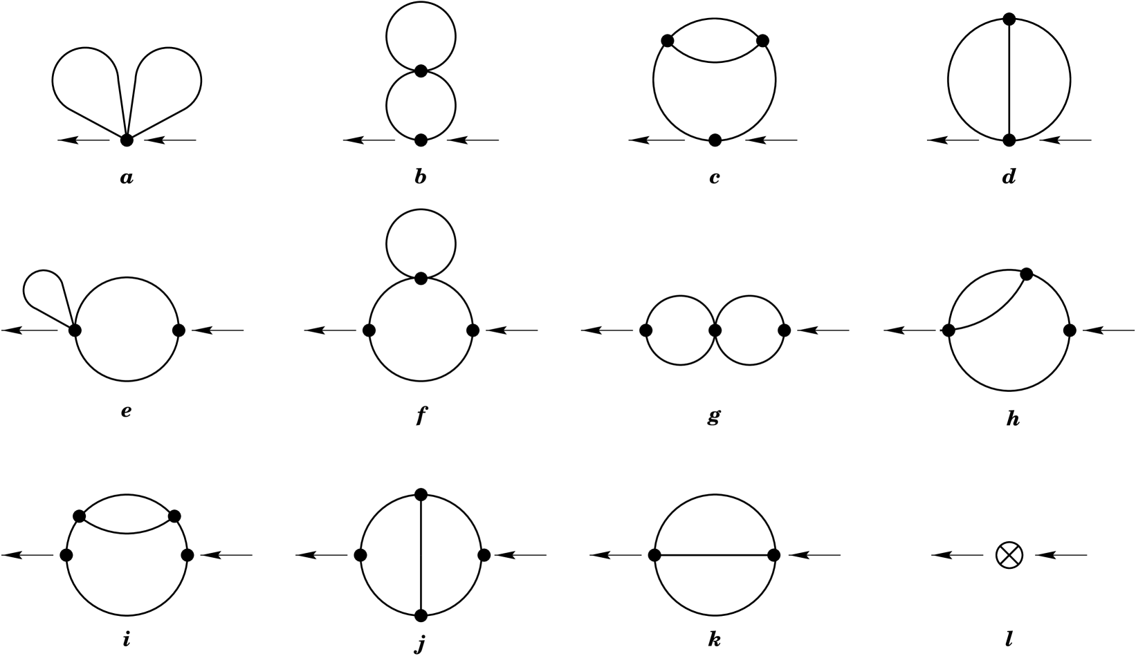
Figure 16: Two-loop diagrams contributing to the irreducible part $\tilde{C}_{ab}({\bf k})$ of the density-density correlator. The arrows merely serve to indicate where external momentum flows in and out of each diagram; the vertices where momentum flows in and out should be regarded as having attached species labels $a$ and $b$, respectively. The circled ‘X’ in diagram $l$ denotes the contribution from the two-loop interactions proportional to either $g^{0}_{ab}$ or $h^{0}_{a}$. Diagrams $a$–$d$ are two loop contributions to the contact term $\delta_{ab}\left\langle n_{a}\right\rangle_{\beta}$. These terms, together with part of diagram $l$, simply provide the two-loop correction to the number density $\left\langle n_{a}\right\rangle_{\beta}$. Not shown are reflected versions of diagrams $e$ and $h$ which differ only by an interchange of incoming and outgoing vertices. Diagram $e$ and its reflection are one-loop corrections to the densities that appear in the vertex factors in the one-loop result for $\tilde{C}_{ab}({\bf k})$. Diagram $f$ is a one-loop density correction to the Debye wave number in the Debye Green’s function appearing in the one-loop $\tilde{C}_{ab}({\bf k})$. Thus, the effect of diagrams $a$ through $f$ (plus a part of $l$) is merely to put the correct physical densities, to two-loop order, in the previous one-loop $\tilde{C}_{ab}({\bf k})$. Only diagrams $g$ through $k$ (plus the remaining part of $l$) give non-trivial, two-loop corrections to $\tilde{C}_{ab}({\bf k})$.

The two-loop diagrams contributing to the irreducible part $\tilde{C}_{ab}({\bf k})$ of the number density correlation function are shown in figure 16. Diagrams $a$–$d$ represent (momentum independent) contributions to the contact term $\delta_{ab}\left\langle n_{a}\right\rangle_{\beta}$. As noted earlier, only diagrams $d$ and $k$ (plus the induced coupling contribution $l$) are singular as $\nu\to 3$; all the other diagrams may be evaluated directly in three dimensions. The explicit contributions of these diagrams to $\tilde{C}_{ab}({\bf k})$ are given by

$$\Sigma_{a} = \delta_{ab}\,\beta^{2}\,n^{0}_{a}\,\,e_{a}^{4}\,\,{1\over 2^{3}}\,G_{3}({\bf 0})^{2}\,,$$ (4.22)

$$\Sigma_{b} = -\delta_{ab}\sum_{c}\beta^{3}\,n^{0}_{a}\,n^{0}_{c}\,\,e_{a}^{2}\,e_{c}^{4}\,\,{1\over 2^{2}}\,D^{(2)}_{3}({\bf 0})\,G_{3}({\bf 0})\,,$$ (4.23)

$$\Sigma_{c} = \delta_{ab}\sum_{c,d}\beta^{4}\,n^{0}_{a}\,n^{0}_{c}\,n^{0}_{d}\,\,e_{a}^{2}\,e_{c}^{3}\,e_{d}^{3}\,\,{1\over 2^{2}}\,D^{(121)}_{3}({\bf 0})\,,$$ (4.24)

$$\Sigma_{d} = -\delta_{ab}\sum_{c}\beta^{3}\,n^{0}_{a}\,n^{0}_{c}\,\,e_{a}^{3}\,e_{c}^{3}\,\,{1\over 3!}\,D^{(3)}_{\nu}({\bf 0})\,,$$ (4.25)

$$\Sigma_{e} = -\beta^{3}\,n^{0}_{a}\,n^{0}_{b}\,\left(e_{a}^{4}\,e_{b}^{2}+e_{a}^{2}\,e_{b}^{4}\right){1\over 2^{2}}\,D^{(2)}_{3}({\bf k})\,G_{3}({\bf 0})\,,$$ (4.26)

$$\Sigma_{f} = \sum_{c}\beta^{4}\,n^{0}_{a}\,n^{0}_{b}\,n^{0}_{c}\,\,e_{a}^{2}\,e_{b}^{2}\,e_{c}^{4}\,\,{1\over 2}\,D^{(111)}_{3}({\bf k})\,G_{3}({\bf 0})\,,$$ (4.27)

$$\Sigma_{g} = \sum_{c}\beta^{4}\,n^{0}_{a}\,n^{0}_{b}\,n^{0}_{c}\,\,e_{a}^{2}\,e_{b}^{2}\,e_{c}^{4}\,\,{1\over 2^{2}}\,D^{(2)}_{3}({\bf k})^{2}\,,$$ (4.28)

$$\Sigma_{h} = \sum_{c}\beta^{4}\,n^{0}_{a}\,n^{0}_{b}\,n^{0}_{c}\,\left(e_{a}^{3}\,e_{b}^{2}+e_{a}^{2}\,e_{b}^{3}\right)e_{c}^{3}\,\,{1\over 2}\,D^{(211)}_{3}({\bf k})\,,$$ (4.29)

$$\Sigma_{i} = -\sum_{c,d}\beta^{5}\,n^{0}_{a}\,n^{0}_{b}\,n^{0}_{c}\,n^{0}_{d}\,\,e_{a}^{2}\,e_{b}^{2}\,e_{c}^{3}\,e_{d}^{3}\,\,{1\over 2}D^{(1211)}_{3}({\bf k})\,,$$ (4.30)

$$\Sigma_{j} = -\sum_{c,d}\beta^{5}\,n^{0}_{a}\,n^{0}_{b}\,n^{0}_{c}\,n^{0}_{d}\,\,e_{a}^{2}\,e_{b}^{2}\,e_{c}^{3}\,e_{d}^{3}\,\,{1\over 2}D_{J}({\bf k})\,,$$ (4.31)

$$\Sigma_{k} = -\beta^{3}\,n^{0}_{a}\,n^{0}_{b}\,\,e_{a}^{3}\,e_{b}^{3}\,\,{1\over 3!}\,D^{(3)}_{\nu}({\bf k})\,,$$ (4.32)

$$\Sigma_{l} = -2\beta^{3}\,g^{0}_{ab}\,n^{0}_{a}\,n^{0}_{b}\,-2\delta_{ab}\sum_{c}\beta^{3}\,g^{0}_{ac}\,n^{0}_{a}\,n^{0}_{c}\vphantom{{1\over 1}}-2\,\delta_{ab}\,\beta^{2}\,h^{0}_{a}\,n^{0}_{a}\,{\bf k}^{2}\,,$$ (4.33)

where the required integrals are

$$D^{(n)}_{\nu}({\bf k}) \equiv \int(d^{\nu}{\bf r})\>e^{-i{\bf k}\cdot{\bf r}}\,G_{\nu}({\bf r})^{n}\,,$$ (4.34)

$$D^{(lmn)}_{\nu}({\bf k}) \equiv \int(d^{\nu}{\bf r})(d^{\nu}{\bf r}_{1})\>e^{-i{\bf k}\cdot{\bf r}}\,G_{\nu}({\bf r}{-}{\bf r}_{1})^{l}G_{\nu}({\bf r}_{1})^{m}G_{\nu}({\bf r})^{n}\,,$$ (4.35)

$$D^{(klmn)}_{\nu}({\bf k}) \equiv \int(d^{\nu}{\bf r})(d^{\nu}{\bf r}_{1})(d^{\nu}{\bf r}_{2})\>e^{-i{\bf k}\cdot{\bf r}}\,G_{\nu}({\bf r}{-}{\bf r}_{1})^{k}G_{\nu}({\bf r}_{1}{-}{\bf r}_{2})^{l}G_{\nu}({\bf r}_{2})^{m}G_{\nu}({\bf r})^{n}\,,$$ (4.36)

$$D_{J}({\bf k}) \equiv \int(d^{3}{\bf r})(d^{3}{\bf r}_{1})(d^{3}{\bf r}_{2})\>e^{-i{\bf k}\cdot{\bf r}}\,G_{3}({\bf r}{-}{\bf r}_{1})G_{3}({\bf r}{-}{\bf r}_{2})G_{3}({\bf r}_{1}{-}{\bf r}_{2})G_{3}({\bf r}_{1})G_{3}({\bf r}_{2})\,.$$ (4.37)

These integrals are evaluated in Appendix C.2 (with help from Ref. [32]).

By examining the graphical structure, it is easy to see that the irreducible density correlator has the form

$$\tilde{C}_{ab}({\bf k})=\delta_{ab}\,\bar{n}_{a}\,\tilde{F}_{a}({\bf k})+{\textstyle{1\over 2}}\left(\beta e_{a}^{2}\bar{n}_{a}\right)\tilde{F}_{ab}({\bf k})\left(\beta e_{b}^{2}\bar{n}_{b}\right)\,,$$ (4.38)

which generalizes the one-loop result (2.104). The derivative interaction involving the induced coupling $h^{0}_{a}$ is responsible for generating the ${\bf k}$-dependence in the $\delta_{ab}$ contact term,

$$\tilde{F}_{a}^{(2)}({\bf k})=1-2\beta^{2}\,h^{0}_{a}\,{\bf k}^{2}\,.$$ (4.39)

The terms $\Sigma_{a}$ through $\Sigma_{d}$, together with the second part of the renormalization term $\Sigma_{l}$, just give the two-loop corrections to the number density $\langle n_{a}\rangle_{\beta}$ that appears in $\delta_{ab}\,\bar{n}_{a}$ in the general form above. It is straightforward to show that these terms are just the two-loop parts in the previous result (4.10) for the number density. The one-loop correction, given in Eq. (2.104), involves

$$\tilde{F}_{ab}^{(1)}({\bf k})=D_{3}^{(2)}({\bf k})\,.$$ (4.40)

Recalling that the one-loop density correction reads

$$\delta\langle n_{a}\rangle_{\beta}=-{\textstyle{1\over 2}}\beta\,e_{a}^{2}\,G_{3}({\bf 0})\,n^{0}_{a}\,,$$ (4.41)

we see that the two-loop term $\Sigma_{e}$ gives the one-loop correction for each of the two explicit density factors appearing in the second term of (4.38), with $\tilde{F}_{ab}({\bf k})$ taking on its one-loop value $D_{3}^{(2)}({\bf k})$. Writing out $D^{(111)}_{3}({\bf k})$ in terms of Fourier integrals [as is done explicitly in Eq. (C.39)], it is easy to see that

$$D^{(111)}_{3}({\bf k})=-{1\over 2}{dD^{(2)}_{3}({\bf k})\over d\kappa_{0}^{2}}\,.$$ (4.42)

Therefore $\Sigma_{f}$ accounts for the correction to the one-loop $\tilde{F}_{ab}^{(1)}({\bf k})$ brought about by replacing the bare Debye wave number $\kappa_{0}$ by its one-loop corrected value. In summary, the two-loop terms $\Sigma_{a}$ through $\Sigma_{f}$, plus the second piece of $\Sigma_{l}$, just provide simple density corrections to the one-loop $\tilde{C}_{ab}^{(1)}({\bf k})$, and all of these terms may be omitted if the correct physical densities $\bar{n}_{a}$ are used in the construction of $\tilde{C}_{ab}^{(1)}({\bf k})$.

To assemble the remaining terms in the two-loop, irreducible correlator, we first use the explicit form (3.41) of the induced coupling $g^{0}_{ab}$ to write the sum of $\Sigma_{k}$ and the first piece of $\Sigma_{l}$ as

$$\Sigma_{k}({\bf k})-2\beta^{3}\,g^{0}_{ab}\,n^{0}_{a}\,n^{0}_{b}=-\beta^{3}\,n^{0}_{a}\,n^{0}_{b}\left[{1\over 3!}\,\left(e_{a}^{3}e_{b}^{3}\right)D^{(3)}_{\rm R}({\bf k};\mu)+2g_{ab}(\mu)\right]$$ (4.43)

where

$$D^{(3)}_{\rm R}({\bf k};\mu)\equiv D^{(3)}_{\nu}({\bf k})-{1\over 2(4\pi)^{2}}\,{\mu^{2(\nu-3)}\over 3-\nu}\,.$$ (4.44)

This is the generalization to non-vanishing wave number of $D_{\rm R}^{(3)}({\bf 0};\mu)$ previously introduced in Eq. (4.5). Using the result (C.30) for $D_{\nu}^{(3)}({\bf k})$ in dispersion relation form and taking the physical $\nu\to 3$ limit yields

$$D_{\rm R}^{(3)}({\bf k};\mu)=-{1\over(4\pi)^{2}}\,{1\over 2}\Bigg{\{}\ln\left({9\kappa^{2}\over 4\pi\mu^{2}}\right)-3+\gamma+2\int_{3\kappa}^{\infty}ds\left({k^{2}\over s}+3\kappa\right){1\over k^{2}+s^{2}}\Bigg{\}}\,.$$ (4.45)

Alternatively, using the result (C.31) for $D_{\nu}^{(3)}({\bf k})$ evaluated in terms of elementary functions gives the $\nu=3$ limit

$$D^{(3)}_{\rm R}({\bf k};\mu)=-{1\over(4\pi)^{2}}\,{1\over 2}\left\{\ln\left({9\kappa^{2}\over 4\pi\mu^{2}}\right)-3+\gamma+{6\kappa\over k}\arctan{k\over 3\kappa}+\ln\biggl{[}1+{k^{2}\over 9\kappa^{2}}\biggr{]}\right\}.$$ (4.46)

Combining the one-loop result (4.40) with this renormalized contribution of $\Sigma_{k}$ plus the other non-trivial two-loop terms $\Sigma_{g}$ through $\Sigma_{j}$, and recalling the definition (6.3) of the coupling $g_{ab}(\mu)$, leads to

$$\tilde{F}_{ab}^{(2)}({\bf k}) = D_{3}^{(2)}({\bf k})\Bigl{[}1+{\textstyle{1\over 2}}\sum_{c}\beta^{2}\,\bar{n}_{c}\,e^{4}_{c}\,D_{3}^{(2)}({\bf k})\Bigr{]}+\sum_{c}\beta^{2}\,\bar{n}_{c}\,\left(e_{a}+e_{b}\right)\,e_{c}^{3}\,D_{3}^{(211)}({\bf k})$$ (4.47)

$$\quad-\sum_{c,d}\beta^{3}\,\bar{n}_{c}\,\bar{n}_{d}\,e^{3}_{c}\,e^{3}_{d}\,\left[D_{3}^{(1211)}({\bf k})+D_{J}({\bf k})\right]$$

$$\quad-{\textstyle{1\over 3}}\,\beta\,e_{a}\,e_{b}\left[D_{\rm R}^{(3)}({\bf k})-{\textstyle{1\over 2}}\,(4\pi)^{-2}\left(\ln\mu^{2}\lambda_{ab}^{2}+\Gamma_{ab}\right)\right].$$

The functions $D_{3}^{(2)}({\bf k})$, $D_{3}^{(211)}({\bf k})$, and $D_{3}^{(1211)}({\bf k})$ are given in dispersion relation form in Eq’s. (C.21), (C.51), and (C.52) of Appendix C. The same functions are also expressed in terms of elementary functions and the Euler dilogarithm (or Spence function) in Eq’s. (C.21), (C.56), and (C.57). The function $D_{J}({\bf k})$ is not so tractable. However, it has been expressed in terms of a one-dimensional integral by Rajantie [32]. His result is quoted in Eq. (C.73) of Appendix C.

The ${\bf k}\to 0$ limit of the irreducible correlator is related to the particle number fluctuations. Using the results (C.22), (C.53), (C.54), and (C.74) for $D_{3}^{(2)}({\bf 0})$, $D_{3}^{(211)}({\bf 0})$, $D_{3}^{(1211)}({\bf 0})$ and $D_{J}({\bf 0})$, plus Eq. (4.6) for $D_{\rm R}^{(3)}({\bf 0})$, we have

$$\tilde{F}^{(2)}_{ab}({\bf 0}) = {1\over 8\pi\kappa}\left[1+{1\over 2}\sum_{c}{\beta^{2}\,\bar{n}_{c}\,e_{c}^{4}\over 8\pi\kappa}\right]+{1\over 6}\sum_{c}\bar{n}_{c}\,{\beta^{2}\,\left(e_{a}{+}e_{b}\right)e_{c}^{3}\over(4\pi)^{2}\,\kappa^{2}}$$ (4.48)

$$\qquad{}-{1\over 12}\sum_{c,d}\bar{n}_{c}\,\bar{n}_{d}\,{\beta^{3}e_{c}^{3}e_{d}^{3}\over(4\pi)^{2}\,\kappa^{4}}+{1\over 6}\,{\beta e_{a}e_{b}\over(4\pi)^{2}}\left[\ln\!\left({9\lambda_{ab}^{2}\kappa^{2}\over 4\pi}\right)-1+\gamma+\Gamma_{ab}\right].$$

To check this result, we note that, as is shown in Eq. (A.68) of Appendix A, there is a simpler way to obtain the same result, namely:

$$\tilde{C}_{ab}({\bf 0})=-{\partial\langle n_{a}\rangle_{\beta}\over\partial\beta\mu_{b}}=-{\partial\langle n_{b}\rangle_{\beta}\over\partial\beta\mu_{a}}\,,$$ (4.49)

where the partial derivatives are to be computed at fixed $\beta$. It is a straight forward matter to take the $\beta\mu_{b}$ derivative of the two-loop result (4.10) for the density $\langle n_{a}\rangle_{\beta}$ and confirm [via Eq. (4.38)] that the result (4.48) is indeed correct.

5 Three-Loop Thermodynamics

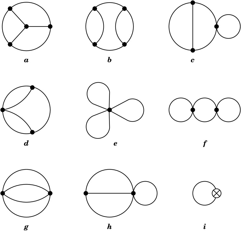
Figure 17: Three-loop diagrams contributing to the $\ln Z$. The circled ‘X’ denotes the insertion of the part of the two-loop $g^{0}_{ab}$ and $h^{0}_{a}$ interactions which are quadratic in $\phi$.

There are nine diagrams, shown in figure 17, which contribute to $\ln Z$ (or equivalently the pressure) at three-loop order. Diagrams $a$–$f$ are finite as $\nu\to 3$ and may be computed directly in 3 dimensions. The explicit contributions of these diagrams to $(\ln Z)/{\cal V}$ are:

$$\Gamma_{a}+\Gamma_{b} = \sum_{a,b,c,d}\beta^{6}\,n^{0}_{a}\,n^{0}_{b}\,n^{0}_{c}\,n^{0}_{d}\,\,e_{a}^{3}\,e_{b}^{3}\,e_{c}^{3}\,e_{d}^{3}\,\,\left[{1\over 4!}\,D_{M}+{1\over 2^{4}}\,D^{(2121)}_{3}({\bf 0})\right],$$ (5.1)

$$\Gamma_{c}+\Gamma_{d} = -\sum_{a,b,c}\beta^{5}\,n^{0}_{a}\,n^{0}_{b}\,n^{0}_{c}\,\,e_{a}^{4}\,e_{b}^{3}\,e_{c}^{3}\,\,\left[{1\over 2^{3}}\,D^{(211)}_{3}({\bf 0})\,G_{3}({\bf 0})+{1\over 2^{3}}\,D^{(221)}_{3}({\bf 0})\right],$$ (5.2)

$$\Gamma_{e} = -\sum_{a}\beta^{3}\,n^{0}_{a}\,\,e_{a}^{6}\,\,{1\over 2^{3}\cdot 3!}\,G_{3}({\bf 0})^{3}$$ (5.3)

$$\Gamma_{f}+\Gamma_{g} = \sum_{a,b}\beta^{4}\,n^{0}_{a}\,n^{0}_{b}\,\,e_{a}^{4}\,e_{b}^{4}\,\left[{1\over 2^{4}}\,D^{(2)}_{3}({\bf 0})\,G_{3}({\bf 0})^{2}+{1\over 2\cdot 4!}\,D^{(4)}_{\nu}({\bf 0})\right],$$ (5.4)

$$\Gamma_{h} = \sum_{a,b}\beta^{4}\,n^{0}_{a}\,n^{0}_{b}\,\,e_{a}^{5}\,e_{b}^{3}\,\,{1\over 2\cdot 3!}\,D^{(3)}_{\nu}({\bf 0})\,G_{\nu}({\bf 0})\,,$$ (5.5)

$$\Gamma_{i} = \sum_{a,b}\beta^{4}\,g^{0}_{ab}\,n^{0}_{a}\,n^{0}_{b}\left(e_{a}{+}e_{b}\right)^{2}\,{1\over 2}\,G_{\nu}({\bf 0})-\sum_{a}\beta^{4}\,h^{0}_{a}\,n^{0}_{a}\,e_{a}^{2}\,\kappa_{0}^{2}\,G_{\nu}({\bf 0})\,.$$ (5.6)

The last term of Eq. (5.6) comes from

$$\beta\left<\!\left<\nabla\phi({\bf r})^{2}\right>\!\right>^{(0)}=-\kappa_{0}^{2}\,G_{\nu}({\bf 0})\mathop{\longrightarrow}_{\nu\to 3}{\kappa_{0}^{3}\over 4\pi}\,,$$ (5.7)

which easily follows using the same method that lead to Eq. (2.60). The integral

$$D_{M} \equiv \int(d^{3}{\bf r})(d^{3}{\bf r}^{\prime})(d^{3}{\bf r}^{\prime\prime})\>G_{3}({\bf r})\,G_{3}({\bf r}^{\prime})\,G_{3}({\bf r}^{\prime\prime})\,G_{3}({\bf r}{-}{\bf r}^{\prime})\,G_{3}({\bf r}^{\prime}{-}{\bf r}^{\prime\prime})\,G_{3}({\bf r}^{\prime\prime}{-}{\bf r})$$ (5.8)

corresponds to the “Mercedes” graph $a$ of Fig. 17, and the other required integrals are defined in Eq’s. (4.34)–(4.36). These integrals are evaluated in Appendix C.2 (with help from Refs. [32, 33]). Once again, the final contribution $\Gamma_{i}$ involving the single two-loop coupling $g^{0}_{ab}$ removes the short-distance singularities in both the three-loop graphs $\Gamma_{g}$ and $\Gamma_{h}$ that diverge in three dimensions. Note that this cancelation of divergences involves the detailed structure of the induced coupling interaction with its exponential dependence upon the potential $\phi$. As discussed earlier, the basic (“primitive”) divergences which the induced couplings must cancel appear only in even loop order. The subsidiary divergences at this three-loop order are canceled by the non-trivial potential dependence of the two-loop induced coupling. Inserting the explicit results for these integrals produces the physical $\nu\to 3$ limit of $\ln Z$ to three loop order:

$${\ln Z_{3}\over{\cal V}}={\ln Z_{2}\over{\cal V}} + {1\over 4!\,(4\pi)^{3}}\,\Biggl{\{}\,\sum_{a,b,c,d}\beta^{6}\,n^{0}_{a}\,n^{0}_{b}\,n^{0}_{c}\,n^{0}_{d}\,\,e_{a}^{3}\,e_{b}^{3}\,e_{c}^{3}\,e_{d}^{3}\,\,{C_{1}\over\kappa_{0}^{3}}$$ (5.9)

$$\quad\qquad{}+\sum_{a,b,c}\beta^{5}\,n^{0}_{a}\,n^{0}_{b}\,n^{0}_{c}\,\,e_{a}^{4}\,e_{b}^{3}\,e_{c}^{3}\,\,{C_{2}\over\kappa_{0}}$$

$$\quad\qquad{}+\sum_{a}\beta^{3}\,n^{0}_{a}\,\,e_{a}^{6}\,\,\kappa_{0}^{3}\,\left[C_{3}+{8\pi\lambda_{a}^{2}\over\beta^{2}\,e_{a}^{4}}\right]$$

$$\quad\qquad{}+\sum_{a,b}\beta^{4}\,n^{0}_{a}\,n^{0}_{b}\,\,e_{a}^{4}\,e_{b}^{4}\,\,\kappa_{0}\left[C_{4}+\ln\!\left({9\lambda_{ab}^{2}\bar{\kappa}^{2}\over 4\pi}\right)+\Gamma_{ab}\right]$$

$$\quad\qquad{}+\sum_{a,b}\beta^{4}\,n^{0}_{a}\,n^{0}_{b}\,\,e_{a}^{5}\,e_{b}^{3}\,\,\kappa_{0}\left[C_{5}+\ln\!\left({9\lambda_{ab}^{2}\bar{\kappa}^{2}\over 4\pi}\right)+\Gamma_{ab}\right]\Biggr{\}},$$

with

$$C_{1} = C_{M}+{\textstyle{3\over 4}}\,{\rm Li}_{2}(-{\textstyle{1\over 3}})+\ln{\textstyle{3\over 4}}+{\textstyle{\pi^{2}\over 16}}=0.119131\cdots\,,$$ (5.10)

$$C_{2} = -3\,{\rm Li}_{2}(-{\textstyle{1\over 3}})+{\textstyle{1\over 2}}-{\textstyle{\pi^{2}\over 4}}=-1.04030\cdots\,,$$ (5.11)

$$C_{3} = {\textstyle{1\over 2}}\,,$$ (5.12)

$$C_{4} = \gamma-{\textstyle{9\over 4}}-2\ln{\textstyle{3\over 4}}=-1.09742\cdots\,,$$ (5.13)

$$C_{5} = \gamma-1=-0.422784\cdots\,,$$ (5.14)

where

$${\rm Li}_{2}(-z)\equiv-\int_{0}^{z}{dt\over t}\>\ln(1+t)\,.$$ (5.15)

is Euler’s dilogarithm, $C_{M}$ is given in Eq. (C.70), and $\Gamma_{ab}$ was defined in Eq. (3.82).

Differentiating Eq. (5.9) with respect to $\beta$ yields the internal energy, in terms of bare parameters, to three loop order:

$$\beta u = \sum_{a=1}^{A}n^{0}_{a}\>\Biggl{\{}{3\over 2}+{1\over 4}\left({\beta e_{a}^{2}\kappa_{0}\over 4\pi}\right)-{C_{3}\over 32}\left({\beta e_{a}^{2}\kappa_{0}\over 4\pi}\right)^{3}+{1\over 48}\left({\kappa_{0}^{2}\lambda_{a}^{2}\over 4\pi}\right)\left({\beta e_{a}^{2}\kappa_{0}\over 4\pi}\right)\Biggr{\}}$$ (5.16)

$$- \sum_{a,b=1}^{A}n^{0}_{a}\,n^{0}_{b}\left\{{1\over 48}\left({\beta^{3}e_{a}^{3}e_{b}^{3}\over(4\pi)^{2}}\right)\left[1+\eta_{ab}\Gamma^{\prime}_{ab}\right]\right.$$

$$\kern 50.58878pt\left.{}+{1\over 32}\left({\beta^{4}e_{a}^{5}e_{b}^{3}\kappa_{0}\over(4\pi)^{3}}\right)\left[C_{5}+{\textstyle{2\over 3}}+\ln\!\left({9\lambda_{ab}^{2}\bar{\kappa}^{2}\over 4\pi}\right)+\Gamma_{ab}+{\textstyle{2\over 3}}\eta_{ab}\Gamma^{\prime}_{ab}\right]\right.$$

$$\kern 50.58878pt\left.{}+{1\over 32}\left({\beta^{4}e_{a}^{4}e_{b}^{4}\kappa_{0}\over(4\pi)^{3}}\right)\left[C_{4}+{\textstyle{2\over 3}}+\ln\!\left({9\lambda_{ab}^{2}\bar{\kappa}^{2}\over 4\pi}\right)+\Gamma_{ab}+{\textstyle{2\over 3}}\eta_{ab}\Gamma^{\prime}_{ab}\right]\right\}$$

$$- \sum_{a,b,c=1}^{A}n^{0}_{a}\,n^{0}_{b}\,n^{0}_{c}\left\{{C_{2}\over 32}\left({\beta^{5}e_{a}^{4}e_{b}^{3}e_{c}^{3}\over\kappa_{0}\,(4\pi)^{3}}\right)\right\}$$

$$- \sum_{a,b,c,d=1}^{A}n^{0}_{a}\,n^{0}_{b}\,n^{0}_{c}\,n^{0}_{d}\left\{{C_{1}\over 32}\left({\beta^{6}e_{a}^{3}e_{b}^{3}e_{c}^{3}e_{d}^{3}\over\kappa_{0}^{3}\,(4\pi)^{3}}\right)\right\},$$

while differentiating with respect to the chemical potentials yields the particle densities (in terms of bare parameters) to three loop order:

$$\bar{n}_{s}=\left\langle n_{s}\right\rangle_{\beta} = n^{0}_{s}\left[1+\left({\beta e_{s}^{2}\kappa_{0}\over 8\pi}\right)+{1\over 2}\left({\beta e_{s}^{2}\kappa_{0}\over 8\pi}\right)^{2}+{2C_{3}\over 3!}\left({\beta e_{s}^{2}\kappa_{0}\over 8\pi}\right)^{3}+{1\over 12}\left({\beta e_{s}^{2}\kappa_{0}\over 4\pi}\right)\left({\kappa_{0}^{2}\lambda_{s}^{2}\over 4\pi}\right)\right.$$ (5.17)

$${}+\sum_{a=1}^{A}n^{0}_{a}\left\{{1\over 8}\left({\beta^{3}e_{s}^{2}e_{a}^{4}\over(4\pi)^{2}}\right)+{1\over 12}\left({\beta^{3}e_{s}^{3}e_{a}^{3}\over(4\pi)^{2}}\right)\left[\gamma-1+\ln\!\left({\textstyle{9\over 4}}\lambda_{as}^{2}\kappa_{0}^{2}/\pi\right)+\Gamma_{as}\right]\right.$$

$$\kern 108.405pt{}+{C_{3}\over 16}\left({\beta^{4}e_{s}^{2}e_{a}^{6}\kappa_{0}\over(4\pi)^{3}}\right)+{\kappa_{0}\over 8}\left({\beta^{2}e_{s}^{2}e_{a}^{2}\lambda_{a}^{2}\over(4\pi)^{2}}\right)$$

$$\kern 108.405pt{}+{\kappa_{0}\over 12}\left({\beta^{4}e_{s}^{4}e_{a}^{4}\over(4\pi)^{3}}\right)\left[C_{4}+\ln\!\left({\textstyle{9\over 4}}\lambda_{as}^{2}\bar{\kappa}^{2}/\pi\right)+\Gamma_{as}\right]$$

$$\kern 108.405pt\left.{}+{\kappa_{0}\over 24}\left({\beta^{4}[e_{s}^{3}e_{a}^{5}{+}e_{s}^{5}e_{a}^{3}]\over(4\pi)^{3}}\right)\left[C_{5}+\ln\!\left({\textstyle{9\over 4}}\lambda_{as}^{2}\bar{\kappa}^{2}/\pi\right)+\Gamma_{as}\right]\right\}$$

$${}+\sum_{a,b=1}^{A}n^{0}_{a}n^{0}_{b}\left\{{1\over 24}\left({\beta^{4}e_{s}^{2}e_{a}^{3}e_{b}^{3}\over\kappa_{0}^{2}\,(4\pi)^{2}}\right)+{C_{2}\over 24}\left({\beta^{5}e_{s}^{4}e_{a}^{3}e_{b}^{3}\over\kappa_{0}\,(4\pi)^{3}}\right)+{C_{2}\over 12}\left({\beta^{5}e_{s}^{3}e_{a}^{4}e_{b}^{3}\over\kappa_{0}\,(4\pi)^{3}}\right)\right.$$

$$\kern 108.405pt{}+{1\over 48}\left({\beta^{5}e_{s}^{2}e_{a}^{5}e_{b}^{3}\over\kappa_{0}\,(4\pi)^{3}}\right)\left[C_{5}+2+\ln\!\left({\textstyle{9\over 4}}\lambda_{ab}^{2}\bar{\kappa}^{2}/\pi\right)+\Gamma_{ab}\right]$$

$$\kern 108.405pt\left.{}+{1\over 48}\left({\beta^{5}e_{s}^{2}e_{a}^{4}e_{b}^{4}\over\kappa_{0}\,(4\pi)^{3}}\right)\left[C_{4}+2+\ln\!\left({\textstyle{9\over 4}}\lambda_{ab}^{2}\bar{\kappa}^{2}/\pi\right)+\Gamma_{ab}\right]\right\}$$

$${}-\sum_{a,b,c=1}^{A}n^{0}_{a}\,n^{0}_{b}\,n^{0}_{c}\left\{{C_{2}\over 48}\left({\beta^{6}e_{s}^{2}e_{a}^{4}e_{b}^{3}e_{c}^{3}\over\kappa_{0}^{3}\,(4\pi)^{3}}\right)-{C_{1}\over 6}\left({\beta^{6}e_{s}^{3}e_{a}^{3}e_{b}^{3}e_{c}^{3}\over\kappa_{0}^{3}\,(4\pi)^{3}}\right)\right\}$$

$$\left.{}-\sum_{a,b,c,d=1}^{A}n^{0}_{a}\,n^{0}_{b}\,n^{0}_{c}\,n^{0}_{d}\left\{{C_{1}\over 16}\left({\beta^{7}e_{s}^{2}e_{a}^{3}e_{b}^{3}e_{c}^{3}e_{d}^{3}\over\kappa_{0}^{5}\,(4\pi)^{3}}\right)\right\}\right].$$

Inverting the relation between physical and bare densities, and inserting the explicit values for $C_{3}$, $C_{4}$ and $C_{5}$ (because this simplifies the subsequent results), yields

$$n^{0}_{s} = \bar{n}_{s}\left[1-\left({\beta e_{s}^{2}\bar{\kappa}\over 8\pi}\right)+{1\over 2}\left({\beta e_{s}^{2}\bar{\kappa}\over 8\pi}\right)^{2}-{1\over 3!}\left({\beta e_{s}^{2}\bar{\kappa}\over 8\pi}\right)^{3}-{1\over 6}\left({\beta e_{s}^{2}\bar{\kappa}\over 8\pi}\right)\left({\bar{\kappa}^{2}\lambda_{s}^{2}\over 4\pi}\right)\right.$$ (5.18)

$${}-\sum_{a=1}^{A}\bar{n}_{a}\left\{{1\over 12}\left({\beta^{3}e_{s}^{3}e_{a}^{3}\over(4\pi)^{2}}\right)\left[\gamma-1+\ln({{\textstyle{9\over 4}}\lambda_{as}^{2}\bar{\kappa}^{2}/\pi})+\Gamma_{as}\right]\right.$$

$$\;\quad\qquad\left.{}+{\bar{\kappa}\over 12}\left({\beta^{4}e_{s}^{4}e_{a}^{4}\over(4\pi)^{3}}\right)\left[\gamma-3+\ln\!\left(4\lambda_{as}^{2}\bar{\kappa}^{2}/\pi\right)+\Gamma_{as}\right]\right.$$

$$\;\quad\qquad\left.{}-{\bar{\kappa}\over 24}\left({\beta^{4}e_{s}^{5}e_{a}^{3}\over(4\pi)^{3}}\right)\left[\gamma-1+\ln\!\left({\textstyle{9\over 4}}\lambda_{as}^{2}\bar{\kappa}^{2}/\pi\right)+\Gamma_{as}\right]+{\bar{\kappa}\over 8}\left({\beta^{2}e_{s}^{2}e_{a}^{2}\lambda_{a}^{2}\over(4\pi)^{2}}\right)\right\}$$

$${}-\sum_{a,b=1}^{A}\bar{n}_{a}\bar{n}_{b}\left\{{1\over 24}\left({\beta^{4}e_{s}^{2}e_{a}^{3}e_{b}^{3}\over\bar{\kappa}^{2}\,(4\pi)^{2}}\right)+{C_{2}{-}1\over 24}\left({\beta^{5}e_{s}^{4}e_{a}^{3}e_{b}^{3}\over\bar{\kappa}\,(4\pi)^{3}}\right)+{C_{2}{-}{\textstyle{1\over 2}}\over 12}\left({\beta^{5}e_{s}^{3}e_{a}^{4}e_{b}^{3}\over\bar{\kappa}\,(4\pi)^{3}}\right)\right.$$

$$\;\;\qquad\qquad\left.{}+{1\over 48}\left({\beta^{5}e_{s}^{2}e_{a}^{4}e_{b}^{4}\over\bar{\kappa}\,(4\pi)^{3}}\right)\left[\gamma-1+\ln\!\left(4\lambda_{ab}^{2}\bar{\kappa}^{2}/\pi\right)+\Gamma_{ab}\right]\right\}$$

$${}+\sum_{a,b,c=1}^{A}\bar{n}_{a}\,\bar{n}_{b}\,\bar{n}_{c}\left\{{C_{2}{-}{\textstyle{1\over 2}}\over 48}\left({\beta^{6}e_{s}^{2}e_{a}^{4}e_{b}^{3}e_{c}^{3}\over\bar{\kappa}^{3}\,(4\pi)^{3}}\right)-{C_{1}\over 6}\left({\beta^{6}e_{s}^{3}e_{a}^{3}e_{b}^{3}e_{c}^{3}\over\bar{\kappa}^{3}\,(4\pi)^{3}}\right)\right\}$$

$$\left.{}+\sum_{a,b,c,d=1}^{A}\bar{n}_{a}\,\bar{n}_{b}\,\bar{n}_{c}\,\bar{n}_{d}\left\{{C_{1}\over 16}\left({\beta^{7}e_{s}^{2}e_{a}^{3}e_{b}^{3}e_{c}^{3}e_{d}^{3}\over\bar{\kappa}^{5}\,(4\pi)^{3}}\right)\right\}\right].$$

Using this result to express the pressure in terms of physical densities gives the equation of state

$$\beta p={\ln Z\over{\cal V}} = \sum_{a=1}^{A}\bar{n}_{a}\left\{1-{1\over 6}\left({\beta e_{a}^{2}\bar{\kappa}\over 4\pi}\right)-{1\over 8}\left({\beta e_{a}^{2}\bar{\kappa}\over 4\pi}\right)\left({\bar{\kappa}^{2}\lambda_{a}^{2}\over 4\pi}\right)\right\}$$ (5.19)

$$- \sum_{a,b=1}^{A}\bar{n}_{a}\,\bar{n}_{b}\left\{{1\over 24}\left({\beta^{3}e_{a}^{3}e_{b}^{3}\over(4\pi)^{2}}\right)\left[\gamma+\ln\!\left({\textstyle{9\over 4}}\lambda_{ab}^{2}\bar{\kappa}^{2}/\pi\right)+\Gamma_{ab}\right]\right.$$

$$\;\;\quad\qquad\left.{}+{1\over 16}\left({\beta^{4}e_{a}^{4}e_{b}^{4}\bar{\kappa}\over(4\pi)^{3}}\right)\left[\gamma-{\textstyle{7\over 3}}+\ln\!\left(4\lambda_{ab}^{2}\bar{\kappa}^{2}/\pi\right)+\Gamma_{ab}\right]\right\}$$

$$- \sum_{a,b,c=1}^{A}\bar{n}_{a}\,\bar{n}_{b}\,\bar{n}_{c}\left\{{1\over 16}\left({\beta^{5}e_{a}^{4}e_{b}^{3}e_{c}^{3}\over\bar{\kappa}\,(4\pi)^{3}}\right)\left[C_{2}-{\textstyle{1\over 2}}\right]\right\}$$

$$- \sum_{a,b,c,d=1}^{A}\bar{n}_{a}\,\bar{n}_{b}\,\bar{n}_{c}\,\bar{n}_{d}\left\{{1\over 16}\left({\beta^{6}e_{a}^{3}e_{b}^{3}e_{c}^{3}e_{d}^{3}\over\bar{\kappa}^{3}\,(4\pi)^{3}}\right)\left[\,C_{1}\right]\right\}.$$

The internal energy expressed in terms of the physical densities is given by

$$\beta u = \sum_{a=1}^{A}\bar{n}_{a}\left\{{3\over 2}-{1\over 2}\left({\beta e_{a}^{2}\bar{\kappa}\over 4\pi}\right)-{7\over 24}\left({\beta e_{a}^{2}\bar{\kappa}\over 4\pi}\right)\left({\bar{\kappa}^{2}\lambda_{a}^{2}\over 4\pi}\right)\right\}$$ (5.20)

$$- \sum_{a,b=1}^{A}\bar{n}_{a}\,\bar{n}_{b}\left\{{1\over 8}\left({\beta^{3}e_{a}^{3}e_{b}^{3}\over(4\pi)^{2}}\right)\left[\gamma-{\textstyle{1\over 3}}+\ln({\textstyle{9\over 4}}\lambda_{ab}^{2}\bar{\kappa}^{2}/\pi)+\Gamma_{ab}+{\textstyle{1\over 6}}\eta_{ab}\Gamma^{\prime}_{ab}\right]\right.$$

$$\;\quad\qquad\left.{}+{3\over 16}\left({\beta^{4}e_{a}^{4}e_{b}^{4}\,\bar{\kappa}\over(4\pi)^{3}}\right)\left[\gamma-{\textstyle{23\over 9}}+\ln\!\left(4\lambda_{ab}^{2}\bar{\kappa}^{2}/\pi\right)+\Gamma_{ab}+{\textstyle{1\over 9}}\eta_{ab}\Gamma^{\prime}_{ab}\right]\right\}$$

$$- \sum_{a,b,c=1}^{A}\bar{n}_{a}\,\bar{n}_{b}\,\bar{n}_{c}\left\{{3\over 16}\left({\beta^{5}e_{a}^{4}e_{b}^{3}e_{c}^{3}\over\bar{\kappa}\,(4\pi)^{3}}\right)\left[C_{2}-{\textstyle{1\over 2}}\right]\right\}$$

$$- \sum_{a,b,c,d=1}^{A}\bar{n}_{a}\,\bar{n}_{b}\,\bar{n}_{c}\,\bar{n}_{d}\left\{{3\over 16}\left({\beta^{6}e_{a}^{3}e_{b}^{3}e_{c}^{3}e_{d}^{3}\over\bar{\kappa}^{3}\,(4\pi)^{3}}\right)\left[\,C_{1}\right]\right\},$$

while the Helmholtz free energy is

$$\beta f = \sum_{a=1}^{A}\bar{n}_{a}\left\{-1+\ln(\bar{n}_{a}\lambda_{a}^{3}/g_{a})-{1\over 3}\left({\beta e_{a}^{2}\bar{\kappa}\over 4\pi}\right)-{1\over 12}\left({\beta e_{a}^{2}\bar{\kappa}\over 4\pi}\right)\left({\bar{\kappa}^{2}\lambda_{a}^{2}\over 4\pi}\right)\right\}$$ (5.21)

$$- \sum_{a,b=1}^{A}\bar{n}_{a}\,\bar{n}_{b}\left\{{1\over 24}\left({\beta^{3}e_{a}^{3}e_{b}^{3}\over(4\pi)^{2}}\right)\left[\gamma-1+\ln({\textstyle{9\over 4}}\lambda_{ab}^{2}\bar{\kappa}^{2}/\pi)+\Gamma_{ab}\right]\right.$$

$$\;\;\quad\qquad\left.{}+{1\over 24}\left({\beta^{4}e_{a}^{4}e_{b}^{4}\,\bar{\kappa}\over(4\pi)^{3}}\right)\left[\gamma-3+\ln\!\left(4\lambda_{ab}^{2}\bar{\kappa}^{2}/\pi\right)+\Gamma_{ab}\right]\right\}$$

$$- \sum_{a,b,c=1}^{A}\bar{n}_{a}\,\bar{n}_{b}\,\bar{n}_{c}\left\{{1\over 24}\left({\beta^{5}e_{a}^{4}e_{b}^{3}e_{c}^{3}\over\bar{\kappa}\,(4\pi)^{3}}\right)\left[C_{2}-{\textstyle{1\over 2}}\right]\right\}$$

$$- \sum_{a,b,c,d=1}^{A}\bar{n}_{a}\,\bar{n}_{b}\,\bar{n}_{c}\,\bar{n}_{d}\left\{{1\over 24}\left({\beta^{6}e_{a}^{3}e_{b}^{3}e_{c}^{3}e_{d}^{3}\over\bar{\kappa}^{3}\,(4\pi)^{3}}\right)\left[\,C_{1}\right]\right\}.$$

This result agrees with the corresponding result in Alastuey and Perez [7]. It also agrees, except for some small misprints and the omission of one quantum-mechanical term, with the result to be found in Ref. [6]. Note that the pressure is related to the Helmholtz free energy by the thermodynamic identity $p=-\left.\partial F/\partial{\cal V}\right|_{T,N}$. It is easy to apply this identity and verify that Eq. (5.19) follows from (5.21).

As explained in the next section, the combination

$$A=\beta(3p-u)-{\textstyle{3\over 2}}\sum_{a=1}^{A}\bar{n}_{a}$$ (5.22)

would vanish identically if the plasma could be treated entirely in a classical manner. However, the results above give

$$A=-{1\over(4\pi)^{2}}\left\{{1\over 24}\sum_{a,b=1}^{A}\bar{n}_{a}\,\bar{n}_{b}\,\beta^{3}e_{a}^{3}e_{b}^{3}\left[1-{\textstyle{1\over 2}}\,\eta_{ab}\,\Gamma^{\prime}_{ab}\right]\left[1+{\beta\,e_{a}e_{b}\,\bar{\kappa}\over 4\pi}\right]+{1\over 12}\sum_{a=1}^{A}\bar{n}_{a}\,\beta\,e_{a}^{2}\,\bar{\kappa}^{3}\,\lambda_{a}^{2}\right\}.$$

(5.23)

The next section shows how $A$ may be independently computed from quantum corrections to the virial theorem for a classical Coulomb plasma, and discusses how $A$ plays a role analogous to the anomalies which appear in relativistic quantum field theory.

5.1 Binary Plasma

These expressions simplify considerably for a two-component plasma such as an electron-proton plasma where $-e_{e}=e_{p}\equiv e$, and charge neutrality requires that $\bar{n}_{e}=\bar{n}_{p}\equiv n/2$. For example, the three-loop equation of state becomes

$${\beta\,p\over n}=1 - {1\over 3}\left({\beta e^{2}\bar{\kappa}\over 8\,\pi}\right)\left\{1+{3\over 8}\,{\bar{\kappa}^{2}(\lambda_{e}^{2}{+}\lambda_{p}^{2})\over 4\pi}\right\}$$ (5.24)

$$- {1\over 24}\left({\beta e^{2}\bar{\kappa}\over 8\,\pi}\right)^{2}\left\{\ln\Biggl{[}{4\,m_{p}\,m_{e}\over(m_{p}{+}m_{e})^{2}}\Biggr{]}+\Gamma_{ee}+\Gamma_{pp}-2\,\Gamma_{ep}\right\}$$

$$- {1\over 8}\left({\beta e^{2}\bar{\kappa}\over 8\,\pi}\right)^{3}\Biggl{\{}4\gamma-{\textstyle{28\over 3}}+2\ln\left[\lambda_{ee}\lambda_{pp}\lambda_{ep}^{2}\left(4\bar{\kappa}^{2}/\pi\right)^{2}\right]+\Gamma_{ee}+\Gamma_{pp}+2\,\Gamma_{ep}\Biggr{\}}\,.$$

This expression simplifies a bit more if the very small electron/proton mass ratio is neglected, which is to say that the formal $m_{p}\to\infty$ limit is taken. In this limit, Eq’s. (3.76), (3.80), (3.82), and (3.83) yield:

$$\ln\left[{4m_{p}m_{e}\over(m_{p}+m_{e})^{2}}\right]+\Gamma_{pp} \mathop{\longrightarrow}\limits_{m_{p}\to\infty} \ln\left[8\pi\left({\beta e^{2}\over 4\pi\lambda_{e}}\right)^{2}\right]+3\gamma-{8\over 3}\,,$$ (5.25)

and

$$2\ln\lambda_{pp}\bar{\kappa}+\Gamma_{pp} \mathop{\longrightarrow}\limits_{m_{p}\to\infty} \ln\left[4\pi\left({\beta e^{2}\bar{\kappa}\over 4\pi}\right)^{2}\right]+3\gamma-{8\over 3}\,,$$ (5.26)

so that

$$\lim_{m_{p}\to\infty}{\beta\,p\over n}=1-{g\over 6} - {g^{2}\over 96}\left\{\ln\!\left[8\pi\!\left({\beta e^{2}\over 4\pi\lambda_{e}}\right)^{2}\right]+3\gamma-{8\over 3}+\Gamma_{ee}-2\,\Gamma_{ep}\right\}$$ (5.27)

$$- {g^{3}\over 64}\,\Biggl{\{}\ln\!\left[{g^{2}\over 2\pi^{3}}\left({4\bar{\kappa}\lambda_{e}}\right)^{6}\right]+7\gamma-12+\Gamma_{ee}+2\,\Gamma_{ep}+{16\pi\lambda_{e}^{2}\over(\beta e^{2})^{2}}\Biggr{\}}\,,$$

where $g=\beta e^{2}\bar{\kappa}/(4\pi)$ is the dimensionless Coulomb coupling parameter. We note that the proton mass $m_{p}$ disappears and this limit is well-behaved.

5.2 One-Component Plasma

Another special case is the “jellium” model, in which a single charged particle species moves in the presence of a neutralizing, uniform background charge density. This is the one-component plasma (OCP) which is much discussed in the literature. It may be obtained by taking a limit of a plasma containing two species: one of charge $e$, number density $n$, and mass $m$; the other ‘spectator’ species of charge $e_{\hbox{\tiny B}}\equiv-ze$, number density $n_{\hbox{\tiny B}}\equiv n/z$, and mass $m_{\hbox{\tiny B}}$, with $z\to 0$. The charge of each spectator particle becomes vanishingly small, but their density diverges, so as to preserve total charge neutrality. The net result (for static equilibrium properties) is that the spectator particles act like an smooth inert background charge density. The ideal gas pressure of the spectator particles diverges as $z\to 0$, and must be subtracted from the total pressure before sending $z$ to zero. If the background, spectator particles are not taken to have a very large mass, $m_{\hbox{\tiny B}}\to\infty$, then they will also make quantum, exchange contributions to the pressure. To the three-loop order to which we compute, these unwanted exchange contributions, in the $z\to 0$ limit, are given by

$$p^{\rm ex}_{\hbox{\tiny B}} = \mp e_{\hbox{\tiny B}}^{2}\,n_{\hbox{\tiny B}}^{2}\left[{1\over 24}\left({\beta{e_{\hbox{\tiny B}}}^{2}\over 4\pi}\right)^{2}+{\bar{\kappa}\over 16}\left({\beta{e_{\hbox{\tiny B}}}^{2}\over 4\pi}\right)^{3}\right]{1\over g_{\hbox{\tiny B}}}\,\tilde{f}(\eta_{\hbox{\tiny B}})$$ (5.28)

$$\to \mp{n^{2}\over 16\,g_{\hbox{\tiny B}}}\left[{1\over\beta z^{2}}\left({4\pi\beta\hbar^{2}\over m_{\hbox{\tiny B}}}\right)^{3/2}-{4e^{2}}\left({\beta\hbar^{2}\over m_{\hbox{\tiny B}}}\right)+{3\sqrt{\pi}}\,e^{2}\bar{\kappa}\left({\beta\hbar^{2}\over m_{\hbox{\tiny B}}}\right)^{3/2}\right],$$

where $g_{\hbox{\tiny B}}$ is the spin degeneracy of the spectator particles. These terms are also to be subtracted from the total pressure. The resulting one-component equation of state, to three-loop order, is given by

$$\left.{\beta\,p\over n}\right|_{\rm OCP}=1-{g\over 6} - {g^{2}\over 24}\left\{\gamma+\ln\Biggl{[}{9\kappa^{2}\lambda_{e}^{2}\over 2\pi}\Biggr{]}+\Gamma_{ee}(\eta_{ee})\right\}$$ (5.29)

$$- {g^{3}\over 16}\,\Biggl{\{}\gamma+\ln\left[{8\kappa^{2}\lambda_{e}^{2}\over\pi}\right]+\Gamma_{ee}(\eta_{ee})+{1\over 4\pi\eta_{ee}^{2}}-{\textstyle{17\over 6}}+C_{1}+C_{2}\Biggr{\}}\,.$$

Here $\kappa=\left(n\beta e^{2}\right)^{1/2}$ is the Debye wavelength due to the single charge species. Once again, we have written the result in terms of ascending powers of the dimensionless parameter $g=\beta e^{2}\kappa/(4\pi)$ which characterizes the strength of Coulomb interactions in the plasma. On the other hand, our result entails no restriction on the size of the quantum parameter

$$\eta_{ee}={\beta e^{2}\over 4\pi\lambda_{ee}}\,,$$ (5.30)

which, together with $\lambda^{2}_{ee}=2\lambda_{e}$, has been used to re-express the order $g^{3}\lambda_{e}^{2}$ term in terms of $1/\eta_{ee}^{2}$.

An often treated special case of the one-component plasma is its classical limit. As already alluded to in footnotes 10 and 47, in this limit the Boltzmann factor with the repulsive potential provides damping at the Coulomb distance $d_{C}=\beta e^{2}/4\pi$, and the quantum-mechanical fluctuations are not required to obtain a finite theory. (And, moreover, $d_{C}$ is the correct, physical cutoff if $d_{C}>\lambda_{e}$.) The $\hbar\to 0$ limit takes $\eta_{ee}\to\infty$, and Eq’s. (3.76), (3.80), and (3.82) give

$$\Gamma_{ee}(\eta_{ee})=\ln\left(4\pi\eta_{ee}^{2}\right)+3\gamma-{8\over 3}-{1\over 4\pi\eta_{ee}^{2}}+O(1/\eta_{ee}^{4})\,.$$ (5.31)

Thus, we see explicitly that the short-distance cut off in the logarithm now involves

$$\lambda_{e}^{2}\eta_{ee}^{2}={1\over 2}\left({\beta e^{2}\over 4\pi}\right)^{2}={1\over 2}\,d_{C}^{2}\,,$$ (5.32)

and so, including the $O(\hbar^{2})$ corrections which come from the $1/\eta_{ee}^{2}$ terms, we find that

$$\left.{\beta\,p\over n}\right|_{{\rm OCP}\,\,{\rm class}}=1-{g\over 6} - {g^{2}\over 24}\left\{2\ln\left(3\,\kappa\,d_{C}\right)+4\gamma-{8\over 3}-{1\over 4\pi\eta_{ee}^{2}}\right\}$$ (5.33)

$$- {g^{3}\over 16}\,\Biggl{\{}2\ln\left(4\,\kappa\,d_{C}\right)+4\gamma-{11\over 2}+C_{1}+C_{2}\Biggr{\}}\,.$$

To obtain an independent check on this result, the order $\hbar^{2}$ quantum correction for the canonical partition function of the classical one-component plasma is independently derived in Appendix E. There it is shown that there are no $\hbar^{2}$ corrections in three and higher loop orders — in agreement with the lack of an $\hbar^{2}$ correction to the order $g^{3}$ term here — while the two-loop $\hbar^{2}$ correction given in Eq. (E.21) of that Appendix agrees exactly with that in the $g^{2}$ term in Eq. (5.33), the term involving $1/\eta_{ee}^{2}$.

Riemann, Schlanges, DeWitt, and Kraeft [8] report an equation of state for a one-component plasma. The terms in their formula which we classify as being of tree, one-, and two-loop order — the terms of order $g^{0}$, $g^{1}$, and $g^{2}$ which appear in the first line of Eq. (5.29) — agree precisely with our result. They do not, however, present all the terms of three-loop, $g^{3}$ order, but rather only include terms “up to the order $(ne^{2})^{5/2}$”. We note that such a statement has only a formal significance since $ne^{2}$ bears dimensions, and hence there is no physical significance in assuming that it is small. The terms retained by Riemann et al. are only those parts of the three-loop results which involve leading inverse powers of the quantum parameter $\eta_{ee}$, namely

$$\left.{\beta\,p\over n}\right|^{\hbox{\tiny$O(g^{3}),O(e^{5})$}}_{\rm OCP}\!=-{g^{3}\over 32\pi}\left\{{1\over 2\eta_{ee}^{2}}\pm{3\over g_{e}}\left[{1\over 4\eta_{ee}^{3}}-{1\over\eta_{ee}^{2}}\right]\right\}.$$ (5.34)

Here, $g_{e}=2$ is the spin degeneracy of the electron, and we have chosen to separate the exchange contributions so as to facilitate comparison with Ref. [8]. Our result does not altogether agree with formula (23) given by Riemann et al. [8] in that our exchange term of order $g^{3}/\eta_{ee}^{3}=O(e^{3})$ is a factor $1/2$ than theirs. The earlier paper by DeWitt, Schlanges, Sakakura, and Kraeft [9] contains, in its Eq. (15), the same three-loop contributions, with the same discrepancies. Their two-loop terms are correct as far as they go, but in this paper the two-loop terms also stop at the formal order of $(ne^{2})^{5/2}$ rather than containing the full dependence on $\beta e^{2}/\lambda$ as in the later paper. Recently, we received an unpublished erratum from J. Riemann in which the coefficient of the $O(g^{3}/\eta_{ee}^{3})$ exchange term is corrected by a factor of two, and now all results are in agreement.

6 Higher Orders and the Renormalization Group

6.1 Renormalization Group Equations and Leading Logs

In section 3.4 we introduced an arbitrary scale $\mu$ in order to separate induced couplings into pole terms and “renormalized” finite contributions. For the first induced coupling this amounted to writing

$$g^{0}_{ab}=\mu^{2(\nu-3)}\left[-{1\over 4!}\,{\left(e_{a}e_{b}\right)^{3}\over(4\pi)^{2}}\,{1\over 3-\nu}\,+g_{ab}(\mu)\right].$$ (6.1)

However, since the theory in general, and the bare coupling $g^{0}_{ab}$ in particular, knows nothing about the arbitrary value of the scale $\mu$, we must have ${dg^{0}_{ab}/d\mu}=0$. This requires that

$$\mu^{2}{d\over d\mu^{2}}\>g_{ab}(\mu)=(3-\nu)\,g_{ab}(\mu)-{\left(e_{a}e_{b}\right)^{3}\over 4!\,(4\pi)^{2}}\,,$$ (6.2)

which is the renormalization group equation for the renormalized coupling $g_{ab}(\mu)$. In the physical limit $\nu=3$, the solution of the renormalization group equation may be expressed as

$$g_{ab}(\mu)={1\over 4!}{\left(e_{a}e_{b}\right)^{3}\over(4\pi)^{2}}\>\ln\!\left({\mu^{2}_{ab}\over\mu^{2}}\right).$$ (6.3)

In other words, the form of the renormalized (or “running”) coupling $g_{ab}(\mu)$ is completely dictated by the pole terms, which in turn depend only on the form of the effective theory. It is only the integration constants, which we have expressed as $\mu^{2}_{ab}$, that must be determined by matching the effective theory to the underlying quantum theory. The wave numbers $\mu_{ab}$ provide the quantum damping or cutoff to the classical theory and hence must be proportional to inverse thermal wave lengths. The result of the matching (6.3) shows that

$$\mu_{ab}^{-2}=\lambda_{ab}^{2}\,e^{\Gamma_{ab}}\,,$$ (6.4)

where $\Gamma_{ab}$, defined in Eq. (3.82), depends only the quantum parameter $\eta_{ab}\equiv\beta e_{a}e_{b}/(4\pi\lambda_{ab})$.

In this section we are interested not in the precise results but rather in exhibiting the leading logarithmic parts, that is, those contributions that acquire arbitrarily large logarithms in the limit of small thermal wave lengths. Thus we introduce $\lambda$ to denote a characteristic thermal wave length in the plasma, and write $\mu^{2}_{ab}=c_{ab}/\lambda^{2}$ where $c_{ab}$ are dimensionless numbers that depend on the species and on the quantum parameters $\eta_{ab}$, but formally are $O(1)$ and fixed. Thus $\ln(\mu_{ab}^{2}/\mu^{2})=-\ln(\lambda^{2}\mu^{2})+\ln c_{ab}^{2}$, and the extra logarithm involving $c_{ab}$ is negligible in the formal $\lambda\to 0$ limit.

The first contribution to $\ln Z$ involving a potentially large logarithm arises at two-loop order. From Eq. (4.7), the relevant two-loop part of $\ln Z$,

$${\ln Z^{(2)}\over{\cal V}}={\pi\over 6}\sum_{a,b=1}^{A}n^{0}_{a}\,n^{0}_{b}\left({\beta e_{a}e_{b}\over 4\pi}\right)^{3}\left[\ln\left({9\lambda_{ab}^{2}\kappa_{0}^{2}\over 4\pi}\right)-1+\gamma+\Gamma_{ab}\right]+\cdots,$$ (6.5)

exhibits a term which depends logarithmically on the ratio of scales $(\lambda\kappa)$. If the plasma is sufficiently dilute, then $\ln(\lambda\kappa)$ will be large compared to one, and the logarithmic term will provide the dominant part of the entire two-loop correction. The terms shown in (6.5) come from the sum of the induced coupling $g^{0}_{ab}$ contribution and the two-loop graph

(6.6)

which together contribute

$$-\sum_{a,b}\beta^{3}\,n^{0}_{a}\,n^{0}_{b}\left[{e_{a}^{3}\,e_{b}^{3}\over 12}\,D_{\rm R}^{(3)}({\bf 0};\mu)+g_{ab}(\mu)\right]$$ (6.7)

to $(\ln Z)/{\cal V}$, with

$$D^{(3)}_{\rm R}({\bf 0};\mu)={-1\over 32\pi^{2}}\left\{\ln\left({9\kappa^{2}\over 4\pi\mu^{2}}\right)-1+\gamma\right\},$$ (6.8)

as shown in Eq’s. (4.1), (4.4) and (4.6). The renormalization group equation (6.2) ensures that the sum (6.7) does not depend upon the arbitrary scale $\mu$. It is, however, convenient to choose $\mu^{2}=\kappa^{2}/4\pi$, for then the entire logarithmic term in $\ln Z^{(2)}$ comes from the induced coupling $g_{ab}(\mu)\sim-\ln(\lambda^{2}\kappa^{2}/4\pi)$, rather than from the two-loop graph (6.6). Thus, the leading logarithmic piece of the two-loop partition function may be expressed as

$${\ln Z^{(2,\rm ll)}\over{\cal V}}=-\sum_{a,b}n_{a}^{0}\,n_{b}^{0}\,\beta^{3}\,g_{ab}(\kappa^{2}/4\pi)={1\over 4!}\sum_{a,b}n_{a}^{0}\,n_{b}^{0}\,{\left(\beta e_{a}e_{b}\right)^{3}\over(4\pi)^{2}}\>\ln\!\left({\lambda^{2}\kappa^{2}\over 4\pi}\right).$$ (6.9)

The virtue of this simple observation is that it easily generalizes to higher orders, and allows one to determine the leading logarithmic contributions to the pressure at any order with very little work. To be concrete, we first consider four-loop contributions to $\ln Z$. [Logarithmic contributions at odd-loop orders are discussed below.] Pole terms in $\nu{-}3$ arise from (a) divergent four-loop graphs (shown below), (b) the induced coupling $g^{0}_{abc}$ which first contributes at four-loop order, and (c) the two-loop induced coupling $g^{0}_{ab}$ inserted into the two-loop graph

(6.10)

in which the left vertex represents the usual classical interaction while the cross on the right vertex denotes the insertion of the induced interaction with coupling $g^{0}_{ab}$. The contribution of the four-loop induced coupling $g^{0}_{abc}$ to $(\ln Z)/{\cal V}$ is just

$$I^{(4)}_{g_{abc}}\equiv-\beta^{6}\,\sum_{a,b,c}n^{0}_{a}\,n^{0}_{b}\,n^{0}_{c}\>g^{0}_{abc}\,.$$ (6.11)

Using Eq. (4.3), the leading divergence in the contribution of diagram (6.10) to $(\ln Z)/{\cal V}$ is easily seen to be

$$I^{(4)}_{g_{ab}}\equiv{1\over 12}\,{1\over 3-\nu}\left({\kappa^{2}\over 4\pi}\right)^{\nu-3}\sum_{a,b,c}n^{0}_{a}\,n^{0}_{b}\,n^{0}_{c}\left({\beta^{3}\,(e_{a}{+}e_{b})^{3}e_{c}^{3}\over(4\pi)^{2}}\right)\beta^{3}g^{0}_{ab}\>[1+O(3{-}\nu)]\,.$$ (6.12)

Since the bare coupling $g^{0}_{ab}$ itself contains a single pole in $\nu{-}3$, this contribution has a double pole. Various four-loop graphs also yield double poles in $\nu{-}3$. There is, however, no need to compute the double pole terms of these four loop graphs because they are completely determined by the renormalization group. To prove this, we first note that $g^{0}_{abc}$ is completely symmetrical in the indices $abc$, has the dimensions of $\mu^{4(\nu-3)}$ times 12 powers of charges, and must cancel the double poles (as well as lower order single poles) in both diagram (6.10) and the divergent four-loop graphs. Consequently, $g^{0}_{abc}$ must have the form

$$g^{0}_{abc} = \mu^{2(\nu-3)}{1\over(3-\nu)}\,{1\over(24\pi)^{2}}\left\{g^{0}_{ab}\,\left(e_{a}{+}e_{b}\right)^{3}e_{c}^{3}+g^{0}_{bc}\,\left(e_{b}{+}e_{c}\right)^{3}e_{a}^{3}+g^{0}_{ca}\,\left(e_{c}{+}e_{a}\right)^{3}e_{b}^{3}\right\}$$ (6.13)

$$+ \mu^{4(\nu-3)}\left\{{R^{(2)}_{abc}\over(3-\nu)^{2}}+{R^{(1)}_{abc}\over(3-\nu)}+g_{abc}(\mu)\right\}\,.$$

The first set of terms removes the divergence in Eq. (6.12), while the $R^{(2)}_{abc}$ and $R^{(1)}_{abc}$ terms cancel the double and single poles generated by four-loop graphs, respectively. The remaining finite ‘renormalized’ coupling is $g_{abc}(\mu)$. Now $d\,g^{0}_{abc}/d\mu=0$ and $d\,g^{0}_{ab}/d\mu=0$, while $d\,g^{abc}(\mu)/d\mu$ must be finite. Therefore, the single pole terms that result when $\mu$ in Eq. (6.13) is varied must cancel,

$$0=\left.{1\over(24\pi)^{2}}\left\{g^{0}_{ab}\left(e_{a}{+}e_{b}\right)^{3}e_{c}^{3}+g^{0}_{bc}\left(e_{b}{+}e_{c}\right)^{3}e_{a}^{3}+g^{0}_{ca}\left(e_{c}{+}e_{a}\right)^{3}e_{b}^{3}\right\}\right|_{\rm pole}+\mu^{2(\nu-3)}\,{2R^{(2)}_{abc}\over 3-\nu}\,,$$ (6.14)

or, inserting the explicit form (6.1) for $g^{0}_{ab}$,

$$R^{(2)}_{abc}={1\over 72}\,{e_{a}^{3}\,e_{b}^{3}\,e_{c}^{3}\over 4!\,(4\pi)^{4}}\>\left\{\left(e_{a}{+}e_{b}\right)^{3}+\left(e_{b}{+}e_{c}\right)^{3}+\left(e_{c}{+}e_{a}\right)^{3}\right\}.$$ (6.15)

This result is easily confirmed by direct computation. The graph

(6.16)

produces a double pole contribution to $(\ln Z)/{\cal V}$ involving the square of Eq. (4.3):

$$\left[{1\over 32\pi^{2}}\,{1\over 3-\nu}\,\left({\kappa^{2}\over 4\pi}\right)^{\nu-3}\right]^{2}\,{\beta^{6}\over 2\,(3!)^{2}}\>\sum_{a,b,c}n_{a}^{0}\,n_{b}^{0}\,n_{c}^{0}\left(e_{a}^{3}\,e_{b}^{6}\,e_{c}^{3}\right).$$ (6.17)

The graph

(6.18)

also produces a double pole contribution to the partition function. It is not difficult to show that the double pole in this graph, without vertex and symmetry factors, is just $1/2$ times the square of the single pole contribution (4.3) of the two-loop graph. A easy exercise now shows that the double pole contribution of this graph is given by

$${1\over 2}\left[{1\over 32\pi^{2}}\,{1\over 3-\nu}\,\left({\kappa^{2}\over 4\pi}\right)^{\nu-3}\right]^{2}\,{\beta^{6}\over 2\cdot 3!}\>\sum_{a,b,c}n_{a}^{0}\,n_{b}^{0}\,n_{c}^{0}\left(e_{a}^{5}\,e_{b}^{4}\,e_{c}^{3}\right).$$ (6.19)

It is a simple matter to verify that the double pole divergences in Eq’s. (6.17) and (6.19) are indeed canceled by the contribution (6.15) to the $g^{0}_{abc}$ coupling term.

The renormalization group equation for the finite coupling $g^{abc}(\mu)$ may now be obtained by returning to the condition that $d\,g^{0}_{abc}/d\mu=0$. Since the single pole terms in $d\,g^{0}_{abc}/d\mu$ have been shown to cancel, this condition reduces to

$$0 = {1\over 36\,(4\pi)^{2}}\left\{g_{ab}\left(e_{a}{+}e_{b}\right)^{3}e_{c}^{3}+g_{bc}\left(e_{b}{+}e_{c}\right)^{3}e_{a}^{3}+g_{ca}\left(e_{c}{+}e_{a}\right)^{3}e_{b}^{3}\right\}$$ (6.20)

$$\qquad\qquad+2R^{(1)}_{abc}+2\,(3{-}\nu)\,g_{abc}-\mu^{2}{d\over d\mu^{2}}\,g_{abc}\,.$$

Using Eq. (6.3) for $g_{ab}$ and taking the physical limit $\nu=3$, gives

$$\mu^{2}{d\over d\mu^{2}}\,g^{abc}=2R^{(1)}_{abc}+{8\over 27}{e_{a}^{3}\,e_{b}^{3}\,e_{c}^{3}\over(16\pi)^{4}}\,\Bigg{[}\left(e_{a}{+}e_{b}\right)^{3}\,\ln{\mu^{2}_{ab}\over\mu^{2}}+\left(e_{b}{+}e_{c}\right)^{3}\,\ln{\mu^{2}_{bc}\over\mu^{2}}+\left(e_{c}{+}e_{a}\right)^{3}\,\ln{\mu^{2}_{ca}\over\mu^{2}}\Bigg{]}.$$

(6.21)

The integration of this renormalization group equation yields

$$g^{abc}(\mu) = -{4\over 27}{e_{a}^{3}\,e_{b}^{3}\,e_{c}^{3}\over(16\pi)^{4}}\left[\left(e_{a}{+}e_{b}\right)^{3}\ln^{2}\biggl{(}{\mu^{2}_{ab}\over\mu^{2}}\biggr{)}+\left(e_{b}{+}e_{c}\right)^{3}\ln^{2}\biggl{(}{\mu^{2}_{bc}\over\mu^{2}}\biggr{)}+\left(e_{c}{+}e_{a}\right)^{3}\ln^{2}\biggl{(}{\mu^{2}_{ca}\over\mu^{2}}\biggr{)}\right]$$ (6.22)

$${}-2R^{(1)}_{abc}\,\ln\biggl{(}{\mu^{2}_{abc}\over\mu^{2}}\biggr{)},$$

where the integration constant has been written as a scale $\mu_{abc}$ which, once again, will be of order of (the inverse of) a typical thermal wavelength $\lambda^{-1}$, but whose precise value can only be determined by matching to the underlying quantum theory. Note that the single pole residue $R^{(1)}_{abc}$ in the renormalization group equation (6.21) gives rise to single log terms in the running coupling (6.22), which are subleading compared to the double log terms when $\mu$ is much much less than $\lambda^{-1}$. The residue $R^{(1)}_{abc}$ is determined by the less singular single-pole terms of the previous double pole contributions, plus the single pole produced by the graph

(6.23)

which has no double pole contribution. Since our purpose here is just to illustrate the character of the theory, we shall not bother to compute $R^{(1)}_{abc}$ explicitly.

Recalling that the divergent terms in the classical theory have all their non-integral dimensional dependence appearing as integer powers of $\kappa^{\nu-3}$, we see that, just as in the previous two-loop discussion, choosing $\mu^{2}=\kappa^{2}/4\pi$ in the induced couplings not only removes the poles in these classical loop graphs, it also prevents the appearance of any additional large logarithms in the resulting finite contributions of four-loop graphs. Thus taking $\mu^{2}=\kappa^{2}/4\pi$ and inserting (6.22) into (6.11) immediately yields the leading logarithmic contribution to the partition function at four-loop order:

$${\ln Z^{(4,\rm ll)}\over{\cal V}}={1\over(16\pi)^{4}}\sum_{a,b,c}\beta^{6}\,n_{a}^{0}\,n_{b}^{0}\,n_{c}^{0}\left\{{8\over 9}\left[e_{a}^{3}\,e_{b}^{6}\,e_{c}^{3}+3\,e_{a}^{5}\,e_{b}^{4}\,e_{c}^{3}\right]\ln^{2}\!\left({\lambda^{2}\kappa^{2}\over 4\pi}\right)+O\!\left[e^{12}\ln(\lambda\kappa)\right]\right\}.$$

6.2 Leading Logs to All Orders

Exactly the same approach may be used to determine the leading log contributions at higher orders. Consider first the situation at an even loop order. The induced coupling $g^{0}_{a_{1}\cdots a_{p+1}}$ makes its first contribution to $(\ln Z)/{\cal V}$ at $2p$-loop order. This contribution is

$$I^{(2p)}_{A}\equiv-\beta^{3p}\sum_{a_{1}\cdots a_{p+1}}n^{0}_{a_{1}}\cdots n^{0}_{a_{p{+}1}}\>g^{0}_{a_{1}\cdots a_{p{+}1}}\,.$$ (6.25)

For later convenience, we will refer to $g^{0}_{a_{1}\cdots a_{p+1}}$ as the rank-$p$ coupling. Poles in $\nu{-}3$ up to order $p$ are generated at $2p$-loop order and must be canceled by the rank-$p$ induced coupling. In particular, order $p$ poles are generated by diagrams of the form

(6.26)

in which the left and right vertices represent insertions of the rank $k$ and rank $p{-}k{-}1$ couplings $g^{0}_{a_{1}\cdots a_{k+1}}$ and $g^{0}_{a_{k+2}\cdots a_{p+1}}$, respectively. The contribution of these diagrams to $(\ln Z)/{\cal V}$ is

$$I^{(2p)}_{B} = -{\beta^{3p}\over 4!\,(4\pi)^{2}}\left({\kappa^{2}\over 4\pi}\right)^{\nu-3}{1\over 3-\nu}\sum_{k=0}^{p-1}\sum_{a_{1}\cdots a_{p+1}}n^{0}_{a_{1}}\cdots n^{0}_{a_{p+1}}\>g^{0}_{a_{1}\cdots a_{k+1}}\,g^{0}_{a_{k+2}\cdots a_{p+1}}$$ (6.27)

$$\kern 180.67499pt{}\times\left(e_{a_{1}\cdots a_{k+1}}\right)^{3}\left(e_{a_{k+2}\cdots a_{p+1}}\right)^{3},$$

where we have introduced the shorthand abbreviation

$$e_{a_{1}\cdots a_{k}}\equiv e_{a_{1}}+\cdots+e_{a_{k}}\,.$$ (6.28)

By defining $g^{0}_{a}\equiv-1$, and including the terms where $k=0$ and $k=p{-}1$, this expression also includes the case where either vertex in the diagram (6.26) represents the original classical interaction. Since the rank-$k$ coupling $g^{0}_{a_{1}\cdots a_{k+1}}$ contains poles in $\nu{-}3$ up to order $k$ (and $g^{0}_{a_{k+2}\cdots a_{p+1}}$ has poles of order $p{-}k{-}1$), this contribution does generate order-$p$ poles. To cancel these poles, the rank-$p$ coupling must have the form

$$g^{0}_{a_{1}\cdots a_{p+1}} = -{1\over 4!\,(4\pi)^{2}}\mu^{2(\nu-3)}{1\over 3-\nu}\sum_{k=0}^{p-1}\>{\cal S}\left\{g^{0}_{a_{1}\cdots a_{k+1}}\,g^{0}_{a_{k+2}\cdots a_{p+1}}\left(e_{a_{1}\cdots a_{k+1}}\right)^{3}\left(e_{a_{k+2}\cdots a_{p+1}}\right)^{3}\right\}$$ (6.29)

$${}+\cdots+\mu^{2p(\nu-3)}\left[\sum_{k=1}^{p}\>{R^{(k)}_{a_{1}\cdots a_{p+1}}\over(3-\nu)^{k}}+g_{a_{1}\cdots a_{p+1}}(\mu)\right].$$

Here, $\cal S$ denotes a symmetrization operator which averages over all permutations of the indices $a_{1}\cdots a_{p+1}$. The $R^{(k)}$ terms cancel the poles of order $k$ generated by (primitively divergent) $2p$-loop graphs, and the unwritten “$\cdots$” pieces denote terms proportional to $\mu^{4(\nu-3)}$ which cancel the poles generated by induced couplings totaling rank $p{-}2$ inserted into divergent four loop graphs, terms proportional to $\mu^{6(\nu-3)}$ which cancel the poles generated by induced couplings of rank $p{-}3$ inserted into divergent six loop graphs, etc.

The renormalization group condition $d\,g^{0}_{a_{1}\cdots a_{p+1}}/d\mu^{2}=0$ must hold as an exact identity. The variation of (6.29) with respect to $\mu$ has poles in $\nu{-}3$ up to order $p{-}1$. The coefficients of each order pole must cancel independently. As discussed before, this means that the residues $R^{(k)}$, for $k=2,\cdots,p$ are completely fixed by the structure of the lower order diagrams. The renormalization group equation for the remaining finite terms, evaluated at $\nu=3$, becomes

$$\mu^{2}{d\over d\mu^{2}}\,g_{a_{1}\cdots a_{p+1}}=-{1\over 4!\,(4\pi)^{2}}\sum_{k=0}^{p-1}\>{\cal S}\left\{g_{a_{1}\cdots a_{k+1}}\,g_{a_{k+2}\cdots a_{p+1}}\left(e_{a_{1}\cdots a_{k+1}}\right)^{3}\left(e_{a_{k+2}\cdots a_{p+1}}\right)^{3}\right\}+\cdots\,.$$

(6.30)

The key point is that when $\mu^{2}$ is chosen to be of order $\kappa^{2}$, the only source of large logarithms are the induced couplings themselves; the rank-$k$ renormalized coupling $g_{a_{1}\cdots a_{k}}$ is of order $\left[\ln(\lambda\mu)\right]^{k-1}$. Consequently, the terms shown explicitly on the right hand side of (6.30) are proportional to $\ln^{p-1}(\lambda\mu)$, while all the unwritten “$\cdots$” terms have at most $p{-}2$ powers of $\ln(\lambda\mu)$. Integrating (6.30), neglecting the sub-leading pieces, gives

$$g_{a_{1}\cdots a_{p+1}}(\mu)=-{\ln\lambda^{2}\mu^{2}\over 4!\,(4\pi)^{2}\,p}\,\sum_{k=0}^{p-1}\>{\cal S}\left\{g_{a_{1}\cdots a_{k+1}}\,g_{a_{k+2}\cdots a_{p+1}}\left(e_{a_{1}\cdots a_{k+1}}\right)^{3}\left(e_{a_{k+2}\cdots a_{p+1}}\right)^{3}\right\}.$$ (6.31)

Equation (6.31), together with the starting condition $g_{a}\equiv-1$, provides a simple recursive recipe for determining the leading-log contribution to the rank-$p$ induced coupling $g_{a_{1}\cdots a_{p+1}}$. The leading-log contribution to $\ln Z$ at $2p$-loop order is then just

$${\ln Z^{(2p,\rm ll)}\over{\cal V}}=-\beta^{3p}\sum_{a_{1}\cdots a_{p+1}}n^{0}_{a_{1}}\cdots n^{0}_{a_{p+1}}\>g_{a_{1}\cdots a_{p+1}}\,,$$ (6.32)

where the renormalized induced couplings are to be evaluated at $\mu=O(\kappa)$. The resulting contribution is $O[(\beta e^{2}\kappa)^{2p}\ln^{p}(\lambda\kappa)]$ in magnitude.

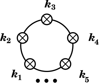
Figure 18: Leading-log contributions to $\ln Z$ at odd-loop order. Circled vertices labeled $k$ denote the insertion of the rank-$k$ induced interaction proportional to $g^{0}_{a_{1}\cdots a_{k+1}}$. For order $2p+1$ contributions, the ranks of all the insertions around the loop must sum to $p$.

The leading-log contributions at odd-loop orders are also easily determined. When the scale $\mu$ is $O(\kappa)$, so that the only source of large logarithms are the induced couplings themselves, the largest number of logarithms at a given odd loop order will result from diagrams where the maximal number of induced couplings are inserted into a graph with only one explicit loop. At loop order of $2p+1$, this means a single insertion of the rank $p$ induced coupling, or two insertions of rank $k$ and rank $p{-}k$ couplings, or more generally, the insertion of any collection of induced couplings whose ranks total $p$, as illustrated in figure 18. Rather than following the cookbook method and struggling to get the proper combinatorial factors to evaluate these diagrams, it is much easier to simply return to the original functional integral representation (3.30). The sum of the graphs in question just corresponds to the contribution of the order $\phi({\bf r})^{2}$ terms in the first line of the induced interaction (3.32) to the action

$$S^{(2)}_{\rm ind}=\Delta\kappa^{2}\,{\beta\over 2}\int(d^{\nu}{\bf r})\>\phi({\bf r})^{2}\,,$$ (6.33)

where

$$\Delta\kappa^{2}=-\sum_{p=2}^{\infty}\sum_{a_{1}\cdots a_{p}}\beta^{3p-2}\>n^{0}_{a_{1}}\cdots n^{0}_{a_{p}}\>g_{a_{1}\cdots a_{p}}\left(e_{a_{1}\cdots a_{p}}\right)^{2}\,.$$ (6.34)

Thus, the total effect of these terms is to simply shift the unperturbed (squared) Debye wave number,

$$\kappa_{0}^{2}\to\kappa^{2}_{\rm ll}\equiv\kappa_{0}^{2}+\Delta\kappa^{2}\,.$$ (6.35)

Referring back to the one-loop correction (2.79), we see the sum of these odd-loop order leading logarithms plus the original one-loop contribution is given by

$$\sum_{p=0}^{\infty}\ln Z^{(2p+1,\rm ll)}=-{\kappa_{\rm ll}^{3}\over 12\pi}\,{\cal V}\,.$$ (6.36)

A straightforward exercise expanding (6.36) and (6.34), and iterating (6.32), will yield the explicit leading-log contributions at any given order. The results up to order 6 are:

$${\ln Z^{(2,\rm ll)}\over{\cal V}} = {\cal L}\sum_{a,b}\beta^{3}\,n^{0}_{a}\,n^{0}_{b}\,e_{a}^{3}\,e_{b}^{3}\,,$$ (6.37)

$${\ln Z^{(3,\rm ll)}\over{\cal V}} = {\kappa_{0}\,{\cal L}\over 8\pi}\sum_{a,b}\beta^{4}\,n^{0}_{a}\,n^{0}_{b}\,e_{a}^{3}\,e_{b}^{3}\,(e_{a}{+}e_{b})^{2}\,,$$ (6.38)

$${\ln Z^{(4,\rm ll)}\over{\cal V}} = {\cal L}^{2}\sum_{a,b,c}\beta^{6}\,n^{0}_{a}\,n^{0}_{b}\,n^{0}_{c}\,e_{a}^{3}\,e_{b}^{3}\,e_{c}^{3}\,(e_{b}{+}e_{c})^{3}\>,$$ (6.39)

$${\ln Z^{(5,\rm ll)}\over{\cal V}} = {{\cal L}^{2}\over 32\pi\kappa_{0}}\sum_{a,b,c,d}\beta^{8}\,n^{0}_{a}\,n^{0}_{b}\,n^{0}_{c}\,n^{0}_{d}\,e_{a}^{3}\,e_{b}^{3}\,e_{c}^{3}\,e_{d}^{2}$$ (6.40)

$$\qquad\qquad\qquad{}\times\left[4(e_{b}{+}e_{c})^{3}\,(e_{a}{+}e_{b}{+}e_{c})^{2}+e_{d}\,(e_{a}{+}e_{b})^{2}\,(e_{c}{+}e_{d})^{2}\right],$$

$${\ln Z^{(6,\rm ll)}\over{\cal V}} = {{\cal L}^{3}\over 3}\sum_{a,b,c,d}\beta^{9}\,n^{0}_{a}\,n^{0}_{b}\,n^{0}_{c}\,n^{0}_{d}\,e_{a}^{3}\,e_{b}^{3}\,e_{c}^{3}\,e_{d}^{3}\,\Bigl{[}(e_{a}{+}e_{b})^{3}+2(e_{b}{+}e_{c}{+}e_{d})^{3}\Bigr{]}(e_{c}{+}e_{d})^{3}\,,$$ (6.41)

where

$${\cal L}\equiv{1\over 4!\,(4\pi)^{2}}\,\ln\!\left({\lambda^{2}\kappa^{2}\over 4\pi}\right).$$ (6.42)

The expression for the partition function in leading logarithmic orders reads

$$\ln Z^{(\rm ll)}={\cal V}\,\sum_{a=1}^{A}\,n^{0}_{a}+{\cal V}\,{\kappa_{0}^{3}\over 12\pi}+\sum_{k=2}\,\ln Z^{(k,\rm ll)}\,.$$ (6.43)

The derivatives of this form with respect to $\beta\mu_{a}$ give the leading logarithmic relations between the physical densities $\bar{n}_{a}$ and the ‘bare’ densities $n^{0}_{b}$. Solving for the bare densities in terms of the physical quantities expresses the leading-log partition function in the form

$$\ln Z^{(\rm ll)}={\cal V}\,\sum_{a=1}^{A}\,\bar{n}_{a}-{\cal V}\,{\bar{\kappa}^{3}\over 24\pi}+\sum_{k=2}\,\ln\bar{Z}^{(k,\rm ll)}\,,$$ (6.44)

in which

$${\ln\bar{Z}^{(2,\rm ll)}\over{\cal V}} = -{\cal L}\sum_{a,b}\beta^{3}\,\bar{n}_{a}\,\bar{n}_{b}\,e_{a}^{3}\,e_{b}^{3}\,,$$ (6.45)

$${\ln\bar{Z}^{(3,\rm ll)}\over{\cal V}} = -{3\,\kappa\,{\cal L}\over 8\pi}\sum_{a,b}\beta^{4}\,\bar{n}_{a}\,\bar{n}_{b}\,e_{a}^{4}\,e_{b}^{4}\,,$$ (6.46)

$${\ln\bar{Z}^{(4,\rm ll)}\over{\cal V}} = -12{\cal L}^{2}\sum_{a,b,c}\beta^{6}\,\bar{n}_{a}\,\bar{n}_{b}\,\bar{n}_{c}\,e_{a}^{3}\,e_{b}^{4}\,e_{c}^{5}\>,$$ (6.47)

$${\ln\bar{Z}^{(5,\rm ll)}\over{\cal V}} = -{5{\cal L}^{2}\over 16\pi\kappa}\sum_{a,b,c,d}\beta^{8}\,\bar{n}_{a}\,\bar{n}_{b}\,\bar{n}_{c}\,\bar{n}_{d}\,e_{a}^{2}\,e_{b}^{3}\,e_{c}^{4}\,e_{d}^{4}\left[e_{a}^{2}\,e_{b}+12e_{b}\,e_{c}\,e_{d}+16e_{b}\,e_{d}^{2}+12e_{c}\,e_{d}^{2}\right]\!,\,$$ (6.48)

$${\ln\bar{Z}^{(6,\rm ll)}\over{\cal V}} = -12{\cal L}^{3}\sum_{a,b,c,d}\beta^{9}\,\bar{n}_{a}\,\bar{n}_{b}\,\bar{n}_{c}\,\bar{n}_{d}\,e_{a}^{3}\,e_{b}^{3}\,e_{c}^{4}\,e_{d}^{5}\,$$ (6.49)

$$\kern 79.49744pt{}\times\Bigl{[}3e_{a}e_{b}e_{c}+3e_{b}^{2}e_{c}+3e_{c}^{2}e_{d}+3e_{c}e_{d}^{2}+5e_{b}e_{d}^{2}+14e_{b}e_{c}e_{d}\Bigr{]}\,.$$

Note that for even-loop orders these leading-logarithmic contributions always include a sum of particle densities weighted by an odd power of the charge. Consequently, the leading-logarithmic contributions at even-loop order vanish in the special case of a neutral symmetric binary plasma, such as a pure electron-proton plasma, where the charges of the two species are equal and opposite and the the physical densities are necessarily equal due to charge neutrality. This is a general result, which follows from the recursive structure of (6.31) and the vanishing of its initial term. The corresponding leading logarithmic expansion of the free energy $F$ is easily obtained from the thermodynamic relation $\beta\,p=\ln Z/{\cal V}=-\partial(\beta F)/\partial{\cal V}$. Using this relation, it is easy to confirm that the overall coefficients of the first three logarithmic terms, the two, three, and four loop terms, (6.45), (6.46), and (6.47), agree with the corresponding free energy terms computed by Ortner [12] and displayed in his Eq. (93). As we have noted before, Ortner works with a plasma of various species of positive ions moving in a fixed background of neutralizing negative charge. This model allows him to use a purely classical description, in which the effective short-distance cutoff is provided by the essential singularities of the Boltzmann factors with purely repulsive Coulomb interactions. Thus, as was explained before in the discussion of Eq. (5.32), the quantum length $\lambda$ in the argument of the logarithm in Eq. (6.42) is replaced by the Coulomb length $d_{C}=\beta\,e^{2}/(4\pi)$ in Ortner’s results.

6.3 “Anomalous” Virial Relation

The grand canonical partition function may be regarded as a function of the temperature and the (bare) density $n^{0}_{a}$, charge $e_{a}$, and thermal wavelength $\lambda_{a}$ of each species. If one defines an average density $n$ which is the geometric mean of the bare densities $n^{0}_{a}$ and thus entails $\beta^{-3/2}$ times the exponential of the average of the chemical potentials, then one may alternatively express a specific density in terms of the average density and a relative density ratio $x_{a}$,

$$n^{0}_{a}\equiv n\,x_{a}\,.$$ (6.50)

The charges of each species may similarly be written in terms of some mean charge $e$ and a relative charge ratio $y_{a}$,

$$e_{a}\equiv e\,y_{a}\,.$$ (6.51)

Any dependence on the thermal wavelength $\lambda_{a}$ may be re-expressed as dependence on the dimensionless quantum parameter $\eta_{a}=\beta e_{a}^{2}/4\pi\lambda_{a}$. Consequently, any $n$-loop contribution will equal $(\beta e^{2}\kappa_{0})^{n}$ times some function of the dimensionless variables $\{x_{a}\}$, $\{y_{a}\}$ and $\{\eta_{a}\}$. This is a precise version of the statement that the loop expansion parameter (in the physical limit of three dimensions) is $\beta e^{2}\kappa_{0}$. The point to be emphasized is that the parameter $\beta e^{2}\kappa_{0}$ captures the overall powers of the inverse temperature, charge, and densities that appear in a given loop order. Therefore, the grand canonical partition function has the functional form

$$\ln Z={\cal F}(\beta e^{2}\kappa_{0},x,y,\eta)\left({\cal V}\,{\sum}_{b}n_{b}^{0}\right).$$ (6.52)

Let us pretend, for the moment, that ${\cal F}$ does not depend on the quantum parameters $\eta_{a}$ — or that the purely classical theory exists. We note that the differential operator $\left[\beta{\partial\over\partial\beta}-{\textstyle{3\over 2}}\sum_{a}{\partial\over\partial\beta\mu_{a}}\right]$ annihilates the density ratios $x_{a}$, the charge ratios $y_{a}$, and also $\beta e^{2}\kappa_{0}$ because

$$\left[\beta{\partial\over\partial\beta}-{3\over 2}{\sum}_{a}{\partial\over\partial\beta\mu_{a}}\right]\beta^{2}e^{4}\kappa_{0}^{2}\sim\left[\beta{\partial\over\partial\beta}-{3\over 2}{\sum}_{a}{\partial\over\partial\beta\mu_{a}}\right]\beta^{3/2}{\sum}_{b}e^{\beta\mu_{b}}=0\,.$$ (6.53)

Since

$$\left[\beta{\partial\over\partial\beta}-{3\over 2}{\sum}_{a}{\partial\over\partial\beta\mu_{a}}\right]n_{b}^{0}=-3\,n_{b}^{0}\,,$$ (6.54)

this shows that

$$\left[3+\beta{\partial\over\partial\beta}-{3\over 2}{\sum}_{a}{\partial\over\partial\beta\mu_{a}}\right]{\cal F}(\beta e^{2}\kappa_{0},x,y)\left({\cal V}{\sum}_{b}n_{b}^{0}\right)=0\,.$$ (6.55)

In other words, a purely classical partition function must satisfy

$$\left[3+\beta{\partial\over\partial\beta}-{3\over 2}{\sum}_{a}{\partial\over\partial\beta\mu_{a}}\right]\ln Z=0\,.$$ (6.56)

Recalling that the pressure $p$ appears as

$$\ln Z[\mu]=\beta\,p\,{\cal V}\,,$$ (6.57)

the thermodynamic, internal energy density $u$ is given by

$$-{\partial\ln Z[\mu]\over\partial\beta}=u{\cal V}\,,$$ (6.58)

and the number density $\bar{n}_{a}$ of species $a$ by

$${\partial\ln Z[\mu]\over\partial\beta\mu_{a}}=\bar{n}_{a}{\cal V}\,,$$ (6.59)

the identity (6.56) for a purely classical plasma is equivalent to the relation

$$3\beta p-\beta u-{3\over 2}\,{\sum}_{a}\bar{n}_{a}=0\,.$$ (6.60)

Of course, the purely classical plasma (with oppositely charged particles) does not exist. The induced couplings necessary to render the theory finite give rise to additional dependence on the quantum parameters $\eta_{a}$. Hence, in fact,

$$A\equiv 3\beta p-\beta u-{3\over 2}\,{\sum}_{a}\bar{n}_{a}\neq 0\,.$$ (6.61)

The non-vanishing of $A$ arises from the ‘anomalous’ dependence on the underlying quantum physics. This behavior shows that $A$ is akin to the anomalies encountered in relativistic quantum field theories.

To find an expression for the anomaly $A$, which may be evaluated without separately computing the pressure, internal energy, and densities, we turn to the functional integral representation of the grand canonical partition function. It proves convenient for this specific application to use a scaled potential $\tilde{\phi}({\bf r})=\beta\phi({\bf r})$ so that the interaction terms now involve

$$n_{a}^{0}\,e^{ie_{a}\beta\phi}=n_{a}^{0}\,e^{ie_{a}\tilde{\phi}}\,,$$ (6.62)

with no explicit appearance of the inverse temperature $\beta$ (although it does reside in the densities $n_{a}^{0}$). Thus the functional integral takes the form

$$Z[\mu]={\rm Det}^{1/2}\left[-\beta^{-1}\nabla^{2}\right]\int[d\tilde{\phi}]\>\exp\left\{-{1\over 2\beta}\int(d^{\nu}{\bf r})\>\left(\nabla\tilde{\phi}({\bf r})\right)^{2}-S_{\rm int}[\tilde{\phi};\mu]\right\}\,.$$ (6.63)

Although the method that we shall outline is valid for $S_{\rm int}[\tilde{\phi};\mu]$ taken to arbitrary order, to keep the notation simple, we shall consider only those pieces that contribute to the three-loop order to which we have calculated,

$$S_{\rm int}[\tilde{\phi};\mu] = \int(d^{\nu}{\bf r})\>\biggl{[}-\sum_{a}n^{0}_{a}\,e^{ie_{a}\tilde{\phi}({\bf r})}+\sum_{a,b}g^{0}_{ab}\,\beta^{3}\,n_{a}^{0}\,e^{ie_{a}\tilde{\phi}({\bf r})}\,n_{b}^{0}\,e^{ie_{b}\tilde{\phi}({\bf r})}$$ (6.64)

$$\qquad\qquad-\sum_{a}\,h^{0}_{a}\,\beta^{2}\,e_{a}^{2}\,\left(\nabla\tilde{\phi}({\bf r})\right)^{2}n_{a}^{0}\,e^{ie_{a}\tilde{\phi}({\bf r})}+\cdots\>\biggr{]}\,.$$

We shall first find an expression for the pressure using its identification with the response to a change in the volume,

$$\delta\ln Z[\mu]=\beta\,p\>\delta{\cal V}\,,$$ (6.65)

with the change in volume realized by a dilation transformation of the spatial coordinates within the functional integral. To do this in a conceptually simple way, we temporarily introduce general coordinates $x^{k}$ and a metric tensor $g_{kl}$, so that the physical distance between neighboring points is given by

$$ds^{2}=\sum_{k,l=1}^{\nu}g_{kl}\>dx^{k}dx^{l}\,.$$ (6.66)

The $(\nabla\tilde{\phi})^{2}$ part of the action in the functional integral now takes on the generally covariant form

$$\int(d^{\nu}x)\>\sqrt{\det g}\>g^{kl}\,\partial_{k}\tilde{\phi}(x)\partial_{l}\tilde{\phi}(x)\,\left[{1\over 2\beta}-\sum_{a}\,h^{0}_{a}\,\beta^{2}\,e_{a}^{2}\,n_{a}^{0}\,e^{ie_{a}\tilde{\phi}(x)}\right]\,.$$ (6.67)

For the terms in $S_{\rm int}$ which do not involve derivatives, the introduction of generalized coordinates is effected by simply including the factor $\sqrt{\det g}$ in the spatial integration measure. To effect a dilation or scale change, we take

$$g_{kl}=e^{2\sigma}\delta_{kl}\,.$$ (6.68)

In view of the distance interval (6.66), this has the effect of the length alteration $L\to Le^{\sigma}$. With this metric, the determinantal factor and inverse metric are simply

$$\sqrt{\det g}=e^{\nu\sigma}\,,\qquad g^{kl}=e^{-2\sigma}\delta_{kl}\,.$$ (6.69)

Finally, taking the constant parameter $\sigma$ to be infinitesimal, $\sigma\to\delta\sigma$, we have a volume change $\delta{\cal V}=\nu\,\delta\sigma{\cal V}$. Thus, the variation of the functional integral (6.63) brought about by the volume change in the pressure definition (6.65) gives

$$\nu\beta p = -(\nu{-}2)\,\left<\!\left<\left(\nabla\tilde{\phi}\right)^{2}\left[{1\over 2\beta}-\sum_{a}\,h^{0}_{a}\,\beta^{2}\,e^{2}_{a}\,n_{a}^{0}\,e^{ie_{a}\tilde{\phi}}\right]\right>\!\right>$$ (6.70)

$$\qquad+\nu\left<\!\left<\sum_{a}n^{0}_{a}\,e^{ie_{a}\tilde{\phi}}-\sum_{a,b}g^{0}_{ab}\,\beta^{3}\,n_{a}^{0}\,e^{ie_{a}\tilde{\phi}}\,n_{b}^{0}\,e^{ie_{b}\tilde{\phi}}\right>\!\right>\,.$$

Using the functional integral representation (6.63) to evaluate the definitions (6.58) and (6.59) of the energy and particle number yields

$$-\beta u{\cal V}={1\over 2\beta}\left<\!\left<\left(\nabla\tilde{\phi}\right)^{2}\right>\!\right>{\cal V}-\left<\!\left<\beta{\partial\over\partial\beta}\,S_{\rm int}[\tilde{\phi};\mu]\right>\!\right>\,.$$ (6.71)

and

$$-{\sum}_{a}\bar{n}_{a}{\cal V}={\sum}_{a}\left<\!\left<{\partial\over\partial\beta\mu_{a}}\,S_{\rm int}[\tilde{\phi};\mu]\right>\!\right>\,.$$ (6.72)

Since each of the quantities that make up the anomaly (6.61) is well defined, we may write it as a $\nu\to 3$ limit in a form that will prove to be convenient,

$$A=\nu\beta p-\beta u-{\nu\over 2}\,{\sum}_{a}\bar{n}_{a}\,.$$ (6.73)

The results above express this as

$$A = \left<\!\left<(3{-}\nu){1\over 2\beta}\left(\nabla\tilde{\phi}\right)^{2}+\left[\nu-2+\beta{\partial\over\partial\beta}-{\nu\over 2}\,{\sum}_{c}{\partial\over\partial\beta\mu_{c}}\right]\sum_{a}\,h^{0}_{a}\,\beta^{2}\,e^{2}_{a}\,\left(\nabla\tilde{\phi}\right)^{2}\,n_{a}^{0}\,e^{ie_{a}\tilde{\phi}}\right>\!\right>$$ (6.74)

$$+\left<\!\left<\left[\nu+\beta{\partial\over\partial\beta}-{\nu\over 2}\,{\sum}_{c}{\partial\over\partial\beta\mu_{c}}\right]\left\{\sum_{a}n^{0}_{a}\,e^{ie_{a}\tilde{\phi}}-\sum_{a,b}g^{0}_{ab}\,\beta^{3}\,n_{a}^{0}\,e^{ie_{a}\tilde{\phi}}\,n_{b}^{0}\,e^{ie_{b}\tilde{\phi}}\right\}\right>\!\right>\,.$$

The commutation relation

$$\left[\nu+\beta{\partial\over\partial\beta}-{\nu\over 2}\,{\sum}_{c}{\partial\over\partial\beta\mu_{c}}\right]n_{a}^{0}=n_{a}^{0}\left[\beta{\partial\over\partial\beta}-{\nu\over 2}\,{\sum}_{c}{\partial\over\partial\beta\mu_{c}}\right].$$ (6.75)

implies that the classical action part of $S_{\rm int}$, proportional to $\sum_{a}n^{0}_{a}\,e^{ie_{a}\tilde{\phi}}$, does not contribute to the anomaly $A$ (as required). Moreover,

$$\left[\beta{\partial\over\partial\beta}-{\nu\over 2}\,{\sum}_{c}{\partial\over\partial\beta\mu_{c}}\right]\beta^{3}\,n_{b}^{0}=\beta^{3}\,n_{b}^{0}\left[(3{-}\nu)+\beta{\partial\over\partial\beta}-{\nu\over 2}\,{\sum}_{c}{\partial\over\partial\beta\mu_{c}}\right].$$ (6.76)

Hence we have, to our three-loop order of accuracy,

$$A = \left<\!\left<(3{-}\nu){1\over 2\beta}\left(\nabla\tilde{\phi}\right)^{2}+\sum_{a}\,\beta^{3}\,{\partial h^{0}_{a}\over\partial\beta}\,e_{a}^{2}\,n_{a}^{0}\,\left(\nabla\tilde{\phi}\right)^{2}\,e^{ie_{a}\tilde{\phi}}\right>\!\right>$$ (6.77)

$$-\sum_{ab}\left[\left((3{-}\nu)+\beta{\partial\over\partial\beta}\right)g^{0}_{ab}\right]\beta^{3}\,\left<\!\left<n_{a}^{0}\,e^{ie_{a}\tilde{\phi}}n_{b}^{0}\,e^{ie_{b}\tilde{\phi}}\right>\!\right>\,.$$

To compute the two and three loop contributions to the anomaly $A$, we first note that since to these orders the number densities are given by

$$\bar{n}_{a}=n_{a}^{0}\left<\!\left<e^{ie_{a}\tilde{\phi}}\right>\!\right>+h^{0}_{a}\,\beta^{2}\,e^{2}_{a}\,n_{a}^{0}\,\left<\!\left<\left(\nabla\tilde{\phi}\right)^{2}e^{ie_{a}\tilde{\phi}}\right>\!\right>-2\sum_{b}\beta^{3}\,g^{0}_{ab}\,n_{a}^{0}\,n_{b}^{0}\left<\!\left<e^{ie_{a}\tilde{\phi}}e^{ie_{b}\tilde{\phi}}\right>\!\right>\,,$$ (6.78)

we may write the pressure (6.70) as

$$\nu\beta p = -(\nu{-}2){1\over 2\beta}\left<\!\left<\left(\nabla\tilde{\phi}\right)^{2}\right>\!\right>+\sum_{a}\left[\nu\bar{n}_{a}+2\,e_{a}^{2}\,n^{0}_{a}\,h^{0}_{a}\,\beta^{2}\,\left<\!\left<\left(\nabla\tilde{\phi}\right)^{2}e^{ie_{a}\tilde{\phi}}\right>\!\right>\right]$$ (6.79)

$$\qquad\qquad+\nu\sum_{a,b}\beta^{3}\,g^{0}_{ab}\,n_{a}^{0}\,n_{b}^{0}\left<\!\left<e^{ie_{a}\tilde{\phi}}e^{ie_{b}\tilde{\phi}}\right>\!\right>\,.$$

The pressure and densities are, of course, well defined in the $\nu\to 3$ limit. Hence, in the above expression, the pole in $\nu{-}3$ in the final term, coming from $g^{0}_{ab}$, must be canceled by a similar pole, with opposite residue, in $\left<\!\left<(\nabla\tilde{\phi})^{2}\right>\!\right>$. Since the contribution of the coupling $h^{0}_{a}$ has a coefficient that is already of two-loop order, to the order to which we work,

$$\lim_{\nu\to 3}\>(3{-}\nu)\,{1\over 2\beta}\left<\!\left<\left(\nabla\tilde{\phi}\right)^{2}\right>\!\right>=3\sum_{a,b}\beta^{3}\left[\lim_{\nu\to 3}\>(3{-}\nu)\,g^{0}_{ab}\right]n_{a}^{0}\,n_{b}^{0}\left<\!\left<e^{ie_{a}\tilde{\phi}}e^{ie_{b}\tilde{\phi}}\right>\!\right>\,.$$ (6.80)

Recalling the result (6.1) for $g^{0}_{ab}$, we have

$$\lim_{\nu\to 3}\>(3{-}\nu)\,g^{0}_{ab}=-{1\over 4!}\,{(e_{a}e_{b})^{3}\over(4\pi)^{2}}\,.$$ (6.81)

Since $\lambda_{ab}^{2}\sim\beta$, Eq’s. (6.3), (6.4), and (3.82) also inform us that, in the $\nu\to 3$ limit,

$$\beta\,{\partial g^{0}_{ab}\over\partial\beta}=-{1\over 4!}\,{(e_{a}e_{b})^{3}\over(4\pi)^{2}}\left[1+{\textstyle{1\over 2}}\,\eta_{ab}\,\Gamma^{\prime}_{ab}\right]\,,$$ (6.82)

where $\Gamma^{\prime}_{ab}\equiv d\Gamma_{ab}/d\eta_{ab}$ is given in Eq. (4.19). Finally, Eq. (3.33) gives

$$\beta^{3}{\partial\over\partial\beta}h_{a}^{0}=-{\lambda_{a}^{2}\over 48\pi}\,.$$ (6.83)

Thus, reverting to the conventionally normalized field $\phi$, and discarding terms of higher order,

$$A = -{1\over 4!}\sum_{a,b}\beta^{3}\,n_{a}^{0}\,n_{b}^{0}\>{(e_{a}e_{b})^{3}\over(4\pi)^{2}}\,\left<\!\left<\exp\left\{i\beta\left(e_{a}+e_{b}\right)\phi({\bf r})\right\}\right>\!\right>\Big{[}3-2-{\textstyle{1\over 2}}\,\eta_{ab}\,\Gamma^{\prime}_{ab}\Big{]}$$ (6.84)

$$\qquad\qquad-\sum_{a}{\lambda_{a}^{2}\over 48\pi}\,e_{a}^{2}\,\beta^{2}\,n_{a}^{0}\left<\!\left<\left(\nabla\phi\right)^{2}\right>\!\right>\,.$$

In the last line we use the result (5.7),

$$\beta\,\left<\!\left<\left(\nabla\phi\right)^{2}\right>\!\right>={\kappa^{3}\over 4\pi}\,.$$ (6.85)

For the remaining terms, we expand the exponential involving $\phi$ to second order to generate the sub-leading (three loop) contribution. It involves, in the physical $\nu\to 3$ limit

$$\beta\left<\!\left<\phi^{2}\right>\!\right>=\lim_{\nu\to 3}G_{\nu}({\bf 0})=-{\kappa_{0}\over 4\pi}\,.$$ (6.86)

Expanding $(e_{a}{+}e_{b})^{2}$, the terms involving $e_{a}^{2}$ and $e_{b}^{2}$ just provide the one-loop corrections that alter the bare densities $n_{a}^{0}$ and $n_{a}^{0}$ to the physical densities $\bar{n}_{a}$ and $\bar{n}_{b}$. Hence, only the cross term provides a non-trivial correction, and we have

$$A = -{1\over 4!}{1\over(4\pi)^{2}}\sum_{a,b}\bar{n}_{a}\,\bar{n}_{b}\,(\beta\,e_{a}e_{b})^{3}\,\Big{[}1-{\textstyle{1\over 2}}\,\eta_{ab}\,\Gamma^{\prime}_{ab}\Big{]}\left(1+{\beta\,e_{a}e_{b}\,\bar{\kappa}\over 4\pi}\right)$$ (6.87)

$$\qquad\qquad-\sum_{a}{\lambda_{a}^{2}\kappa^{2}\over 48\pi}\,{\beta e_{a}^{2}\kappa\over 4\pi}\,\bar{n}_{a}\,.$$

This agrees with Eq. (5.23).

7 Long Distance Correlations

Figure 19: Correction to the irreducible density-density correlator $C_{ab}$ generated by the induced interaction $S_{\rm non-static}$ involving the non-zero frequency modes of $\phi({\bf r},\tau)$. The dashed lines represent the long-range, unscreened Coulomb Green’s functions of the non-zero frequency modes.

As noted in section III, the interaction (3.93) which couples the static and non-zero frequency modes of the electrostatic potential only affects thermodynamic quantities at six-loop order. However, this term does generate some qualitatively new effects in correlation functions. In particular, it destroys the exponential screening of the quasi-classical theory [14, 15, 16]. This effect is easy to calculate using the effective theory as given in Eq’s. (3.92) and (3.93).

We will first examine the workings of this effect on the single-particle irreducible part $C_{ab}({\bf r}{-}{\bf r}^{\prime})$ of the number density correlation function. The graph of Fig. 19 is produced if each of the variational derivatives in the definition (3.35) of the number density correlator act on $S_{\rm non-static}$ in the functional integral (3.92). The non-zero-frequency potentials that this brings down from the exponential become tied together into the product of two unscreened, long-ranged Coulomb Green’s functions. Since the result is single-particle irreducible, it defines an $O\left[(\beta e^{2}\kappa)(\kappa\lambda)^{4}\right]$ correction to $C_{ab}({\bf r}{-}{\bf r}^{\prime})$. Explicitly, the calculation that we have just described gives the long-ranged contribution

$$\Delta C_{ab}({\bf r}{-}{\bf r}^{\prime})={1\over(4\pi)^{2}}\>n_{a}\,n_{b}\,e_{a}^{2}\,e_{b}^{2}\,\lambda_{a}^{2}\,\lambda_{b}^{2}\>\,\beta^{2}\sum_{m\neq 0}{2\over(2\pi m)^{4}}\,\Bigl{[}\nabla_{k}\nabla_{l}V_{C}({\bf r}{-}{\bf r}^{\prime})\Bigr{]}^{2}\,.$$ (7.1)

Here

$$\sum_{m\neq 0}{2\over(2\pi m)^{4}}={\zeta(4)\over 4\pi^{4}}={1\over 360}\,,$$ (7.2)

and

$$\Bigl{[}\nabla_{k}\nabla_{l}V_{C}({\bf r}{-}{\bf r}^{\prime})\Bigr{]}^{2}={6\over(4\pi)^{2}\,|{\bf r}{-}{\bf r}^{\prime}|^{6}}\,,$$ (7.3)

and so

$$\Delta C_{ab}({\bf r}{-}{\bf r}^{\prime})={1\over 60}\,{(\beta\,e_{a}^{2}\,n_{a}\,\lambda_{a}^{2})\,(\beta\,e_{b}^{2}\,n_{b}\,\lambda_{b}^{2})\over(4\pi)^{4}\,|{\bf r}{-}{\bf r}^{\prime}|^{6}}\,.$$ (7.4)

Consequently, density-density correlations do not, in fact, decay exponentially but rather have long-distance $1/r^{6}$ tails.

We may use the relation given in Eq. (2.108) connecting the electrostatic Green’s function ${\cal G}({\bf r}{-}{\bf r}^{\prime})=\left<\!\left<\phi({\bf r})\phi({\bf r}^{\prime})\right>\!\right>$ and $C_{ab}$,

$$\beta\,\tilde{\cal G}({\bf k})=\biggl{[}k^{2}+\beta\sum_{a,b}e_{a}e_{b}\,\tilde{C}_{ab}({\bf k})\biggr{]}^{-1}\,,$$ (7.5)

to find the long-distance tail in ${\cal G}({\bf r}{-}{\bf r})$. Treating $\Delta C_{ab}({\bf r}{-}{\bf r}^{\prime})$ as a perturbation and noting that the long-distance limit of the unperturbed Green’s function is given by the Debye screened function, we have

$$\beta\Delta{\cal G}({\bf r}{-}{\bf r}^{\prime})=-\int(d^{3}{\bf r}_{1})(d^{3}{\bf r}_{2})\>{e^{-\kappa|{\bf r}{-}{\bf r}_{1}|}\over 4\pi|{\bf r}{-}{\bf r}_{1}|}\>\beta\sum_{a,b}e_{a}e_{b}\Delta C_{ab}({\bf r}_{1}{-}{\bf r}_{2})\,{e^{-\kappa|{\bf r}_{2}{-}{\bf r}^{\prime}|}\over 4\pi|{\bf r}_{2}{-}{\bf r}^{\prime}|}\,.$$ (7.6)

Since the flanking Debye Green’s functions that appear here are of short range, to obtain the long-distance behavior of $\beta\Delta{\cal G}({\bf r}{-}{\bf r}^{\prime})$ we may replace $\Delta C_{ab}({\bf r}_{1}{-}{\bf r}_{2})$ by $\Delta C_{ab}({\bf r}{-}{\bf r}^{\prime})$ and use

$$\tilde{G}({\bf 0})=\int(d^{3}{\bf r})\>{e^{-\kappa r}\over 4\pi r}={1\over\kappa^{2}}$$ (7.7)

to find that the potential correlator also acquires a $1/r^{6}$ tail,

$$\Delta{\cal G}({\bf r}{-}{\bf r}^{\prime})\sim-{1\over 60}\,\sum_{a,b}\>{(\beta\,e_{a}^{3}\,n_{a}\,\lambda_{a}^{2})\,(\beta\,e_{b}^{3}\,n_{b}\,\lambda_{b}^{2})\over(4\pi\kappa)^{4}\,|{\bf r}{-}{\bf r}^{\prime}|^{6}}\,.$$ (7.8)

Comparing the magnitude of this $1/r^{6}$ tail to the original $e^{-\kappa r}/4\pi r$ Debye potential, one finds that the cross-over from exponential to power-law decay occurs at the parametric scale

$$\kappa r\sim-\ln\!\left[(\lambda\kappa)^{4}(\beta e^{2}\kappa)\right].$$ (7.9)

This characterizes the number of $e$-foldings over which exponential Debye screening could, in principle, be observed before the power-law tail takes over.

The function $C_{ab}({\bf r}{-}{\bf r}^{\prime})$ describes the ‘single-particle’ irreducible part of the density-density correlation function. The (Fourier transform) of the complete correlator is given, according to Eq. (2.110), by

$$\tilde{K}_{ab}({\bf k})=\tilde{C}_{ab}({\bf k})-\left[\beta{\sum}_{c}e_{c}\tilde{C}_{ca}({\bf k})\right]\,\tilde{\cal G}({\bf k})\,\left[\beta{\sum}_{c}e_{c}\tilde{C}_{cb}({\bf k})\right].$$ (7.10)

Recalling [Eq. (2.103)] that $C_{ab}({\bf k})=\delta_{ab}\,n_{a}$ in lowest order, and employing the reasoning just used to find the long-distance behavior of the potential correlator, we see that the leading long-distance behavior of the complete density-density correlation function is given by

$$K_{ab}({\bf r}{-}{\bf r}^{\prime}) \sim \Delta C_{ab}({\bf r}{-}{\bf r}^{\prime})-\beta e_{a}n_{a}\,\Delta\tilde{\cal G}({\bf r}{-}{\bf r}^{\prime})\,\beta e_{b}n_{b}$$ (7.11)

$$-{\sum}_{c}\left[\Delta C_{ac}({\bf r}{-}{\bf r}^{\prime})\,e_{c}\,{1\over\kappa^{2}}\,\beta e_{b}n_{b}+\beta e_{a}n_{a}{1\over\kappa^{2}}\,e_{c}\,\Delta C_{cb}({\bf r}{-}{\bf r}^{\prime})\right],$$

or

$$K_{ab}({\bf r}{-}{\bf r}^{\prime})\sim{1\over 60}\,{\beta^{2}\over(4\pi)^{4}\,|{\bf r}-{\bf r}^{\prime}|^{6}}\>\sum_{cd}\left[\delta_{ac}-{\beta e_{a}\,n_{a}\,e_{c}\over\kappa^{2}}\right]\left[\delta_{bd}-{\beta e_{b}\,n_{b}\,e_{d}\over\kappa^{2}}\right](e^{2}_{c}\,n_{c}\,\lambda^{2}_{c})\,(e^{2}_{d}\,n_{d}\,\lambda^{2}_{d})\,.$$

(7.12)

The square brackets appearing in (7.12) function as projection operators into the subspace orthogonal to the charge vector $\{e_{a}\}$. Hence, the number-density—charge-density correlator constructed from this result by multiplying by $e_{b}$ and summing over $b$ (or multiplying by $e_{a}$ and summing over $a$) vanishes. Consequently, the number-density—charge-density correlation function must vanish more rapidly than $1/r^{6}$ at large distances. The leading behavior is obtained by returning to the general forms (7.10) and (7.5) to write

$${\sum}_{b}\,\tilde{K}_{ab}({\bf k})\,e_{b}=k^{2}\,\left[\beta\,{\sum}_{c}\,e_{c}\,\tilde{C}_{ca}({\bf k})\right]\,\tilde{\cal G}({\bf k})\,.$$ (7.13)

Again using the same reasoning to secure the asymptotic form, with the factor of $k^{2}$ in the Fourier transform becoming $-\nabla^{2}$ in the spatial form, gives

$${\sum}_{b}\,e_{b}\,K_{ab}({\bf r}{-}{\bf r}^{\prime})\sim-{1\over 2}{\beta^{2}\over(4\pi)^{4}\,\kappa^{2}\,|{\bf r}-{\bf r}^{\prime}|^{8}}\>\sum_{cd}\left[\delta_{ac}-{\beta e_{a}\,n_{a}\,e_{c}\over\kappa^{2}}\right](e^{2}_{c}\,n_{c}\,\lambda^{2}_{c})\,(e^{3}_{d}\,\lambda^{2}_{d}\,n_{d})\,.$$ (7.14)

The charge-density—charge-density correlation function $K({\bf r}{-}{\bf r}^{\prime})$ formed from this result (by multiplying by $e_{a}$ and summing over $a$) again vanishes. The charge-density—charge-density correlator again vanishes more rapidly at infinity. This final correlation function may be obtained by multiplying Eq. (7.13) by $e_{a}$ and summing over $a$. The result is equivalent to the previous relation Eq. (3.18), and we find that the charge-density—charge-density correlator $K({\bf r}{-}{\bf r}^{\prime})$ acquires a $1/r^{10}$ tail,

$$K({\bf r}{-}{\bf r}^{\prime})\sim{28\over|{\bf r}-{\bf r}^{\prime}|^{10}}\,\left[{\sum}_{a}\>{\beta\,e_{a}^{3}\,n_{a}\,\lambda_{a}^{2}\over(4\pi)^{2}\,\kappa^{2}}\right]^{2}$$ (7.15)

When specialized to the case of a one-component plasma in the presence of a constant neutralizing background, Eq. (7.15) becomes

$$K({\bf r})\sim 28\,{e^{2}\over(4\pi)^{4}}\,{\lambda^{4}\over r^{10}}={7e^{2}\over(4\pi)^{2}}\left({\beta\hbar^{2}\over m}\right)^{2}{1\over r^{10}}\,.$$ (7.16)

The asymptotic results (7.12), (7.14), and (7.15) for the correlation functions agree with the results of the calculations of Cornu and Martin [16] and Cornu [17]. Note that, once the appropriate effective field theory is constructed, the single key result (7.4) is obtained in only a few lines.

The fact that the charge-density–particle-density correlators fall off as $1/r^{8}$, or two powers of $r$ faster than the $1/r^{6}$ tail of the potential correlator ${\cal G}$, and that the charge-density—charge-density correlator falls off yet faster by another two powers, is a direct consequence of the Poisson equation $i\nabla^{2}\phi({\bf r})=\rho({\bf r})$ relating the charge density and electrostatic potential. The positive overall sign of the asymptotic charge-charge correlator (7.15) reflects the fact that a charge fluctuation of a given sign will attract oppositely charged particles and repel similarly charged particles. Therefore, the long-distance tail of the charge-charge correlator shows a positive correlation. Essentially the same argument may also be used to confirm the overall sign of the charge-density—number-density correlator (7.14). If the charge $e_{a}$ of species $a$ is arbitrarily small (so that it is, in effect, a test charge), then Eq. (7.14) becomes

$${\sum}_{b}\,e_{b}\,K_{ab}({\bf r}{-}{\bf r}^{\prime})\sim{1\over 2}{\beta\,n_{a}\,e_{a}\over|{\bf r}-{\bf r}^{\prime}|^{8}}\>\left[{\sum}_{c}\>{\beta\,e_{c}^{3}\,n_{c}\,\lambda_{c}^{2}\over(4\pi)^{2}\,\kappa^{2}}\right]^{2}+O(e_{a}^{2}),$$ (7.17)

showing that, in linear response, a test charge of species $a$ creates an induced charge density whose long-distance tail is positively correlated with the sign of the test charge.

It should be emphasized that the above results for long distance tails were derived for zero-frequency correlator functions. One may wish to consider equal-time correlators instead. The difference between the two is determined by the behavior of non-zero frequency correlations. If $K_{ab}({\bf r},\omega_{n})$ denotes the density-density correlator at spatial separation ${\bf r}$ and (Matsubara) frequency $\omega_{n}$, then the equal-time density-density correlator is

$$K_{ab}({\bf r},t{=}0)={1\over\beta}\,\sum_{n}K_{ab}({\bf r},\omega_{n})\,,$$ (7.18)

which differs from the zero-frequency correlator $K_{ab}({\bf r})=\beta^{-1}\,K_{ab}({\bf r},\omega{=}0)$ by the sum over all non-zero frequency components,

$$K_{ab}({\bf r},t{=}0)-K_{ab}({\bf r})=\sum_{n\neq 0}\beta^{-1}\,K_{ab}({\bf r},\omega_{n})\,.$$ (7.19)

However, these non-zero frequency number density correlation functions decrease with increasing spatial separation faster than the zero frequency correlation (7.12), and consequently the equal-time and zero-frequency correlators have the same leading long distance behavior. To understand the long-distance behavior of the non-zero frequency correlators, it is convenient to begin with the definition of the correlation function at (Matsubara) frequency $\omega_{m}$ as a second variational derivative with respect to the $m$’th Fourier component of the (time-dependent) chemical potentials,

$$\beta^{-1}\,K_{ab}({\bf r}{-}{\bf r}^{\prime},\omega_{m}) \equiv {\delta^{2}\ln Z\over\delta\beta\mu_{a}^{m}({\bf r})\>\delta\beta\mu_{b}^{-m}({\bf r}^{\prime})}$$ (7.20)

$$= \left<\!\left<{\delta S_{\rm non-static}\over\delta\beta\mu_{a}^{m}({\bf r})}{\delta S_{\rm non-static}\over\delta\beta\mu_{b}^{-m}({\bf r}^{\prime})}\right>\!\right>-\left<\!\left<{\delta^{2}S_{\rm non-static}\over\delta\beta\mu_{a}^{m}({\bf r})\>\delta\beta\mu_{b}^{-m}({\bf r}^{\prime})}\right>\!\right>\,.$$

Figure 20: Contributions to the non-zero frequency components of the density-density correlator $K_{ab}({\bf r}{-}{\bf r}^{\prime},\omega_{m})$. Dashed lines represent long-range, unscreened propagator ${\cal G}_{m}$ of non-zero frequency modes, while solid lines represent the zero-frequency propagator ${\cal G}$. Some non-zero Matsubara frequency $\omega_{m}$ flows in at the vertex labeled ${\bf r}$ and out at ${\bf r}^{\prime}$. The dashed lines in diagrams (a) and (b) must carry frequency $\omega_{m}$; in diagrams (c) and (d) the non-zero frequencies carried by each of the internal lines must sum to $\omega_{m}$.

The leading terms of $S_{\rm non-static}$ are shown in Eq. (3.93) and further corrections are presented in Eq. (B.54). The resulting tree-level, one-loop, and multi-loop contributions are illustrated schematically in Fig. 20. Determining the long-distance behavior of each contribution is straightforward by regarding ${\bf r}$ and ${\bf r}^{\prime}$ as arbitrarily far apart and evaluating each diagram in coordinate/frequency space. The leading long distance behavior is determined by the minimal number of propagators which run from the vicinity of ${\bf r}$ to near ${\bf r}^{\prime}$, together with the minimal number of spatial derivatives which act on these propagators. As noted in Eq. (3.95)] of section 3, each non-zero frequency propagator is given by

$${\cal G}_{m}({\bf r},{\bf r}^{\prime})=\langle\phi^{m}({\bf r})\phi^{-m}({\bf r}^{\prime})\rangle={1\over 4\pi\beta\,|{\bf r}-{\bf r}^{\prime}|}\,.$$ (7.21)

However, the structure of $S_{\rm non-static}$ (or ultimately, the gauge invariance of the underlying quantum theory) requires that only the gradient $\nabla\phi^{m}$ of the non-zero frequency components of $\phi$ appear in the effective theory. Consequently, each non-zero frequency propagator ${\cal G}_{m}({\bf r},{\bf r}^{\prime})$ will be acted upon, on either end, by one or more spatial derivatives, and so each non-zero frequency propagator which runs from near ${\bf r}$ to near ${\bf r}^{\prime}$ will contribute a factor which decreases at least as fast as $|{\bf r}{-}{\bf r}^{\prime}|^{-3}$ to the result. Taking account of the earlier discussion of Eq. (7.8), the zero frequency propagator ${\cal G}({\bf r}{-}{\bf r}^{\prime})$ shows exponential Debye screening out to the cross-over distance (7.9), beyond which it falls off like $|{\bf r}{-}{\bf r}^{\prime}|^{-6}$. Furthermore, the contribution of every diagram will also contain at least one overall gradient with respect to ${\bf r}$, and one with respect to ${\bf r}^{\prime}$, coming from the fact that the variational derivatives in Eq (7.20) can only act on gradients of the (non-zero frequency components of the) chemical potential appearing in Eq. (3.93) [augmented by Eq. (B.54)]. Therefore, diagrams in which $k$ non-zero frequency propagators, and $l$ zero frequency propagators run from (a neighborhood of) ${\bf r}$ to (a neighborhood of) ${\bf r}^{\prime}$ will have long distance behavior which falls at least as fast as $|{\bf r}{-}{\bf r}^{\prime}|^{-3k-6l-2}$.

If $k$ is even, the fall-off must actually be at least two powers faster. This is because such contributions can only come from terms in $S_{\rm non-static}$ which have an odd number of factors of $\nabla(\mu_{a}^{m}+ie_{a}\phi^{m})$. Such terms must actually involve at least one more derivative acting on these fields, since rotation invariance implies that only even numbers of gradients can appear in any term in the action. This is shown explicitly in the final term shown in Eq. (B.54). Consequently, in these diagrams the long range propagators are acted upon by at least one more derivative on either end of the diagram.

Since the total frequency $\omega_{m}$ flowing through each diagram is, by assumption, non-zero, every diagram must have at least one non-zero frequency propagator crossing from ${\bf r}$ to ${\bf r}^{\prime}$. But in any single-particle reducible contribution where only a single non-zero frequency propagator crosses from ${\bf r}$ to ${\bf r}^{\prime}$, such as diagram (a) of Fig. 20, the gradients appearing in the non-static action (3.93) necessarily generate Laplacians acting on either end of the propagator so the net contribution is only a local contact term proportional to $\nabla^{2}\delta({\bf r}{-}{\bf r}^{\prime})$. Consequently, single particle reducible diagrams such as (a) do not contribute at all to the long-distance behavior. Diagram (b) containing one zero-frequency, and one non-zero frequency propagator running from ${\bf r}$ to ${\bf r}^{\prime}$ has $|{\bf r}{-}{\bf r}^{\prime}|^{-11}$ long-distance behavior, while diagram (c), with two long-distance non-zero frequency propagators, has $|{\bf r}{-}{\bf r}^{\prime}|^{-10}$ fall-off, since there must be a total of eight spatial derivatives acting on the two non-zero frequency propagators. Multi-loop diagrams, such as (d), with three or more long-distance propagators, necessarily decrease like $|{\bf r}{-}{\bf r}^{\prime}|^{-11}$ or faster (up to possible logarithmic factors).

Therefore, the leading long-distance behavior of the irreducible part $C_{ab}({\bf r}{-}{\bf r}^{\prime},\omega_{m})$ of the non-zero frequency number-density correlation function is generated by diagram (c), and is order $|{\bf r}{-}{\bf r}^{\prime}|^{-10}$. A simple computation using the vertex (B.57) presented in Appendix B, together with the non-zero frequency propagator (7.21), shows that diagram (c) represents the contribution

$$\Delta C_{ab}({\bf r},\omega_{m}) = \beta^{3}\,n_{a}\,n_{b}\left[{\lambda_{a}^{4}e_{a}^{2}\over(2\pi)^{3}}\right]\left[{\lambda_{b}^{4}e_{b}^{2}\over(2\pi)^{3}}\right]H(\omega_{m})\left(\nabla_{k}\nabla_{l}\nabla_{k^{\prime}}\nabla_{l^{\prime}}\,{1\over r}\right)\!\left(\nabla_{k}\nabla_{l}\nabla_{k^{\prime}}\nabla_{l^{\prime}}\,{1\over r}\right),$$ (7.22)

where

$$H(\omega_{m}) \equiv {1\over(2\pi)^{8}}\sum_{\textstyle{n=-\infty\atop n\neq 0,m}}^{\infty}\,{1\over 2m^{4}\,n^{2}\,(m{-}n)^{2}}={1\over(2\pi)^{8}}\left[{\pi^{2}\over 3\,m^{6}}-{3\over m^{8}}\right]$$ (7.23)

$$= {1\over 12}\,(\beta\omega_{m})^{-6}-3\,(\beta\omega_{m})^{-8}\,.$$

With the (continuing) neglect of delta function terms which do not affect the long-range tail,

$$\left(\nabla_{k}\nabla_{l}\nabla_{k^{\prime}}\nabla_{l^{\prime}}\,{1\over r}\right)\left(\nabla_{k}\nabla_{l}\nabla_{k^{\prime}}\nabla_{l^{\prime}}\,{1\over r}\right) \to {3\cdot 5\cdot 7\over r^{9}}\,\,r_{l^{\prime}}\,r_{k^{\prime}}\,r_{l}\,r_{k}\,\nabla_{k}\nabla_{l}\nabla_{k^{\prime}}\nabla_{l^{\prime}}\,{1\over r}$$ (7.24)

$$= {3\cdot 5\cdot 7\over r^{10}}\>4!\,,$$

where in the last equality repeated use was made of the dimension-counting properties of the Euler operator, namely ${\bf r}\cdot\nabla\,r^{-n}=-n\,r^{-n}$. Thus

$$\Delta C_{ab}({\bf r},\omega_{m})=\beta^{3}\,{n_{a}\,n_{b}\over r^{10}}\left[{\lambda_{a}^{4}e_{a}^{2}\over(2\pi)^{3}}\right]\left[{\lambda_{b}^{4}e_{b}^{2}\over(2\pi)^{3}}\right]3\cdot 5\cdot 7\cdot 4!\>H(\omega_{m})\,.$$ (7.25)

This result for the long-range tail of the irreducible, non-zero frequency density-density correlator neglects additional corrections involving higher powers of $1/r$, and relative corrections to the coefficient of the $r^{-10}$ tail which are suppressed by further powers of the loop expansion parameter $\beta e^{2}\kappa$ (or equivalently $\kappa\lambda$).

The Fourier transform of the result (7.25) gives

$$\Delta\tilde{C}_{ab}({\bf k},\omega_{m})=|{\bf k}|^{7}\,{n_{a}\,n_{b}}\,{\beta^{3}\over 2}\left[{\lambda_{a}^{4}e_{a}^{2}\over(4\pi)^{2}}\right]\left[{\lambda_{b}^{4}e_{b}^{2}\over(4\pi)^{2}}\right]H(\omega_{m})\,.\qquad\hbox{($m\neq 0$)}$$ (7.26)

Note that this result involves the non-analytic term $|{\bf k}|^{7}=(k^{2})^{3}\,\sqrt{k^{2}}$. The action (3.93) for the non-zero frequency modes gives the lowest order, analytic contribution to the irreducible correlation function,

$$\tilde{C}_{ab}^{(0)}({\bf k},\omega_{m})=\delta_{ab}\,\beta\,{n_{a}\lambda_{a}^{2}\over 2\pi}\,{{\bf k}^{2}\over(2\pi m)^{2}}\,.\kern 119.24506pt\hbox{($m\neq 0$)}$$ (7.27)

Using the exact relation (A.50) of Appendix A, and the same type of analysis employed above, the result (7.26) for the irreducible correlator may be converted into corresponding results for the long distance behavior, at non-zero frequency, of the full number-density—number-density correlator $\tilde{K}_{ab}({\bf k},\omega_{m})$. It is easy to check that the leading non-analytic part of the single-particle reducible contribution to $\tilde{K}_{ab}({\bf k},\omega_{m})$, the second set of terms in Eq. (A.50), is also of order $|{\bf k}|^{7}$, and thus gives an additional contribution to the $1/r^{10}$ tail. However, these contributions always involve at least one extra factor of $\tilde{C}_{ac}^{(0)}({\bf k},\omega_{m})\,(e_{c}e_{d}/{\bf k}^{2})$ which is a correction of relative order $\beta e^{2}\,n\,\lambda^{2}\sim(\kappa\lambda)^{2}$, or two powers of the loop expansion parameter. Hence this correction has the same size as terms that have already been omitted in the calculation of the irreducible part of the correlator, and thus to our leading order, the complete correlator at non-zero frequency has the same long distance behavior as its irreducible part,

$$K_{ab}({\bf r},\omega_{m})\sim\Delta C_{ab}({\bf r},\omega_{m})\sim{315\over 8}\,{\beta^{3}\over r^{10}}\left[{n_{a}\lambda_{a}^{4}e_{a}^{2}\over\pi^{3}}\right]\left[{n_{b}\lambda_{b}^{4}e_{b}^{2}\over\pi^{3}}\right]H(\omega_{m})\,.$$ (7.28)

Since the non-zero frequency number-density—number-density correlator (7.28) falls faster than the zero-frequency component (7.12), this shows that the equal-time and zero-frequency number density correlators have the same long distance behavior. This is equally true for the charge-density—number-density correlator (7.14). But, from Eq. (7.28), the charge-density—charge-density correlator $K({\bf r},\omega_{m})=\sum_{a,b}e_{a}e_{b}\,K_{ab}({\bf r},\omega_{m})$ has a $1/r^{10}$ tail at non-zero frequency,

$$K({\bf r},\omega_{m})\sim{315\over 8}\,{\beta^{3}\over r^{10}}\left[{\sum}_{a}{n_{a}\,\lambda_{a}^{4}\,e_{a}^{3}\over\pi^{3}}\right]^{2}H(\omega_{m})\,,$$ (7.29)

just like its zero-frequency counterpart (7.15). However, the size of the non-zero frequency tail (7.29) is a factor of $(\lambda\kappa)^{4}$ smaller than the zero-frequency tail (7.15). Consequently, the equal time and zero-frequency charge-density—charge-density correlators have the same long distance behavior up to relative corrections suppressed by four powers of the loop expansion parameter.

When specialized to the case of a one-component plasma, the expression (7.26) for the leading non-analytic piece of the irreducible correlator at non-zero frequency agrees to leading order with the corresponding result of Cornu and Martin [16]. [We have made no effort to retain further corrections to the $|{\bf k}^{7}|$ coefficient, some of which are included in the result (3.25) of [16], which are higher order in our expansion parameter $\kappa\lambda$.]

Appendix A Functional Methods

In this Appendix, we define, in the context of our plasma theory, the generating function of connected correlation functions and its Legendre transform, the effective action. We review relevant properties of these functionals that are well known in quantum field theory, and then describe how number densities and density–density correlation functions are related to them. In particular, we show how the density-density correlator may be expressed in terms of a “single-particle irreducible” function in a way that explicitly exhibits its structure, particularly its small wave-number behavior. We also show how the mean-square fluctuations in energy, and particle numbers, may be expressed in terms of the same single-particle irreducible functions. This formalism is applied to compute the number densities, density–density correlators, and equation of state to two loop order in an particularly efficient manner in a final appendix so as to illustrate methods complimentary to those employed in the text.

The partition function of our theory, in either its original quantum form (3.6), or re-expressed as an effective theory (3.92), has a functional integral representation

$$Z[\mu]=N\int[d\phi]\>\exp\left\{-S[\phi;\mu]\right\},$$ (A.1)

where $[d\phi]$ denotes functional integration over a space and time dependent potential $\phi({\bf r},\tau)$ which is periodic, $\phi({\bf r},\beta)=\phi({\bf r},0)$. The action $S[\phi;\mu]$ has the form

$$S[\phi;\mu]={1\over 2}\int_{0}^{\beta}d\tau\int(d^{\nu}{\bf r})\>\bigl{[}\nabla\phi({\bf r},\tau)\bigr{]}^{2}+S_{\rm int}[\phi;\mu]\,.$$ (A.2)

In the original quantum theory the interaction part of the action $S_{\rm int}$ is (minus the logarithm of) the functional integral over all charged fields,

$$\exp\left\{-S_{\rm int}[\phi;\mu]\right\}=\prod_{a}\int[d\psi_{a}^{*}\,d\psi_{a}]\>\exp\biggl{\{}-\int_{0}^{\beta}d\tau\int(d^{\nu}{\bf r})\>{\cal L}_{a}\biggr{\}}\,,$$ (A.3)

with ${\cal L}_{a}$ the charged field Lagrangian defined in (3.90), but with the chemical potentials now extended to be functions of imaginary time as well as space, $\mu_{a}({\bf r})\to mu_{a}(x)=\mu_{a}({\bf r},\tau)$. In the effective theory, $S_{\rm int}$ is the sum of the classical interaction and the various induced interactions,

$$S_{\rm int}[\phi;\mu]=-\beta\int(d^{\nu}{\bf r})\>\sum_{a}n^{0}_{a}\,e^{i\beta e_{a}\phi^{0}}+S_{\rm ind}[\phi^{0};\mu]+S_{\rm non-static}[\phi^{0},\phi^{m};\mu]\,,$$ (A.4)

with $S_{\rm ind}$ and $S_{\rm non-static}$ given in Eq’s. (3.32) and (3.93), respectively, and $\{\phi^{m}({\bf r})\}$ denoting the Fourier components of $\phi({\bf r},\tau)$, as defined in Eq. (3.26).

In the following formal discussion, we will allow the generalized chemical potentials $\mu({\bf r},\tau)$ to vary both in space and (imaginary) time. The only feature of the interaction terms which will be relevant is the fact that $i\phi({\bf r},\tau)$ couples to the total charge density via the dependence of $S_{\rm int}[\phi;\mu]$ on the generalized chemical potentials $\mu_{a}({\bf r},\tau)$, or

$${\delta\over\delta\phi({\bf r},\tau)}\,S_{\rm int}[\phi;\mu]=i\,\sum_{a}e_{a}\,{\delta\over\delta\mu_{a}({\bf r},\tau)}\,S_{\rm int}[\phi;\mu]\,.$$ (A.5)

This is a reflection of the invariance (2.30) of the theory under the combined shifts $\phi\to\phi-ic$ and $\mu_{a}\to\mu_{a}-e_{a}c$.

In the following discussion, for notational convenience, we will use single symbols $x$, $y$, etc., to denote a (Euclidean) space-time coordinate so that, for example, $\phi(x)\equiv\phi({\bf r},\tau)$. And we will write $\int_{x}$ as shorthand for $\int_{0}^{\beta}d\tau\int(d^{\nu}{\bf r})$.

A.1 Connected Generating Functional

The addition of an external charge density or source $\sigma(x)$ coupled to the field $\phi(x)$ defines a functional $W[\sigma;\mu]$ which is the generating functional for connected $\phi$ field correlation functions — correlators whose graphical representations have no disconnected parts. The definition is

$$\exp{W[\sigma;\mu]}=\int[d\phi]\>\exp\left\{-S[\phi;\mu]+\int_{x}\>\phi(x)\,\sigma(x)\right\}.$$ (A.6)

In the presence of the source, a normalized thermal expectation value is defined by

$$\langle F[\phi]\,\rangle^{\sigma}_{\beta}=e^{-W[\sigma;\mu]}\,\int[d\phi]\>F[\phi]\,\exp\left\{-S[\phi;\mu]+\int_{x}\>\phi(x)\,\sigma(x)\right\},$$ (A.7)

and in terms of this expectation value

$${\delta W[\sigma;\mu]\over\delta\sigma(x)}=\langle\phi(x)\rangle^{\sigma}_{\beta}\,.$$ (A.8)

The insertion in the functional integrand of the functional derivative of $-S_{\rm int}[\phi;\mu]$ with respect to a generalized chemical $\mu_{a}(x)$ produces the average particle number density, up to an overall factor of $e^{W[\sigma;\mu]}$. Thus the properly normalized particle number density of species $a$ is given by

$$\langle n_{a}(x)\rangle^{\sigma}_{\beta}={\delta W[\sigma;\mu]\over\delta\mu_{a}(x)}\,.$$ (A.9)

This is the number density in the presence of both spatially (or temporally) varying chemical potentials $\mu_{b}(x)$ and the external charge density $\sigma(x)$. With the chemical potentials $\{\mu_{a}\}$ taken to be constants and $\sigma$ taken to vanish, Eq. (A.9) reduces to the constant number density $\bar{n}_{a}=\langle n_{a}\rangle_{\beta}$ of particles of species $a$. We shall denote this limit by a vertical bar with a subscript 0. Thus,

$$\bar{n}_{a}=\left.{\delta W[\sigma;\mu]\over\delta\mu_{a}(x)}\right|_{0}\,.$$ (A.10)

The total charge density in the presence of all the sources is given by

$$\langle\rho(x)\rangle^{\sigma}_{\beta}={\sum}_{a}\,e_{a}\,\langle n_{a}(x)\rangle^{\sigma}_{\beta}={\sum}_{a}\,e_{a}\,{\delta W[\sigma;\mu]\over\delta\mu_{a}(x)}\,.$$ (A.11)

The partial derivative of $W[\sigma;\mu]$ with respect to the inverse temperature defines the average energy in the presence of the source $\sigma$,

$$\langle E\rangle_{\beta}^{\sigma}=-{\partial W[\sigma;\mu]\over\partial\beta}\,.$$ (A.12)

In the limit of vanishing source and constant chemical potentials, this reduces to the thermodynamic internal energy,

$$U=\langle E\rangle_{\beta}=-\left.{\partial W[\sigma;\mu]\over\partial\beta}\right|_{0}\,.$$ (A.13)

Second variations with respect to the chemical potentials produce the number density correlation function,

$$K_{ab}(x{-}x^{\prime})=\left.{\delta^{2}W[\sigma;\mu]\over\delta\mu_{a}(x)\,\delta\mu_{b}(x^{\prime})}\right|_{0}\,.$$ (A.14)

The static correlator discussed in the text is just the time average of this space-time dependent correlator,

$$K_{ab}({\bf r}{-}{\bf r}^{\prime})=\beta^{-1}\int_{0}^{\beta}d\tau\>K_{ab}({\bf r}{-}{\bf r}^{\prime},\tau{-}\tau^{\prime})\,.$$ (A.15)

We shall also have occasion to use the $\phi$ field correlation function defined by

$${\cal G}(x{-}x^{\prime})=\left.{\delta^{2}W[\sigma;\mu]\over\delta\sigma(x)\,\delta\sigma(x^{\prime})}\right|_{0}\,.$$ (A.16)

Since the functional integral of a total functional derivative vanishes,

$$0=\int[d\phi]\,{\delta\over\delta\phi(x)}\exp\left\{-S[\phi;\mu]+\int_{y}\phi(y)\,\sigma(y)\right\},$$ (A.17)

the functional integral with an extra factor of

$${\delta S[\phi;\mu]\over\delta\phi(x)}-\sigma(x)$$ (A.18)

included in the integrand vanishes. Hence, in view of the form (A.2) of the action and the result (A.5), the expectation value of the field equation is an exact identity:

$$-\nabla^{2}\langle\phi(x)\rangle^{\sigma}_{\beta} = i\sum_{a}e_{a}{\delta W[\sigma;\mu]\over\delta\mu_{a}(x)}+\sigma(x)$$ (A.19)

$$= i\langle\rho(x)\rangle^{\sigma}_{\beta}+\sigma(x)\,.$$

A.2 Effective Action

The effective action functional $\Gamma[\bar{\phi};\mu]$ is defined by a Legendre transform of the generating functional $W[\sigma;\mu]$. It generalizes the mean field theory described in Sec. 2.2 to include the effects of thermal and quantum fluctuations. The effective action functional has two important properties: Not only does it contain only connected graphs (as does $W$), it contains no single-particle reducible graphs — graphs which can be cut into two disjoint pieces by cutting a single line. This is shown explicitly to two-loop order in Appendix G.2 below. This property simplifies calculations. For example, when $\Gamma$ is used to compute the free energy, one can simply delete all “tadpole” graphs. Moreover, as we shall see, the use of the effective action together with the functional relations that we are developing reveals the basic structure of the theory in a very useful form. The effective action functional is obtained by setting

$$\langle\phi(x)\rangle^{\sigma}_{\beta}=\bar{\phi}(x)\,,$$ (A.20)

that is, by considering the field expectation value rather than the source to be the independent variable. The effective action is then defined by the Legendre transformation

$$\Gamma[\bar{\phi};\mu]\equiv\int_{x}\sigma(x)\,\bar{\phi}(x)-W[\sigma;\mu]\,.$$ (A.21)

Because of Eq’s. (A.8), (A.9), and (A.12),

$$\delta\Gamma[\bar{\phi};\mu]=\int_{x}\left\{\sigma(x)\,\delta\bar{\phi}(x)-\langle n_{a}(x)\rangle^{\sigma}_{\beta}\,\delta\mu_{a}(x)\right\}+\langle E\rangle_{\beta}^{\sigma}\>d\beta\,.$$ (A.22)

Thus we may consider $\Gamma$ to be a functional of the independent variables $\bar{\phi}(x)$, $\mu_{a}(x)$, and $\beta$, with the (partial) functional derivatives

$${\delta\Gamma[\bar{\phi};\mu]\over\delta\bar{\phi}(x)}=\sigma(x)\,,$$ (A.23)

$$-{\delta\Gamma[\bar{\phi};\mu]\over\delta\mu_{a}(x)}=\langle n_{a}(x)\rangle^{\sigma}_{\beta}\,,$$ (A.24)

and the ordinary partial derivative

$${\partial\Gamma[\bar{\phi};\mu]\over\partial\beta}=\langle E\rangle^{\sigma}_{\beta}\,.$$ (A.25)

In view of Eq. (A.23), evaluating the effective action at a stationary point, a point where $\delta\Gamma/\delta\bar{\phi}=0$, is the same as setting the source $\sigma$ to zero. With constant chemical potentials and a vanishing source, the last equalities reduce to the ordinary number density and internal energy. As remarked in the text, the grand canonical partition function is related to the grand potential by $Z=\exp\{-\beta\Omega\}$, and so the grand potential is given by the effective action evaluated at its stationary point in the limit of constant chemical potentials,

$$\beta\Omega=\left.\Gamma[\bar{\phi};\mu]\right|_{0}\,.$$ (A.26)

We return momentarily to consider $\sigma(x)$ and $\mu_{a}(x)$ as independent variables so as to compute the source functional derivative of Eq. (A.23):

$$\int_{y}{\delta^{2}\Gamma[\bar{\phi};\mu]\over\delta\bar{\phi}(x)\,\delta\bar{\phi}(y)}{\delta\bar{\phi}(y)\over\delta\sigma(x^{\prime})}=\delta(x{-}x^{\prime})\,,$$ (A.27)

or, in view of Eq. (A.8),

$$\int_{y}{\delta^{2}\Gamma[\bar{\phi};\mu]\over\delta\bar{\phi}(x)\,\delta\bar{\phi}(y)}\,{\delta^{2}W[\sigma;\mu]\over\delta\sigma(y)\,\delta\sigma(x^{\prime})}=\delta(x{-}x^{\prime})\,.$$ (A.28)

In the limit of constant chemical potentials and a vanishing source, this becomes

$$\int_{y}\left.{\delta^{2}\Gamma[\bar{\phi};\mu]\over\delta\bar{\phi}(x)\,\delta\bar{\phi}(y)}\right|_{0}{\cal G}(y{-}x^{\prime})=\delta(x{-}x^{\prime})\,.$$ (A.29)

Thus

$$\left.{\delta^{2}\Gamma[\bar{\phi};\mu]\over\delta\bar{\phi}(x)\,\delta\bar{\phi}(x^{\prime})}\right|_{0}={\cal G}^{-1}(x{-}x^{\prime})$$ (A.30)

is the operator inverse to the potential correlation function ${\cal G}(x{-}x^{\prime})$. After a Fourier transform [in space and (periodic) time],

$$\tilde{\cal G}({\bf k},\omega_{m})\equiv\int_{0}^{\beta}d\tau\int(d^{\nu}{\bf r})\>e^{-i\omega_{m}\tau+i{\bf k}\cdot{\bf r}}\,{\cal G}({\bf r},\tau)\,,$$ (A.31)

the linear integral equation (A.29) reduces to the algebraic relation:

$$\tilde{\cal G}^{-1}({\bf k},\omega_{m})\,\tilde{\cal G}({\bf k},\omega_{m})=1\,.$$ (A.32)

To uncover the structure of the potential correlation function, we first write the field equation (A.19) for the expectation value in terms of the effective action functional. This is done by using Eq’s. (A.20), (A.23), and (A.24), to obtain

$$-\nabla^{2}\bar{\phi}(x)=-i\sum_{a}\,e_{a}\,{\delta\Gamma[\bar{\phi};\mu]\over\delta\mu_{a}(x)}+{\delta\Gamma[\bar{\phi};\mu]\over\delta\bar{\phi}(x)}\,.$$ (A.33)

Taking the functional derivative of this relation with respect to $\bar{\phi}(x^{\prime})$ and then setting the chemical potentials constant and the source to zero produces

$$-\nabla^{2}\delta(x{-}x^{\prime})=-i\sum_{a}e_{a}\gamma_{a}(x{-}x^{\prime})+{\cal G}^{-1}(x{-}x^{\prime})\,,$$ (A.34)

where we have defined a two-point vertex or coupling by

$$\gamma_{a}(x{-}x^{\prime})\equiv\left.{\delta^{2}\Gamma\over\delta\mu_{a}(x)\,\delta\bar{\phi}(x^{\prime})}\right|_{0}\,.$$ (A.35)

Thus in wave number/frequency space

$$\tilde{\cal G}^{-1}({\bf k},\omega_{m})={\bf k}^{2}+i\,{\sum}_{a}\,e_{a}\,\tilde{\gamma}_{a}({\bf k},\omega_{m})\,.$$ (A.36)

The structure of the potential correlation function is intimately connected to that of the number density correlation function. Hence it is useful to examine the relationship between the effective action and the number density correlator. Recalling the expression (A.14) for this function in terms of $W[\sigma;\mu]$ and then the fact [Eq. (A.9)] that one functional derivative defines the number density, we see that we may write

$$K_{ab}(x{-}x^{\prime})=\left.{\delta\over\delta\mu_{b}(x^{\prime})}\,\langle n_{a}(x)\rangle^{\sigma}_{\beta}\right|_{0}\,.$$ (A.37)

In this equation, $\sigma$ and $\mu_{a}$ are taken to be the independent variables, with $\bar{\phi}$ a function of these independent variables. Thus, using Eq. (A.24) to express the number density in terms of the effective action, we obtain

$$K_{ab}(x{-}x^{\prime})=-\left.{\delta^{2}\Gamma\over\delta\mu_{a}(x)\,\delta\mu_{b}(x^{\prime})}\right|_{0}-\left.\int_{y}{\delta^{2}\Gamma\over\delta\mu_{a}(x)\,\delta\bar{\phi}(y)}\,{\delta\bar{\phi}(y)\over\delta\mu_{b}(x^{\prime})}\right|_{0}\,.$$ (A.38)

We define

$$C_{ab}(x{-}x^{\prime})\equiv-\left.{\delta^{2}\Gamma\over\delta\mu_{a}(x)\,\delta\mu_{b}(x^{\prime})}\right|_{0}\,,$$ (A.39)

and recall the definition (A.35) to write Eq. (A.38) as

$$K_{ab}(x{-}x^{\prime})=C_{ab}(x{-}x^{\prime})-\left.\int_{y}\gamma_{a}(x{-}y)\,{\delta\bar{\phi}(y)\over\delta\mu_{b}(x^{\prime})}\right|_{0}\,.$$ (A.40)

To deal with the final variational derivative which appears here, we note that with $\sigma$ and the $\mu_{a}$ taken to be the independent variables,

$${\delta\sigma(z)\over\delta\mu_{b}(x^{\prime})}=0\,,$$ (A.41)

and so Eq. (A.23) implies that

$${\delta^{2}\Gamma\over\delta\mu_{b}(x^{\prime})\,\delta\bar{\phi}(z)}+\int_{y}{\delta\bar{\phi}(y)\over\delta\mu_{b}(x^{\prime})}\,{\delta^{2}\Gamma\over\delta\bar{\phi}(y)\,\delta\bar{\phi}(z)}=0\,.$$ (A.42)

In the limit of constant chemical potentials and vanishing source, the first term here is just $\gamma_{b}(x^{\prime}{-}z)$ and the second factor in the integrand is ${\cal G}^{-1}(y{-}z)$. Hence

$$\left.{\delta\bar{\phi}(y)\over\delta\mu_{b}(x^{\prime})}\right|_{0}=-\int_{z}{\cal G}(y{-}z)\,\gamma_{b}(x^{\prime}{-}z)\,,$$ (A.43)

and Eq. (A.40) becomes

$$K_{ab}(x{-}x^{\prime})=C_{ab}(x{-}x^{\prime})+\int_{y,z}\gamma_{a}(x{-}y)\,{\cal G}(y{-}z)\,\gamma_{b}(x^{\prime}{-}z)\,,$$ (A.44)

or, in wave number/frequency space,

$$\tilde{K}_{ab}({\bf k},\omega_{m})=\tilde{C}_{ab}({\bf k},\omega_{m})+\tilde{\gamma}_{a}({\bf k},\omega_{m})\,\tilde{\cal G}({\bf k},\omega_{m})\,\tilde{\gamma}_{b}({\bf k},\omega_{m})\,.$$ (A.45)

Since the function $\tilde{C}_{ab}({\bf k},\omega_{m})$ is a double variational derivative of the effective action functional $\Gamma[\bar{\phi};\mu_{a}]$, it is single-particle irreducible. On the other hand, $\tilde{\cal G}({\bf k},\omega_{m})$, the potential correlation function, is not single-particle irreducible.

We have yet to express the number density and potential correlation functions in the simplest terms. To do so, we return to the expectation of the field equation (A.19). With $\mu_{a}$ and $\sigma$ taken to be independent variables, the functional derivative of this equation with respect to a generalized chemical potential, with the chemical potentials then set constant and the source to zero, gives

$$\left.-\nabla^{2}{\delta\bar{\phi}(x)\over\delta\mu_{b}(x^{\prime})}\right|_{0}=i\sum_{a}e_{a}\,K_{ab}(x{-}x^{\prime})\,.$$ (A.46)

With the use of Eq’s. (A.43) and (A.45), the Fourier transform of this constraint may be put in the form

$$-\left[{\bf k}^{2}+i\,{\sum}_{a}\,e_{a}\,\tilde{\gamma}_{a}({\bf k},\omega_{m})\right]\tilde{\cal G}({\bf k},\omega_{m})\,\tilde{\gamma}_{b}({\bf k},\omega_{m})=i\,{\sum}_{a}\,e_{a}\,\tilde{C}_{ab}({\bf k},\omega_{m})\,.$$ (A.47)

The factor in square brackets on the left-hand side of this result is, according to Eq. (A.36), just ${\cal G}^{-1}({\bf k},\omega_{m})$. Hence,

$$\tilde{\gamma}_{b}({\bf k},\omega_{m})=-i\,\sum_{a}\,e_{a}\tilde{C}_{ab}({\bf k},\omega_{m})\,.$$ (A.48)

Accordingly,

$${\cal G}^{-1}({\bf k},\omega_{m})={\bf k}^{2}+\sum_{a,b}e_{a}e_{b}\,\tilde{C}_{ab}({\bf k},\omega_{m})\,,$$ (A.49)

and

$$\tilde{K}_{ab}({\bf k},\omega_{m})=\tilde{C}_{ab}({\bf k},\omega_{m})-\left[{\sum}_{c}e_{c}\,\tilde{C}_{ca}({\bf k},\omega_{m})\right]\,\tilde{\cal G}({\bf k},\omega_{m})\,\left[{\sum}_{c}e_{c}\,\tilde{C}_{cb}({\bf k},\omega_{m})\right].$$ (A.50)

We have found that both the potential and number density correlation functions are determined by the single-particle irreducible function $\tilde{C}_{ab}({\bf k},\omega_{m})$. We should note that the definition (A.39) of this function, plus rotation and time reversal invariance, implies the symmetry

$$\tilde{C}_{ab}({\bf k},\omega_{m})=\tilde{C}_{ba}({\bf k},\omega_{m})$$ (A.51)

which thus carries over to the number density correlation function $\tilde{K}_{ab}({\bf k},\omega_{m})$.

The above results may also be used to reveal the structure of correlation functions involving the charge density. The correlation function of the charge density with the number density of species $a$ is given by

$$\sum_{b}\tilde{K}_{ab}({\bf k},\omega_{m})\,e_{b} = \sum_{b}\tilde{C}_{ab}({\bf k},\omega_{m})\,e_{b}\left\{1-\tilde{\cal G}({\bf k},\omega_{m})\,\left[{\sum}_{c,d}\,e_{c}e_{d}\,\tilde{C}_{cd}({\bf k},\omega_{m})\right]\right\}$$ (A.52)

$$= \sum_{b}\tilde{C}_{ab}({\bf k},\omega_{m})\,e_{b}\,{\bf k}^{2}\,{\cal G}({\bf k},\omega_{m})\,.$$

The ${\bf k}\to 0$ limit gives the correlator of the number density with the total charge. This vanishes, as it must for the neutral plasma. Finally, the charge density – charge density correlation function is given by

$$\tilde{K}({\bf k},\omega_{m}) = \sum_{a,b}e_{a}\,\tilde{K}_{ab}({\bf k},\omega_{m})\,e_{b}$$ (A.53)

$$= {{\bf k}^{2}\left[\sum_{a,b}\,e_{a}\,\tilde{C}_{ab}({\bf k},\omega_{m})\,e_{b}\right]\over{\bf k}^{2}+\sum_{a,b}\,e_{a}\,\tilde{C}_{ab}({\bf k},\omega_{m})\,e_{b}}\,.$$

This form exhibits explicitly the small wave number behavior

$$\tilde{K}({\bf k},\omega_{m})\sim{\bf k}^{2}\,,\qquad\hbox{as ${\bf k}\to 0$}\,.$$ (A.54)

Static correlators, which are the focus of attention in the main text, are related to the zero frequency component of the corresponding time dependent correlator functions by a factor of $\beta^{-1}$:

$$\tilde{K}_{ab}({\bf k})=\beta^{-1}\,\tilde{K}_{ab}({\bf k},0)\,,$$ (A.55)

and similarly for $\tilde{C}_{ab}({\bf k})$, $\tilde{\cal G}({\bf k})$, etc. Consequently, the static versions of Eq’s. (A.49), (A.50), (A.53), and (A.54) are

$${\cal G}^{-1}({\bf k})=\beta\,{\bf k}^{2}+\beta^{2}\sum_{a,b}e_{a}e_{b}\,\tilde{C}_{ab}({\bf k})\,,$$ (A.56)

$$\tilde{K}_{ab}({\bf k})=\tilde{C}_{ab}({\bf k})-\left[\beta\,{\sum}_{c}e_{c}\,\tilde{C}_{ca}({\bf k})\right]\,\tilde{\cal G}({\bf k})\,\left[\beta\,{\sum}_{c}e_{c}\,\tilde{C}_{cb}({\bf k})\right],$$ (A.57)

$$\tilde{K}({\bf k})={{\bf k}^{2}\left[\sum_{a,b}\,e_{a}\,\tilde{C}_{ab}({\bf k})\,e_{b}\right]\over{\bf k}^{2}+\beta\sum_{a,b}\,e_{a}\,\tilde{C}_{ab}({\bf k})\,e_{b}}\,,$$ (A.58)

and

$$\tilde{K}({\bf k})\sim\beta^{-1}\,{\bf k}^{2}\,,\qquad\hbox{as ${\bf k}\to 0$}\,.$$ (A.59)

A.3 Effective Potential, Thermodynamic Quantities

In quantum field theory, the effective potential (times the space-time volume) is defined to be the restriction of the effective action to spatially (and temporally) uniform fields. We have already remarked that the further restriction to the stationary point yields the grand potential (times $\beta$). With constant chemical potentials, the stationarity condition $\delta\Gamma/\delta\bar{\phi}=0$ is just the condition that charge neutrality hold for a given value of $\bar{\phi}$. For convenience, we will assume that physical chemical potentials are chosen such that this stationary point lies at $\bar{\phi}=0$, so that

$$\beta\Omega=\left.\Gamma[\bar{\phi};\mu]\right|_{\bar{\phi}=0}\,.$$ (A.60)

This is the function that we have computed to three loops. However, the charge neutrality constraint is never used in our computations, and so, in fact, the function $\Gamma[\bar{\phi}{=}0;\mu]$ has been calculated for arbitrary (constant) chemical potentials $\mu_{a}$. This extension of the grand potential is needed for the computation of thermodynamic average numbers and energy and for the correlators of these quantities. Just as in our previous work, to derive general relationships it is convenient temporarily to work with $\Gamma[\bar{\phi};\mu]$ for arbitrary constant $\bar{\phi}$ and $\mu_{a}$. The results of these derivations, however, will depend only upon the $\bar{\phi}=0$ functions that have been computed.

With uniform fields, Eq. (A.23) reduces to

$${\partial\Gamma(\bar{\phi};\mu)\over\partial\bar{\phi}}=\sigma\beta{\cal V}\,.$$ (A.61)

As we have remarked before, the restriction to a vanishing source, $\sigma=0$, determines

$$\bar{\phi}=\bar{\phi}(\beta,\{\beta\mu_{a}\})\,,$$ (A.62)

and inserting this value of $\bar{\phi}$ in $\Gamma$ yields the physical grand potential $\beta\Omega$. With arbitrary chemical potentials, $\bar{\phi}$ is non-vanishing so as to keep a zero charge density in the plasma. The previous expressions (A.24) and (A.25), evaluated with $\bar{\phi}$ at the stationary point (A.62), gives the physical particle numbers and energy,

$$\bar{N}_{a}=\langle n_{a}{\cal V}\rangle_{\beta}=-{\partial\Gamma(\bar{\phi};\mu)\over\partial\beta\mu_{a}}\,,$$ (A.63)

and

$$U=\bar{E}=\langle E\rangle_{\beta}={\partial\Gamma(\bar{\phi};\mu)\over\partial\beta}\,.$$ (A.64)

To obtain relations for the fluctuations of these quantities, we first need two results. The derivative of Eq. (A.61) with respect to the inverse temperature keeping $\sigma=0$ so that $\bar{\phi}$ is determined by Eq. (A.62) gives, just as in the previous analogous calculation of the chemical potential functional derivative (A.42),

$${\partial^{2}\Gamma(\bar{\phi};\mu)\over\partial\beta\,\partial\bar{\phi}}+{\cal V}\,\tilde{\cal G}^{-1}({\bf 0})\,{\partial\bar{\phi}\over\partial\beta}=0\,.$$ (A.65)

Note that, from (A.56),

$$\tilde{\cal G}^{-1}({\bf 0})=\beta^{2}\sum_{a,b}e_{a}\tilde{C}_{ab}({\bf 0})e_{b}\,,$$ (A.66)

and

$$\tilde{C}_{ab}({\bf 0})={1\over{\cal V}}\,{\partial^{2}\Gamma(\bar{\phi};\mu)\over\partial\beta\mu_{a}\,\partial\beta\mu_{b}}$$ (A.67)

may be computed directly at $\bar{\phi}=0$ with chemical potentials set to values which satisfy charge neutrality (for $\bar{\phi}=0$) after the derivatives have been performed. Thus $\tilde{C}_{ab}({\bf 0})$ can be obtained from the computation of the grand potential $\beta\Omega$. We may simply write

$$\tilde{C}_{ab}({\bf 0})=-{\partial\langle n_{a}\rangle_{\beta}\over\partial\beta\mu_{b}}=-{\partial\langle n_{b}\rangle_{\beta}\over\partial\beta\mu_{a}}\,,$$ (A.68)

where the partial derivatives are taken at constant temperature or fixed $\beta$. In a similar fashion, the derivative with respect to the inverse temperature of the charge neutrality condition

$${\sum}_{a}e_{a}{\partial\Gamma(\bar{\phi};\mu)\over\partial\beta\mu_{a}}=0$$ (A.69)

produces

$${\sum}_{a}e_{a}\left\{{\partial^{2}\Gamma(\bar{\phi};\mu)\over\partial\beta\,\partial\beta\mu_{a}}+{\partial^{2}\Gamma(\bar{\phi};\mu)\over\partial\bar{\phi}\,\partial\beta\mu_{a}}\,{\partial\bar{\phi}\over\partial\beta}\right\}=0\,.$$ (A.70)

We use Eq’s. (A.35), (A.48), and (A.66) to write this as

$${\partial\bar{\phi}\over\partial\beta}=-{i\beta\over{\cal V}}\,\tilde{\cal G}({\bf 0})\,{\sum}_{a}e_{a}{\partial^{2}\Gamma(\bar{\phi};\mu)\over\partial\beta\,\partial\beta\mu_{a}}\,.$$ (A.71)

After the derivatives in the relations above have been taken, we may again assume that the chemical potentials are chosen to give charge neutrality at $\bar{\phi}=0$.

With these results in hand, we can examine the fluctuations of energy and particle numbers. The energy fluctuations in the grand canonical ensemble are given by

$$\left\langle\left(E-\bar{E}\right)^{2}\right\rangle_{\beta} = -{\partial\over\partial\beta}{\partial\Gamma(\bar{\phi};\mu)\over\partial\beta}$$ (A.72)

$$= -{\partial^{2}\Gamma(\bar{\phi};\mu)\over\partial\beta^{2}}-{\partial^{2}\Gamma(\bar{\phi};\mu)\over\partial\beta\,\partial\bar{\phi}}\,{\partial\bar{\phi}\over\partial\beta}\,.$$

We can make use of Eq. (A.65) to write this as

$$\left\langle\left(E-\bar{E}\right)^{2}\right\rangle_{\beta}=-{\partial^{2}\Gamma(\bar{\phi};\mu)\over\partial\beta^{2}}+{\partial^{2}\Gamma(\bar{\phi};\mu)\over\partial\beta\,\partial\bar{\phi}}{1\over{\cal V}}\,\tilde{\cal G}({\bf 0}){\partial^{2}\Gamma(\bar{\phi};\mu)\over\partial\beta\,\partial\bar{\phi}}\,,$$ (A.73)

or alternatively use Eq’s. (A.65) and (A.71) to write

$$\left\langle\left(E-\bar{E}\right)^{2}\right\rangle_{\beta}=-{\partial^{2}\Gamma(\bar{\phi};\mu)\over\partial\beta^{2}}-\left[{\sum}_{a}e_{a}{\partial^{2}\Gamma(\bar{\phi};\mu)\over\partial\beta\,\partial\beta\mu_{a}}\right]{\beta^{2}\over{\cal V}}\,\tilde{\cal G}({\bf 0})\left[{\sum}_{a}e_{a}{\partial^{2}\Gamma(\bar{\phi};\mu)\over\partial\beta\,\partial\beta\mu_{a}}\right].$$ (A.74)

This latter form may be evaluated at $\bar{\phi}=0$ with the chemical potentials chosen to give charge neutrality after their derivatives have been taken. Thus, this latter form is determined by the quantities calculated for the grand potential $\beta\Omega$. The energy — particle number correlation is given by

$$\left\langle\left(E-\bar{E}\right)\left(N_{a}-\bar{N}_{a}\right)\right\rangle_{\beta}=-{\partial\bar{N}_{a}\over\partial\beta} = {\partial\over\partial\beta}{\partial\Gamma(\bar{\phi};\mu)\over\partial\beta\mu_{a}}$$ (A.75)

$$= {\partial^{2}\Gamma(\bar{\phi};\mu)\over\partial\beta\,\partial\beta\mu_{a}}+{\partial^{2}\Gamma(\bar{\phi};\mu)\over\partial\bar{\phi}\,\partial\beta\mu_{a}}\,{\partial\bar{\phi}\over\partial\beta}\,.$$

With the use of Eq’s. (A.35), (A.48), and (A.71), this becomes

$$\left\langle\left(E-\bar{E}\right)\left(N_{a}-\bar{N}_{a}\right)\right\rangle_{\beta}={\partial^{2}\Gamma(\bar{\phi};\mu)\over\partial\beta\,\partial\beta\mu_{a}}-{\sum}_{b}e_{b}{\partial^{2}\Gamma(\bar{\phi};\mu)\over\partial\beta\,\partial\beta\mu_{b}}\,\tilde{\cal G}({\bf 0})\,\beta^{2}\,{\sum}_{c}\tilde{C}_{ac}({\bf 0})e_{c}\,.$$ (A.76)

Again, this result depends only upon quantities involved in the construction of $\beta\Omega$. Note that, in view of Eq. (A.66), the charge neutrality condition is obeyed,

$${\sum}_{a}\left\langle\left(E-\bar{E}\right)\left(N_{a}-\bar{N}_{a}\right)\right\rangle_{\beta}e_{a}=0\,.$$ (A.77)

Finally, we note that the Fourier transform (A.57) evaluated at zero wave number yields the particle number — particle number correlators,

$$\left\langle\left(N_{a}-\bar{N}_{a}\right)\left(N_{b}-\bar{N}_{b}\right)\right\rangle_{\beta}={\cal V}\left\{\tilde{C}_{ab}({\bf 0})-\left[\beta{\sum}_{c}e_{c}\tilde{C}_{ca}({\bf 0})\right]\tilde{\cal G}({\bf 0})\left[\beta{\sum}_{c}e_{c}\tilde{C}_{cb}({\bf 0})\right]\right\}.$$ (A.78)

The results that we have obtained may be used to compute the specific heat at constant volume. This is simply related to the derivative of the average energy with respect to the inverse temperature at constant particle numbers,

$$C_{\rm V}=-\beta^{2}\left.{\partial\bar{E}\over\partial\beta}\right|_{\{\bar{N}_{a}\}}.$$ (A.79)

Thus the chemical potentials must change as the temperature is varied in order to maintain constant numbers. That is, we have

$$d\bar{E} = {\partial\bar{E}\over\partial\beta}\,d\beta+{\sum}_{a}{\partial\bar{E}\over\partial\beta\mu_{a}}\,d(\beta\mu_{a})$$ (A.80)

$$= \left\{{\partial^{2}\Gamma(\bar{\phi};\mu)\over\partial\beta^{2}}+\left[{\sum}_{a}e_{a}{\partial^{2}\Gamma(\bar{\phi};\mu)\over\partial\beta\,\partial\beta\mu_{a}}\right]{\beta^{2}\over{\cal V}}\,\tilde{\cal G}({\bf 0})\left[{\sum}_{a}e_{a}{\partial^{2}\Gamma(\bar{\phi};\mu)\over\partial\beta\,\partial\beta\mu_{a}}\right]\right\}d\beta$$

$${}+{\sum}_{a}\left\{{\partial^{2}\Gamma(\bar{\phi};\mu)\over\partial\beta\,\partial\beta\mu_{a}}-\left[{\sum}_{b}e_{b}{\partial^{2}\Gamma(\bar{\phi};\mu)\over\beta\,\partial\beta\mu_{b}}\right]\tilde{\cal G}({\bf 0})\beta^{2}\left[{\sum}_{c}\tilde{C}_{ac}({\bf 0})e_{c}\right]\right\}d(\beta\mu_{a})\,,$$

with the chemical potential changes constrained by

$$0 = d\bar{N}_{a}={\partial\bar{N}_{a}\over\partial\beta}\,d\beta+{\sum}_{b}{\partial\bar{N}_{a}\over\partial\beta\mu_{b}}\,d(\beta\mu_{b})$$ (A.81)

$$= -\left\{{\partial^{2}\Gamma(\bar{\phi};\mu)\over\partial\beta\,\partial\beta\mu_{a}}-\left[{\sum}_{b}e_{b}{\partial^{2}\Gamma(\bar{\phi};\mu)\over\partial\beta\,\partial\beta\mu_{b}}\right]\tilde{\cal G}({\bf 0})\beta^{2}\left[{\sum}_{c}\tilde{C}_{ac}({\bf 0})e_{c}\right]\right\}d\beta$$

$${}+{\sum}_{b}{\cal V}\left\{\tilde{C}_{ab}({\bf 0})-\left[\beta{\sum}_{c}e_{c}\tilde{C}_{ca}({\bf 0})\right]\,\tilde{\cal G}({\bf 0})\left[\beta{\sum}_{c}e_{c}\tilde{C}_{cb}({\bf 0})\right]\right\}d(\beta\mu_{b})\,.$$

Introducing the inverse matrix $\tilde{C}^{-1}({\bf 0})$,

$${\sum}_{b}\tilde{C}^{-1}({\bf 0})_{ab}\,\tilde{C}_{bc}({\bf 0})=\delta_{ac}\,,$$ (A.82)

which is a symmetric matrix since $||\tilde{C}_{ab}({\bf 0})||$ is symmetric, we may rewrite Eq. (A.81) as

$$d(\beta\mu_{a}) = {1\over{\cal V}}{\sum}_{b}\tilde{C}^{-1}({\bf 0})_{ab}{\partial^{2}\Gamma(\bar{\phi};\mu)\over\partial\beta\,\partial\beta\mu_{b}}\,d\beta$$ (A.83)

$${}-e_{a}\left\{{1\over{\cal V}}\left[{\sum}_{b}e_{b}{\partial^{2}\Gamma(\bar{\phi};\mu)\over\partial\beta\,\partial\beta\mu_{b}}\right]\tilde{\cal G}({\bf 0})\beta^{2}\,d\beta-\tilde{\cal G}({\bf 0})\,\beta^{2}\sum_{bc}e_{b}\,\tilde{C}_{bc}({\bf 0})\,d(\beta\mu_{c})\right\}.$$

Because of the charge neutrality condition (A.77), a change $d(\beta\mu_{a})$ proportional to $e_{a}$ does not alter Eq. (A.80). Hence

$$\left.{\partial\bar{E}\over\partial\beta}\right|_{\{N_{a}\}}={\partial^{2}\Gamma(\bar{\phi};\mu)\over\partial\beta^{2}}+{1\over{\cal V}}\sum_{a,b}{\partial^{2}\Gamma(\bar{\phi};\mu)\over\partial\beta\,\partial\beta\mu_{a}}\,\tilde{C}^{-1}({\bf 0})_{ab}{\partial^{2}\Gamma(\bar{\phi};\mu)\over\partial\beta\,\partial\beta\mu_{b}}\,.$$ (A.84)

A.4 Time-Dependent Correlations

We noted in section 3.6 that although the static two-point potential correlation function, the zero frequency part of the general correlator, describes a Debye screened potential (except for the very long-distance tail elucidated in section 7), the non-zero frequency parts of this correlation function are not Debye screened. Recalling the general result (A.49):

$${\cal G}^{-1}({\bf k},\omega_{m})={\bf k}^{2}+\sum_{a,b}e_{a}e_{b}\,\tilde{C}_{ab}({\bf k},\omega_{m})\,,$$ (A.85)

this lack of Debye screening for $\omega_{m}\neq 0$ is the statement that, for this case,

$${\bf k}^{2}\to 0\,:\qquad\tilde{C}_{ab}({\bf k},\omega_{m})\sim k^{2}\,,$$ (A.86)

which implies that ${\cal G}^{-1}({\bf r}-{\bf r}^{\prime},\omega_{m})$ behaves as $|{\bf r}-{\bf r}^{\prime}|^{-1}$ for large $|{\bf r}-{\bf r}^{\prime}|$. In this section we shall show how this follows from the conservation of the number currents or, equivalently, from the gauge invariance of the coupling of the basic theory to a set of [($\nu{+}1$)-dimensional] vector potentials.

Number-current correlation functions are generated by coupling a vector potential $A_{\mu}^{a}(x)\equiv(A_{4}^{a}(x),{\bf A}^{a}(x))$ for each particle species $a$. This is done by augmenting the Lagrangian (3.90) for each basic charged field to read

$${\cal L}_{a}=\psi_{a}^{*}({\bf r},\tau)\left\{{\partial\over\partial\tau}-A_{4}^{a}({\bf r},\tau)-{1\over 2m_{a}}\left[\nabla-i{\bf A}^{a}({\bf r},\tau)\right]^{2}-\mu_{a}-ie_{a}\phi({\bf r},\tau)\right\}\psi_{a}({\bf r},\tau)\,.$$ (A.87)

Connected correlation functions of $n$ space-time currents $J^{a}_{\mu}(x)\equiv(n_{a}({\bf r},\tau),{\bf J}_{a}({\bf r},\tau))$ are produced by $n$ functional derivatives $\delta/\delta A_{\mu}^{a}(x)$ acting on the generating functional $W$. In particular, the connected number-density correlation function (A.14) is now extended to the space-time correlation function

$$K_{ab}^{\mu\nu}(x{-}x^{\prime})=\left.{\delta^{2}W[\sigma;A]\over\delta A_{\mu}^{a}(x)\,\delta A_{\nu}^{b}(x^{\prime})}\right|_{0}\,.$$ (A.88)

The corresponding connected, single-particle irreducible function is given by the same functional derivatives of the Legendre transform of $W$, the effective action $\Gamma$. This extension of Eq. (A.39) reads

$$C_{ab}^{\mu\nu}(x{-}x^{\prime})=-\left.{\delta^{2}\Gamma\over\delta A_{\mu}^{a}(x)\,\delta A_{\nu}^{b}(x^{\prime})}\right|_{0}\,.$$ (A.89)

The actions formed from the extended Lagrangians (A.87) are invariant under local phase rotations of the charged fields

$$\psi_{a}^{*}(x)\to\psi_{a}^{*}(x)\exp\{-i\lambda^{a}(x)\}\,,\qquad\psi_{a}(x)\to\exp\{i\lambda^{a}(x)\}\psi_{a}(x)\,,$$ (A.90)

coupled with the gauge transformations of the external potentials

$$A_{4}^{a}(x)\to A_{4}^{a}(x)+i{\partial\lambda^{a}\over\partial\tau}\,,\qquad A_{k}^{a}(x)\to A_{k}^{a}(x)+{\partial\lambda^{a}\over\partial x^{k}}\,.$$ (A.91)

The integration measures of the charged field functional integrals are unchanged by the phase rotation (A.90). Hence the connected generating functional $W[A]$ is invariant under the gauge transformation (A.91). This invariance carries over to the effective action $\Gamma[A]$ since the Legendre transformation which relates it to $W[A]$ involves only neutral fields that are not altered by the phase rotation or gauge transformation. In the limit of an infinitesimal transformation, the gauge invariance gives functional differential statements

$$\partial_{\mu}{\delta\over\delta A_{\mu}^{a}(x)}W[A]=0=\partial_{\mu}{\delta\over\delta A_{\mu}^{a}(x)}\Gamma[A]\,,$$ (A.92)

where we have adopted the shorthand notation

$$\partial_{\mu}=\left(i{\partial\over\partial\tau}\,,{\partial\over\partial x^{k}}\right)\,.$$ (A.93)

Taking additional functional derivatives of Eq’s. (A.92) shows that any number current correlation function has a transverse form. In particular, one additional functional derivative yields

$$\partial_{\mu}K_{ab}^{\mu\nu}(x{-}x^{\prime})=0=\partial_{\nu}K_{ab}^{\mu\nu}(x{-}x^{\prime})\,,$$ (A.94)

and

$$\partial_{\mu}C_{ab}^{\mu\nu}(x{-}x^{\prime})=0=\partial_{\nu}C_{ab}^{\mu\nu}(x{-}x^{\prime})\,.$$ (A.95)

In terms of Fourier components,

$$-i\omega_{m}\,\tilde{C}_{ab}^{4\nu}({\bf k},\omega_{m})+k^{l}\,\tilde{C}_{ab}^{l\nu}({\bf k},\omega_{m})=0\,.$$ (A.96)

We are now in a position to demonstrate that the potential correlation function at non-zero frequency has no Debye screening. Three paragraphs ago, we remarked that this correlator is determined by $\tilde{C}_{ab}({\bf k},\omega_{m})=\tilde{C}_{ab}^{44}({\bf k},\omega_{m})$. Because of rotational invariance, $\tilde{C}_{ab}^{l4}({\bf k},\omega_{m})=k^{l}\,f_{ab}(k^{2},\omega_{m})$ and the $\nu=4$ component of the Fourier form (A.96) of the divergence condition becomes

$$-i\omega_{m}\,\tilde{C}_{ab}({\bf k},\omega_{m})+k^{2}\,f_{ab}(k^{2},\omega_{m})=0\,.$$ (A.97)

This demonstrates the assertion (A.86) that $\tilde{C}_{ab}({\bf k},\omega_{m})\sim k^{2}$ as $k^{2}\to 0$ when $\omega_{m}\neq 0$ and thus that there is no Debye screening in the $\omega_{m}\neq 0$ potential correlation function ${\cal G}({\bf k},\omega_{m})$.

The fact that, for small $k^{2}$, $\tilde{C}_{ab}({\bf k},\omega_{m})=O(k^{2})$ when $\omega_{m}\neq 0$ but $\tilde{C}_{ab}({\bf k},0)=O(1)$ might appear a bit odd since $\tilde{C}_{ab}({\bf k},\omega_{m})$ is equal to an analytic function of $\omega$, $F_{ab}(k^{2},\omega)$, evaluated at discrete points on the imaginary axis, $\omega=i\omega_{m}=i2\pi m/\beta$. Thus one might expect a uniform behavior in $\omega$ which would require that $\tilde{C}_{ab}({\bf k},0)=O(k^{2})$ for small $k^{2}$ and no Debye screening. In fact, the behavior of the analytic function $F_{ab}(k^{2},\omega)$ is not uniform in $k^{2}$ when $\omega$ is small. This non-uniform behavior is illustrated by the simple one-loop contribution of the charged fields to $\tilde{C}_{ab}({\bf k},\omega_{m})$. To further simplify the result, we also take the $\hbar\to$ classical limit but with the frequency $\omega_{m}/\hbar$ kept fixed to obtain

$$\tilde{C}_{ab}({\bf k},\omega_{m})=\tilde{C}_{ab}^{44}({\bf k},\omega_{m})=\delta_{ab}\int{(d^{\nu}p)\over(2\pi)^{\nu}}\>{1\over i(\omega_{m}/\hbar)-({\bf p}\cdot{\bf k}/m_{a})}\>{\bf k}\cdot{\partial\over\partial{\bf p}}n^{0}_{a}({\bf p})\,,$$ (A.98)

where

$$n^{0}_{a}({\bf p})=g_{a}\,\exp\left\{-\beta\left[{{\bf p}^{2}\over 2m_{a}}-\mu_{a}\right]\right\}$$ (A.99)

is the Maxwell-Boltzmann density of particles in momentum space. This result is obtained by taking the indicated limits of Eq. (B.40) in the following Appendix. Taking $\omega_{m}=0$ gives

$$\tilde{C}_{ab}({\bf k},O) = \delta_{ab}\int{(d^{\nu}p)\over(2\pi)^{\nu}}\>{1\over(-{\bf p}\cdot{\bf k}/m_{a})}\,(-\beta{\bf p}\cdot{\bf k}/m_{a})n^{0}_{a}({\bf p})$$ (A.100)

$$= \delta_{ab}\,\beta n^{0}_{a}\,,$$

which produces the leading order contribution to the Debye wave number,

$${\sum}_{ab}e_{a}e_{b}\tilde{C}_{ab}({\bf k},O)={\sum}_{a}\beta e^{2}_{a}n^{0}_{a}=\kappa_{0}^{2}\,,$$ (A.101)

yielding for small $k^{2}$ [c.f. Eq. (A.85)]

$${\cal G}^{-1}({\bf k},0)\approx k^{2}+\kappa^{2}_{0}\,,$$ (A.102)

On the other hand, for $\omega_{m}\neq 0$, the linear term in ${\bf k}$ in Eq. (A.98) vanishes, and expanding the denominator to first order in ${\bf k}$ together with a partial integration of ${\bf k}\cdot{\partial\over\partial{\bf p}}$ gives the small $k^{2}$ limit

$$\tilde{C}_{ab}({\bf k},\omega_{m})=\delta_{ab}\left({\hbar\over\omega_{m}}\right)^{2}\,{k^{2}\over m_{a}}\,n_{a}^{0}\,.$$ (A.103)

The corresponding small $k^{2}$ contribution to the potential correlator produces

$${\cal G}^{-1}({\bf k},\omega_{m})\approx k^{2}\left[1+{\hbar^{2}\omega_{P}^{2}\over\omega_{m}^{2}}\right]\,,$$ (A.104)

where

$$\omega_{P}^{2}={\sum}_{a}{e_{a}^{2}n^{0}_{a}\over m_{a}}$$ (A.105)

is the lowest order contribution to the plasma frequency. This is the result (3.98) given in the text.

To see how the non-uniform behavior of the one-loop correlator (A.98) is in accord with the conservation (A.96) of the number current correlators, we note that the classical limit of a one-loop calculation also gives

$$\tilde{C}_{ab}^{l4}({\bf k},\omega_{m})=\delta_{ab}\int{(d^{\nu}p)\over(2\pi)^{\nu}}\>{p^{l}\over m_{a}}\,{1\over i(\omega_{m}/\hbar)-({\bf p}\cdot{\bf k}/m_{a})}\>{\bf k}\cdot{\partial\over\partial{\bf p}}\,n^{0}_{a}({\bf p})\,.$$ (A.106)

We see that these contributions to $-i\omega_{m}\,\tilde{C}_{ab}^{44}({\bf k},\omega_{m})+k^{l}\,\tilde{C}_{ab}^{l4}({\bf k},\omega_{m})$ combine to form the integral of a total derivative which vanishes, and so the current conservation is confirmed. We also note the non-uniform limits

$$\tilde{C}_{ab}^{l4}({\bf k},0)=0\,,$$ (A.107)

while for $\omega_{m}\neq 0$,

$$k^{2}\to 0\,:\qquad\tilde{C}_{ab}^{l4}({\bf k},\omega_{m})=\delta_{ab}\,{i\hbar\over\omega_{m}}\,{n^{0}_{a}\over m_{a}}\,k^{l}\,.$$ (A.108)

For the sake of completeness, we note that the calculations leading to Eq. (A.50) are easily generalized to relate the number current correlation functions to their single-particle irreducible counterparts. The result is

$$\tilde{K}_{ab}^{\mu\nu}({\bf k},\omega_{m})=\tilde{C}_{ab}^{\mu\nu}({\bf k},\omega_{m})-\left[{\sum}_{c}e_{c}\,\tilde{C}_{ca}^{4\mu}({\bf k},\omega_{m})\right]\,\tilde{\cal G}({\bf k},\omega_{m})\,\left[{\sum}_{c}e_{c}\,\tilde{C}_{cb}^{4\nu}({\bf k},\omega_{m})\right].$$ (A.109)

We also note that time-reversal and spatial-rotation invariance together with the current conservation imply the symmetries

$$\tilde{C}_{ab}^{\mu\nu}({\bf k},\omega_{m})=\tilde{C}_{ab}^{\nu\mu}({\bf k},\omega_{m})=\tilde{C}_{ba}^{\mu\nu}({\bf k},\omega_{m})\,,$$ (A.110)

and

$$\tilde{C}_{ab}^{\mu\nu}({\bf k},\omega_{m})^{*}=\tilde{C}_{ab}^{\mu\nu}(-{\bf k},-\omega_{m})\,.$$ (A.111)

Appendix B Green’s Functions and Determinants

The result (3.6) in the text involves a product of path integrals of the form

$$Z[V]=\int[d\psi^{*}d\psi]\exp\left\{-\int_{0}^{\beta}d\tau\int(d^{\nu}{\bf r})\>\psi^{*}({\bf r},\tau)\left[{\partial\over\partial\tau}-{\nabla^{2}\over 2m}-\mu+V({\bf r},\tau)\right]\psi({\bf r},\tau)\right\},$$ (B.1)

with $m$ one of the masses $\{m_{a}\}$ and $V({\bf r},\tau)=-ie\phi({\bf r},\tau)$, with $e$ the corresponding charge $e_{a}$. When the chemical potential is generalized to contain spatial or temporal variation, so as to generate number density correlation functions, its spatially or temporally varying part will be implicitly included in the potential $V$. The field $\psi({\bf r},\tau)$ is either periodic (for Bosons) or antiperiodic (for Fermions) in $\tau$ with period $\beta$. The external potential $V({\bf r},\tau)$ is initially defined in the interval $0<\tau<\beta$, but may be extended to all real $\tau$ by regarding it as a periodic function with period $\beta$. The functional integral produces an inverse determinant in the Bose case and a determinant in the Fermi case,

$$Z[V]={\rm Det}^{\mp 1}\left[{\partial\over\partial\tau}-{\nabla^{2}\over 2m}-\mu+V({\bf r},\tau)\right].$$ (B.2)

In this appendix, we shall show how the determinant $Z[V]$ is related to a sum of ordinary, single-particle quantum-mechanical amplitudes. We shall then make use of this result to derive approximate evaluations of $Z[V]$ that become valid in the limit in which the dynamics may be treated classically, approximations that are used in the calculations of the text. These needed results could perhaps be obtained more quickly with other methods, but the development given here hopefully illuminates the character of the theory and the intermediate results that are obtained may be useful in other contexts.

The determinant can be constructed by integrating its variation. The familiar form for the variation of the determinant gives

$$\delta\ln Z[V]=\mp\int_{0}^{\beta}\int(d^{\nu}{\bf r})\>G_{\beta}({\bf r},\tau;{\bf r},\tau{+}0)\>\delta V({\bf r},\tau)\,,$$ (B.3)

in which the thermal Green’s function $G_{\beta}$ is defined by

$$\left[{\partial\over\partial\tau}-{\nabla^{2}\over 2m}-\mu+V({\bf r},\tau)\right]G_{\beta}({\bf r},\tau;{\bf r}^{\prime}\tau^{\prime})=\delta(\tau{-}\tau^{\prime})\,\delta({\bf r}{-}{\bf r}^{\prime})\,,$$ (B.4)

together with the boundary conditions that it be periodic for Bosons and antiperiodic for Fermions with a period of $\beta$,

$$G_{\beta}({\bf r},\tau{+}\beta;{\bf r}^{\prime}\tau^{\prime})=G_{\beta}({\bf r},\tau;{\bf r}^{\prime},\tau^{\prime}{+}\beta)=\pm G_{\beta}({\bf r},\tau;{\bf r}^{\prime},\tau^{\prime})\,.$$ (B.5)

The coincident time limit used in the variation (B.3), in which $\tau^{\prime}\to\tau$ from above, is needed to give the proper operator ordering $\psi^{\dagger}\psi$ that represents the density operator.

To construct the thermal Green’s function, it is convenient to introduce the quantum-mechanical transformation function in imaginary time $\langle{\bf r},\tau|{\bf r}^{\prime},\tau^{\prime}\rangle$ whose dynamics is governed by the external potential. It is defined by

$$\left[{\partial\over\partial\tau}-{\nabla^{2}\over 2m}+V({\bf r},\tau)\right]\langle{\bf r},\tau|{\bf r}^{\prime},\tau^{\prime}\rangle=0\,,$$ (B.6)

together with the boundary condition

$$\langle{\bf r},\tau|{\bf r}^{\prime},\tau\rangle=\delta({\bf r}{-}{\bf r}^{\prime})\,.$$ (B.7)

We now assert that the thermal Green’s function in the interval $-\beta\leq\tau,\tau^{\prime}\leq\beta$ has the construction (akin to an image construction in electrostatics)

$$G_{\beta}({\bf r},\tau;{\bf r}^{\prime},\tau^{\prime})=\theta(\tau{-}\tau^{\prime})\,\langle{\bf r},\tau|{\bf r}^{\prime},\tau^{\prime}\rangle+\sum_{n=1}^{\infty}(\pm 1)^{n}e^{\mu(\tau{-}\tau^{\prime}+n\beta)}\langle{\bf r},\tau{+}n\beta|{\bf r}^{\prime},\tau^{\prime}\rangle\,,$$ (B.8)

where $\theta(\tau)$ is the unit step function. The proof is as follows. Since

$$G_{\beta}({\bf r},\tau^{\prime}{+}0;{\bf r}^{\prime},\tau^{\prime})-G_{\beta}({\bf r},\tau^{\prime}{-}0;{\bf r}^{\prime},\tau^{\prime})=\langle{\bf r},\tau^{\prime}|{\bf r}^{\prime},\tau^{\prime}\rangle=\delta({\bf r}{-}{\bf r}^{\prime})\,,$$ (B.9)

Eq. (B.6) implies that the inhomogeneous Green’s function equation (B.4) is obeyed. And the construction is easily seen to satisfy the periodicity condition (B.5).

The coincident time limit of the Green’s function which enters into the variation (B.3) thus has the representation

$$G_{\beta}({\bf r},\tau;{\bf r},\tau{+}0)=\sum_{n=1}^{\infty}(\pm 1)^{n}e^{n\beta\mu}\langle{\bf r},\tau{+}n\beta|{\bf r},\tau\rangle\,.$$ (B.10)

Thus

$$\delta\ln Z[V]=-\sum_{n=1}^{\infty}(\pm 1)^{n{+}1}e^{n\beta\mu}\int_{0}^{\beta}d\tau\int(d^{\nu}{\bf r})\>\langle{\bf r},\tau{+}n\beta|{\bf r},\tau\rangle\>\delta V({\bf r},\tau)\,.$$ (B.11)

Since the potential is periodic,

$$V({\bf r},\tau+k\beta)=V({\bf r},\tau)\,,$$ (B.12)

so is the transformation function in the presence of this potential,

$$\langle{\bf r},\tau{+}k\beta{+}n\beta|{\bf r},\tau{+}k\beta\rangle=\langle{\bf r},\tau{+}n\beta|{\bf r},\tau\rangle\,.$$ (B.13)

Hence, since we may add $n$ equal copies if we divide by $n$, we may write

$$\delta\ln Z[V]=-\sum_{n=1}^{\infty}(\pm 1)^{n{+}1}{e^{n\beta\mu}\over n}\int_{0}^{n\beta}d\tau\int(d^{\nu}{\bf r})\>\langle{\bf r},\tau{+}n\beta|{\bf r},\tau\rangle\>\delta V({\bf r},\tau)\,.$$ (B.14)

To integrate this variational statement, we introduce a complete set of intermediate states and write

$$\langle{\bf r},\tau{+}n\beta|{\bf r},\tau\rangle=\int(d^{\nu}{\bf\bar{r}})\>\langle{\bf r},\tau{+}n\beta|{\bf\bar{r}},n\beta\rangle\,\langle{\bf\bar{r}},n\beta|{\bf r},\tau\rangle\,,$$ (B.15)

and again use the periodicity of the external potential to write

$$\langle{\bf r},\tau{+}n\beta|{\bf\bar{r}},n\beta\rangle=\langle{\bf r},\tau|{\bf\bar{r}},0\rangle\,.$$ (B.16)

Hence, the variational statement may be expressed as

$$\delta\ln Z[V] = -\sum_{n=1}^{\infty}(\pm 1)^{n{+}1}{e^{n\beta\mu}\over n}\int_{0}^{n\beta}d\tau\int(d^{\nu}{\bf r})(d^{\nu}{\bf\bar{r}})\>\langle{\bf\bar{r}},n\beta|{\bf r},\tau\rangle\>\delta V({\bf r},\tau)\>\langle{\bf r},\tau|{\bf\bar{r}},0\rangle$$ (B.17)

$$= \sum_{n=1}^{\infty}(\pm 1)^{n{+}1}{e^{n\beta\mu}\over n}\int(d^{\nu}{\bf\bar{r}})\>\delta\langle{\bf\bar{r}},n\beta|{\bf\bar{r}},0\rangle\,,$$

where the second equality recognizes that this is just the variation of the transformation function when the potential is varied. Hence,

$$\ln Z[V]=\sum_{n=1}^{\infty}(\pm 1)^{n{+}1}{e^{n\beta\mu}\over n}\int(d^{\nu}{\bf r})\>\langle{\bf r},n\beta|{\bf r},0\rangle\,,$$ (B.18)

which expresses the determinant in terms of an expansion in powers $n$ of the fugacity $z=e^{\beta\mu}$ whose coefficients are traces of single-particle transformation functions over the imaginary time interval $(0,n\beta)$. To confirm that the correct integration constant has been secured, we note that when the external potential $V({\bf r},\tau)$ vanishes, this form immediately gives the free-particle partition function since in this case

$$\langle{\bf r},n\beta|{\bf r},0\rangle^{0}=\int{(d^{\nu}{\bf p})\over(2\pi)^{\nu}}\>e^{-n\beta p^{2}/2m}\,,$$ (B.19)

and so

$$\ln Z[V] = \sum_{n=1}^{\infty}{(\pm 1)^{n{+}1}\over n}\,e^{n\beta\mu}\int(d^{\nu}{\bf r})\>\int{(d^{\nu}{\bf p})\over(2\pi)^{\nu}}\>e^{-n\beta p^{2}/2m}$$ (B.20)

$$= \mp\int{(d^{\nu}{\bf r})(d^{\nu}{\bf p})\over(2\pi)^{\nu}}\>\ln\left[1\mp e^{\beta\mu}e^{-\beta p^{2}/2m}\right]\,,$$

which is the well-known result for the quantum-statistical free-particle partition function.

The single-particle transformation functions that appear here have a convenient path integral representation

$$\int(d^{\nu}{\bf r})\>\langle{\bf r},n\beta|{\bf r},0\rangle=\int[d{\bf r}]\>\exp\left\{-\int_{0}^{n\beta}d\tau\left[{m\over 2}\,{d{\bf r}\over d\tau}\cdot{d{\bf r}\over d\tau}+V({\bf r}(\tau),\tau)\right]\right\}\,.$$ (B.21)

Here the functional integral is over all paths that begin and end at position ${\bf r}$, ${\bf r}(0)={\bf r}={\bf r}(n\beta)$, with ${\bf r}$ then integrated over the large spatial volume ${\cal V}\/$. In other words, the integral is over all paths which are periodic with period $n\beta\hbar$. In the limit in which the quantum-mechanical aspects of the particle’s dynamics is not important, the classical limit for the dynamics which is equivalent to the large mass $m$ limit, the dominant path is just the constant path ${\bf r}(\tau)={\bf r}$ so that, in this limit,

$$\int(d^{\nu}{\bf r})\>\langle{\bf r},n\beta|{\bf r},0\rangle=\langle{\bf r},n\beta|{\bf r},0\rangle^{0}\int(d^{\nu}{\bf r})\>\exp\left\{-n\int_{0}^{\beta}d\tau\>V({\bf r},\tau)\right\}\,,$$ (B.22)

where the overall constant is determined by the free-particle limit (B.19), and the periodicity of the potential has been used to write the integral from $0$ to $n\beta$ as $n$ times the integral from $0$ to $\beta$. Placing this approximation in the general result (B.18) gives

$$\ln Z[V]=\mp\int{(d^{\nu}{\bf r})(d^{\nu}{\bf p})\over(2\pi)^{\nu}}\>\ln\left[1\mp\exp\left\{\beta\mu-\beta{p^{2}\over 2m}-\int_{0}^{\beta}d\tau\>V({\bf r},\tau)\right\}\right]\,.$$ (B.23)

In this expression, the quantum Bose-Einstein or Fermi-Dirac statistics are treated exactly, but the dynamics is treated entirely classically. In the limit of classical statistics, $-\beta\mu\gg 1$, and only the first term in the expansion of the logarithm is significant. Replacing $V$ by $-ie\phi$ and remembering the definition of the bare particle density puts this classical limit in the form

$$\ln Z[V]=\int(d^{\nu}{\bf r})\>n^{0}\,\exp\left\{ie\int_{0}^{\beta}d\tau\>\phi({\bf r},\tau)\right\}\,.$$ (B.24)

This is the formula used in the text and derived there so as to obtain the correct Coulomb classical partition function. Here we have obtained it as the classical limit of the many-particle, quantum mechanical system.

To find sub-leading corrections to the large mass limit, it is convenient first to derive an exact series representation. The representation is obtained by placing the Fourier transform representation of the potential

$$V({\bf r},\tau)=\int{(d^{\nu}{\bf k})\over(2\pi)^{\nu}}\>\tilde{V}({\bf k},\tau)\,e^{i{\bf k}\cdot{\bf r}}$$ (B.25)

in the exponent of the functional integral (B.21) and expanding the exponential in powers of the potential. Interchanging the orders of integration then yields

$$\int(d^{\nu}{\bf r})\>\langle{\bf r},n\beta|{\bf r},0\rangle$$

$$\quad=\sum_{l=0}^{\infty}{(-1)^{l}\over l!}\int_{0}^{n\beta}d\tau_{1}\int{(d^{\nu}{\bf k}_{1})\over(2\pi)^{\nu}}\>\tilde{V}({\bf k}_{1},\tau_{1})\>\cdots\>\int_{0}^{n\beta}d\tau_{l}\int{(d^{\nu}{\bf k}_{l})\over(2\pi)^{\nu}}\>\tilde{V}({\bf k}_{l},\tau_{l})\;z_{n}[{\bf F}]\,,$$ (B.26)

in which

$$z_{n}[{\bf F}]=\int[d{\bf r}]\>\exp\left\{-\int_{0}^{n\beta}d\tau\left[{m\over 2}\,{d{\bf r}\over d\tau}\cdot{d{\bf r}\over d\tau}+{\bf F}(\tau)\cdot{\bf r}(\tau)\right]\right\},$$ (B.27)

with

$${\bf F}(\tau)=-i\sum_{a=1}^{l}\>{\bf k}_{a}\,\delta(\tau{-}\tau_{a})\,.$$ (B.28)

The remaining path integral (B.27) describes free-particle motion (in imaginary time) between “kicks” introduced by the impulsive force ${\bf F}(\tau)$. To evaluate this path integral explicitly, we write the path ${\bf r}(\tau)$ as a constant mean position ${\bf r}$ plus a deviation whose integral over the interval $(0,n\beta)$ vanishes. The integration measure factors into an ordinary integral over the mean position $(d^{\nu}{\bf r})$ and a constrained measure $[d{\bf r}]^{\prime}$ which denotes integration over the space of periodic functions with vanishing mean. The integration over the mean position produces a delta-function,

$$\int(d^{\nu}{\bf r})\>\exp\left\{i\sum_{a=1}^{l}{\bf k}_{a}\cdot{\bf r}\right\}=(2\pi)^{\nu}\,\delta\!\left(\sum_{a=1}^{l}{\bf k}_{a}\right),$$ (B.29)

reflecting the spatial translational invariance of the theory. Hence the time integral of the impulsive force must vanish,

$$\int_{0}^{n\beta}d\tau\>{\bf F}(\tau)=0\,.$$ (B.30)

The remaining functional integral can be evaluated by ‘completing the square’. This is done with the aid of a Green’s function $f_{n}(\tau{-}\tau^{\prime})$ defined in the space of periodic functions with vanishing mean. We take this function to be dimensionless so that it obeys

$$n\beta{d^{2}\over d\tau^{2}}\,f_{n}(\tau)=\delta(\tau)-(n\beta)^{-1}\,,$$ (B.31)

together with the periodicity condition

$$f_{n}(\tau+n\beta)=f_{n}(\tau)\,.$$ (B.32)

The solution, when $-n\beta\leq\tau\leq n\beta$, is

$$f_{n}(\tau)={|\tau|\over 2n\beta}\left(1-{|\tau|\over n\beta}\right),$$ (B.33)

up to an additive constant. For the formulas below, it is convenient to choose the particular solution (B.33) which vanishes at $\tau=0$. The square is completed by shifting the functional integration variable to $\Delta{\bf r}(\tau)\equiv{\bf r}(\tau)-{\bf\bar{r}}(\tau)$, where

$${\bf\bar{r}}(\tau)\equiv{n\beta\over m}\int_{0}^{n\beta}d\tau^{\prime}\,f_{n}(\tau{-}\tau^{\prime})\,{\bf F}(\tau^{\prime})\,.$$ (B.34)

Since the Green’s function $f_{n}(\tau{-}\tau^{\prime})$ is periodic, ${\bf\bar{r}}(\tau)$ is periodic, and since ${\bf r}(\tau)$ is periodic, so is $\Delta{\bf r}(\tau)$. Moreover, since $f_{n}(\tau{-}\tau^{\prime})$ obeys the Green’s function equation (B.31) and ${\bf F}(\tau^{\prime})$ has a vanishing mean [Eq. (B.30)],

$$m{d^{2}\over d\tau^{2}}\,{\bf\bar{r}}(\tau)={\bf F}(\tau)\,.$$ (B.35)

Hence we may make the shift and freely integrate by parts with no boundary contributions to evaluate the remaining functional integral and obtain

$$z_{n}[{\bf F}]=(2\pi)^{\nu}\,\delta\biggl{(}i\int_{0}^{n\beta}d\tau\>{\bf F}(\tau)\biggr{)}\exp\left\{-{n\beta\over 2m}\int_{0}^{n\beta}d\tau\,d\tau^{\prime}\,f_{n}(\tau{-}\tau^{\prime})\,{\bf F}(\tau)\cdot{\bf F}(\tau^{\prime})\right\}z_{n}[{\bf 0}]\,.$$ (B.36)

The final factor $z_{n}[{\bf 0}]$ is a free particle path integral in the absence of any external force. This is just a constant whose precise value is of no concern since the overall normalization will be trivially determined a posteriori by requiring that our result exhibit the correct free particle limit when the potential $V$ vanishes. With these results in hand, we now see that the series (B.26) may be written as

$$\int(d^{\nu}{\bf r})\>\langle{\bf r},n\beta|{\bf r},0\rangle$$

$$\quad=\int(d^{\nu}{\bf r})\>\langle{\bf r},n\beta|{\bf r},0\rangle^{0}\>\sum_{l=0}^{\infty}{(-1)^{l}\over l!}\int_{0}^{n\beta}d\tau_{1}\int{(d^{\nu}{\bf k}_{1})\over(2\pi)^{\nu}}\>e^{i{\bf k}_{1}\cdot{\bf r}}\,\tilde{V}({\bf k}_{1},\tau_{1})\cdots$$

$$\qquad\qquad{}\int_{0}^{n\beta}d\tau_{l}\int{(d^{\nu}{\bf k}_{l})\over(2\pi)^{\nu}}\>e^{i{\bf k}_{n}\cdot{\bf r}}\,\tilde{V}({\bf k}_{l},\tau_{l})\>\exp\Biggl{\{}{n\beta\over m}\sum_{b>a=1}^{l}{\bf k}_{a}\cdot{\bf k}_{b}\>f_{n}(\tau_{a}{-}\tau_{b})\Biggr{\}}\,.$$ (B.37)

To illustrate the working of our results and to make contact with more familiar forms, we examine the two-point, charge density – charge density correlation function. This function is given by the double functional derivative of Eq. (B.37) with respect to $\tilde{V}$ with $\tilde{V}$ then taken to vanish, the result summed over $n$ as in Eq. (B.18), and multiplied by the square of the charge of the particle which we denote simply as $e^{2}$. We also take the Fourier transform in the imaginary time as well as space. In view of the time-translation invariance of the result, this Fourier transform is given by one imaginary time integral over the interval $0,n\beta$ with a factor $\exp\{i\omega\tau\}$ while the other imaginary time integral just provides a factor of $n\beta$, with the factor of $\beta$ removed by the Fourier transform conventional normalization. Thus the correlation function is given by

$$\Pi({\bf k},\omega) = e^{2}\sum_{n=1}^{\infty}(\pm 1)^{n+1}{e^{n\beta\mu}\over n}\langle{\bf r},n\beta|{\bf r},0\rangle^{0}\,n\int_{0}^{n\beta}d\tau\>e^{i\omega\tau}\exp\left\{-n\beta\,{k^{2}\over m}\,f_{n}(\tau)\right\}\,.$$ (B.38)

In order to perform the sum and the Fourier transform, we recall Eq’s. (B.19) and (B.33) to write

$$\langle{\bf r},n\beta|{\bf r},0\rangle^{0}\>\exp\left\{-n\beta{k^{2}\over m}f_{n}(\tau)\right\}=\int{(d^{\nu}{\bf p})\over(2\pi)^{\nu}}\exp\left\{-n\beta{p^{2}\over 2m}\right\}\exp\left\{-{k^{2}\over 2m}\,\tau\left(1-{\tau\over n\beta}\right)\right\}$$

$$\kern 50.58878pt{}=\int{(d^{\nu}{\bf p})\over(2\pi)^{\nu}}\exp\left\{-n\beta{p^{2}\over 2m}\right\}\exp\left\{-{\tau\over 2m}\left(k^{2}-2{\bf k}\cdot{\bf p}\right)\right\}\,,$$ (B.39)

where the second equality follows by making the translation ${\bf p}\to{\bf p}-\tau{\bf k}/n\beta$. Since the frequency $\omega$ is a positive or negative integer multiple of $2\pi/\beta$, we find that

$$\Pi({\bf k},\omega) = e^{2}\sum_{n=1}^{\infty}(\pm 1)^{n+1}\int{(d^{\nu}{\bf p})\over(2\pi)^{\nu}}\>e^{n\beta\mu}\,\exp\left\{-n\beta{p^{2}\over 2m}\right\}{1-\exp\left\{-{n\beta\over 2m}\left(k^{2}-2\,{\bf p}\cdot{\bf k}\right)\right\}\over(1/2m)\left(k^{2}-2\,{\bf p}\cdot{\bf k}\right)-i\omega}$$ (B.40)

$$= e^{2}\int{(d^{\nu}{\bf p})\over(2\pi)^{\nu}}\>{F_{\pm}({\bf p}-{\bf k}/2)-F_{\pm}({\bf p}+{\bf k}/2)\over{\bf p}\cdot{\bf k}/m-i\omega}\,,$$

where

$$F_{\pm}({\bf p})=\left[\exp\left\{\beta{p^{2}\over 2m}-\beta\mu\right\}\mp 1\right]^{-1}$$ (B.41)

are the free-particle Bose or Fermi distributions, and we have made a further translation ${\bf p}\to-{\bf p}+{\bf k}/2$. This is the familiar form for the density-density correlator in the ‘random phase’ or single-ring approximation.

Let us now restrict the discussion to the limit of classical, Maxwell-Boltzmann statistics where

$$\Pi({\bf k},\omega)=e^{2}\int{(d^{\nu}{\bf p})\over(2\pi)^{\nu}}\>e^{\beta\mu}\,\exp\left\{-{\beta\over 2m}\left(p^{2}+k^{2}/4\right)\right\}{2\sinh\left({\beta{\bf p}\cdot{\bf k}\over 2m}\right)\over{\bf p}\cdot{\bf k}/m-i\omega}\,.$$ (B.42)

Taking the frequency to vanish and expanding in powers of the wave number gives

$$\Pi({\bf k},0) \simeq e^{2}\beta n^{0}\left[1-{\beta k^{2}\over 12m}\right]=\kappa_{e}^{2}\left[1-{\lambda^{2}k^{2}\over 24\pi}\right]\,.$$ (B.43)

Here in the second form we have written $\kappa_{e}^{2}=e^{2}\beta n^{0}$, which is the contribution to the squared Debye wave number of a particle of generic charge $e$ and density $n^{0}$, and $\lambda^{2}=2\pi\hbar^{2}\beta/m$ for the corresponding thermal wave length. We have explicitly included the factor of $\hbar^{2}$ here to emphasize that this is a quantum correction. On the other hand, expanding in the wave number with the frequency non-zero gives

$$\Pi({\bf k},\omega)\simeq{e^{2}n^{0}\over m}{k^{2}\over\omega^{2}}=\omega_{e}^{2}\,{k^{2}\over\omega^{2}}=\kappa_{e}^{2}\,{\lambda^{2}k^{2}\over 2\pi(\beta\hbar\omega)^{2}}\,,$$ (B.44)

in which we have identified the generic contribution to the squared plasma frequency $\omega_{e}^{2}=e^{2}n^{0}/m$. The plasma frequency is, of course, purely a classical quantity. However, the discrete frequencies that enter here are the quantum Matsubara frequencies that are integer multiples of $2\pi/\hbar\beta$ (with $\beta$ taken to have the units of inverse energy).

The original form of the classical statistics limit is

$$\Pi({\bf k},\omega)=e^{2}n^{0}\int_{0}^{\beta}e^{i\omega\tau}\exp\left\{-{\lambda^{2}k^{2}\over 2\pi}\,f(\tau)\right\}\,,$$ (B.45)

where we now write

$$f(\tau)=f_{1}(\tau)={|\tau|\over 2\beta}\left(1-{|\tau|\over\beta}\right)\,.$$ (B.46)

Since this is periodic in $\tau$ with period $\beta$, it has the Fourier series representation

$$f(\tau)=\sum_{m=-\infty}^{\infty}f_{m}\,e^{-i\omega_{m}\tau}\,,$$ (B.47)

with $\omega_{m}=2\pi m/\beta$. Expanding Eq. (B.45) to order $k^{2}$ and comparing with the results above, we conclude that

$$f_{m}=\cases{-1/(2\pi m)^{2}\,,&$m\neq 0$;\cr\phantom{-}1/12\,,&$m=0$.}$$ (B.48)

These coefficients are, of course, the same as those obtained directly from the Fourier transformation of $f(\tau)$.

We now return to the heavy mass limit, or equivalently the classical limit $\hbar\to 0$, in which the thermal wave length becomes small, $\lambda^{2}=2\pi\hbar^{2}\beta/m\to 0$. In this limit, the final exponential in Eq. (B.37) is set to one, and the resulting series may be trivially summed to reproduce the previous result (B.22). To obtain systematic corrections to this limit, it is worth noting that the sum which forms the integrand in Eq. (B.37) has the same structure as that of a classical grand canonical partition function for a system with pairwise interactions given by $V_{ab}\equiv-(n/m){\bf k}_{a}\cdot{\bf k}_{b}\>f_{n}(\tau_{a}{-}\tau_{b})$. The imaginary-time integrals in Eq. (B.37) take the place of the spatial integrations that appear in a classical partition function, while the remaining factors in (B.37) may be interpreted as defining the single-particle measure. Consequently the usual “linked cluster” theorem of classical statistical mechanics shows that the sum appearing in the integrand of Eq. (B.37) equals the exponential of the sum of “connected clusters”. In other words, if

$$d\mu_{a}\equiv d\tau_{a}\>{(d^{\nu}{\bf k}_{a})\over(2\pi)^{\nu}}\>e^{i{\bf k}_{a}\cdot{\bf r}}\,\tilde{V}({\bf k}_{a},\tau_{a})$$ (B.49)

denotes the “single-particle” measure, and

$$g_{ab}\equiv\exp\Biggl{\{}{n\beta\over m}\,{\bf k}_{a}\cdot{\bf k}_{b}\>f_{n}(\tau_{a}{-}\tau_{b})\Biggr{\}}-1\,,$$ (B.50)

then the sum appearing in Eq. (B.37) may be expressed as the cluster expansion

$$\sum_{l=0}^{\infty}{(-1)^{l}\over l!}\int\left[\prod_{a=1\vphantom{a>b}}^{l}d\mu_{a}\right]\left[\prod_{b>a=1}^{l}(1+g_{ab})\right]$$

$${}=\exp\left\{\int d\mu_{1}+{1\over 2!}\int d\mu_{1}\,d\mu_{2}\>g_{12}+{1\over 3!}\int d\mu_{1}\,d\mu_{2}\,d\mu_{3}\,\left[3\,g_{12}\,g_{13}+g_{12}\,g_{13}\,g_{23}\right]+\cdots\right\}.$$ (B.51)

An expansion in powers of wave numbers is equivalent to an expansion in spatial gradients of the potential. Since $g_{ab}$ starts out proportional to ${\bf k}_{a}\cdot{\bf k}_{b}$, the $j$-th term in the cluster expansion is of order wave-number to the $2(j{-}1)$-th power. Thus the cluster representation (B.51) is a convenient vehicle for developing a systematic gradient expansion, in which each gradient will be accompanied by a factor of $\lambda=\sqrt{2\pi\hbar^{2}\beta/m}$. Although the expansion is easily done for an arbitrary term $n$ in the fugacity expansion, we shall need only the $n{=}1$ result corresponding to the classical limit of Maxwell-Boltzmann statistics. Hence we now restrict the discussion to $n{=}1$ and write $f_{1}(\tau)=f(\tau)$ as before. A little calculation, taking account of the remarks that we have just made, shows that to order $\lambda^{6}$,

$$\int(d^{\nu}{\bf r})\>e^{\beta\mu}\langle{\bf r},\beta|{\bf r},0\rangle=\int(d^{\nu}{\bf r})\>n^{0}\,\exp\,\Biggl{\{}-\int_{0}^{\beta}d\tau\>V({\bf r},\tau)$$

$$\qquad\qquad{}-{\lambda^{2}\over 4\pi}\int_{0}^{\beta}d\tau_{1}\>d\tau_{2}\>f(\tau_{1}{-}\tau_{2})\>\nabla_{k}V({\bf r},\tau_{1})\,\nabla_{k}V({\bf r},\tau_{2})$$

$$\qquad\qquad{}+\left({\lambda^{2}\over 4\pi}\right)^{2}\int_{0}^{\beta}d\tau_{1}\>d\tau_{2}\>f(\tau_{1}{-}\tau_{2})^{2}\>\nabla_{k}\nabla_{l}V({\bf r},\tau_{1})\,\nabla_{k}\nabla_{l}V({\bf r},\tau_{2})$$

$$\qquad\qquad{}-2\left({\lambda^{2}\over 4\pi}\right)^{2}\int_{0}^{\beta}d\tau_{1}\>d\tau_{2}\>d\tau_{3}\>f(\tau_{1}{-}\tau_{2})\>f(\tau_{1}{-}\tau_{3})\>\nabla_{k}\nabla_{l}V({\bf r},\tau_{1})\nabla_{k}V({\bf r},\tau_{2})\nabla_{l}V({\bf r},\tau_{3})$$

$$\qquad\qquad{}+O(\lambda^{6})\Bigg{\}}\,.$$ (B.52)

To apply this result, so as to obtain the corresponding effective action interaction terms, we must replace, for each ion species $a$, $-V({\bf r},\tau)\to\mu_{a}({\bf r},\tau)+ie_{a}\phi({\bf r},\tau)$. We are now allowing arbitrary space-time dependence in the chemical potential so that the resulting effective action will serve as a generating functional for frequency and wave-vector dependent number density correlation functions. After summing over the various particle species, and inserting the Fourier series decompositions

$$\phi({\bf r},\tau)=\sum_{m=-\infty}^{\infty}\phi^{m}({\bf r})\,e^{-i\omega_{m}\tau}\,,\qquad\mu_{a}({\bf r},\tau)=\sum_{m=-\infty}^{\infty}\mu_{a}^{m}({\bf r})\,e^{-i\omega_{m}\tau}\,,$$ (B.53)

one finds the action contribution

$$S_{\rm int} = -\int(d^{\nu}{\bf r})\>\sum_{a}n^{0}_{a}({\bf r})\>\exp\>\Biggl{\{}i\beta e_{a}\phi^{0}$$ (B.54)

$${}-{\beta^{2}\lambda_{a}^{2}\over 4\pi}\,\sum_{m}\,f_{m}\,\nabla_{k}\,[\mu_{a}^{m}{+}ie_{a}\phi^{m}]\nabla_{k}\,[\mu_{a}^{-m}{+}ie_{a}\phi^{-m}]$$

$${}+{\beta^{2}\lambda_{a}^{4}\over 16\pi^{2}}\,\sum_{m}\,{\it ff\!}_{m}\,\nabla_{k}\nabla_{l}\,[\mu_{a}^{m}{+}ie_{a}\phi^{m}]\,\nabla_{k}\nabla_{l}\,[\mu_{a}^{-m}{+}ie_{a}\phi^{-m}]$$

$${}+{\beta^{3}\lambda_{a}^{4}\over 8\pi^{2}}\,\sum_{m,n}\,f_{m}f_{n}\,\nabla_{k}\nabla_{l}\,[\mu_{a}^{m{+}n}{+}ie_{a}\phi^{m{+}n}]\,\nabla_{k}\,[\mu_{a}^{-m}{+}ie_{a}\phi^{-m}]\,\nabla_{l}\,[\mu_{a}^{-n}{+}ie_{a}\phi^{-n}]$$

$${}+O(\lambda^{6})\Biggr{\}}\,.$$

Here $\{f_{m}\}$ are the Fourier series coefficients (B.48) for the function $f(\tau)$, and $\{{\it ff\!}_{m}\}$ denote the Fourier series coefficients for $f(\tau)^{2}$, namely

$${\it ff\!}_{m}=\cases{-6/(2\pi m)^{4}\,,&$m\neq 0$;\cr\phantom{-}1/120\,,&$m=0$.}$$ (B.55)

In Eq. (B.54), the bare density $n^{0}_{a}({\bf r})$ is to be understood as containing the zero-frequency part of the chemical potential, so that $n^{0}_{a}({\bf r})=g_{a}\,\lambda_{a}^{-\nu}\,\exp{\beta\mu_{a}^{0}({\bf r})}$.

In the final portion of Section 7, we need the contribution to the time-dependent number density operator generated by the action (B.54). This is the variational derivative of $-S_{\rm int}$ with respect to $\beta\mu_{a}({\bf r},\tau)$. However, for the specific application of that section that involves the contribution to the long-distance tail of non-zero frequency correlators, specifically diagram (c) of Fig. 20, we may omit all terms involving $\nabla^{2}\phi^{n}$, as such terms lead to spatial delta function contributions which cannot affect the leading long distance behavior. The required correction to the number density operator arises only from the fourth line of Eq. (B.54) and, when Fourier transformed in time, becomes

$$\Delta n_{a}({\bf r},\omega_{m})=-n^{0}_{a}\,{\beta^{2}\,\lambda_{a}^{4}\,e_{a}^{2}\over 8\pi^{2}}\,\sum_{n}\left(f_{n}f_{m-n}{-}f_{n}f_{-m}{-}f_{m-n}f_{-m}\right)\nabla_{k}\nabla_{l}\,\phi^{-n}\,\nabla_{k}\nabla_{l}\,\phi^{n-m}.$$ (B.56)

Only terms involving exclusively non-zero frequency components of $\phi$ will be needed [as only these components have long-range $1/r$ correlations], which allows one to exclude the $n=0$ and $n=m$ terms from the above sum and express the result as

$$\Delta n_{a}({\bf r},\omega_{m}\neq 0)=-n^{0}_{a}\,{\beta^{2}\,\lambda_{a}^{4}\,e_{a}^{2}\over(2\pi)^{6}}\,\sum_{{n=-\infty\atop n\neq 0,m}}^{\infty}\,[n(m{-}n)m^{2}]^{-1}\,\nabla_{k}\nabla_{l}\,\phi^{-n}\,\nabla_{k}\nabla_{l}\,\phi^{n-m}\,.$$ (B.57)

Appendix C Required Integrals

C.1 Coulomb Integrals

The pure Coulomb potential for unit charges in $\nu$ dimensions may be expressed as the Fourier transform

$$V_{\nu}({\bf r})=\int{(d^{\nu}{\bf k})\over(2\pi)^{\nu}}\>{e^{i{\bf k}\cdot{\bf r}}\over k^{2}}\,.$$ (C.1)

To evaluate the potential explicitly, it is convenient to use the representation

$${1\over k^{2}}=\int_{0}^{\infty}ds\>e^{-sk^{2}}\,,$$ (C.2)

interchange the $s$ and ${\bf k}$ integrations, and perform the resulting Gaussian ${\bf k}$ integral. Writing $s=1/t$ converts the result to the standard form of a $\Gamma$ function, and yields

$$V_{\nu}({\bf r})={\Gamma\left({\nu\over 2}{-}1\right)\over 4\pi^{\nu/2}}\left({1\over r^{2}}\right)^{{\nu\over 2}-1}\,.$$ (C.3)

C.1.1 Powers of $V$

The same procedure may be used to evaluate Fourier transforms of powers of the Coulomb potential,

$$C^{(n)}_{\nu}({\bf k})\equiv\int(d^{\nu}{\bf r})\>e^{-i{\bf k}\cdot{\bf r}}\>V_{\nu}({\bf r})^{n}\,.$$ (C.4)

We insert the form (C.3) for the Coulomb potential, use

$$r^{-a}=\Gamma({\textstyle{a\over 2}})^{-1}\int_{0}^{\infty}ds\>s^{{a\over 2}-1}e^{-sr^{2}}\,,$$ (C.5)

to represent the resulting power of $r$, interchange integrals and evaluate the Gaussian ${\bf r}$ integral. The variable change $s=1/t$ once again produces the standard representation of the $\Gamma$ function, yielding

$$C^{(n)}_{\nu}({\bf k}) = {\Gamma\Bigl{(}{\textstyle{\nu\over 2}}{-}1\Bigr{)}^{n}\over\Gamma\Bigl{(}n({\textstyle{\nu\over 2}}{-}1)\Bigr{)}}\>{\Gamma\Bigl{(}n{-}{\textstyle{\nu\over 2}}(n{-}1)\Bigr{)}\over(4\pi)^{n}}\left({k^{2}\over 4\pi}\right)^{{\nu\over 2}(n-1)-n}.$$ (C.6)

To obtain the $\nu\to 3$ limit of this result for various powers of the potential $n$, we make use of

$$\Gamma(z)\,\Gamma(1-z)={\pi\over\sin\pi z}\,,$$ (C.7)

(from which follows $\Gamma(1/2)=\sqrt{\pi}$), use

$$\psi(z)\equiv{d\over dz}\ln\Gamma(z)\,,$$ (C.8)

with $\psi(1)=-\gamma$, where $\gamma=0.57721\cdots$ is Euler’s constant, and Legendre’s duplication formula

$$\Gamma(2z)=2^{2z-1}\,\pi^{-1/2}\,\Gamma(z)\,\Gamma(z+1/2)\,,$$ (C.9)

(which shows that $\psi(1/2)=-\gamma-\ln 4$, a result that will also be needed). Using these ingredients, we find that $C^{(2m)}_{\nu}({\bf k})$ has a smooth limit as $\nu\to 3$,

$$C^{(2m)}_{3}({\bf k})={(-1)^{m+1}\over 4}\left({1\over 4\pi}\right)^{m}{\sqrt{\pi}\over\Gamma(2m-1)}\left({k^{2}\over 4\pi}\right)^{m-{3\over 2}}\,.$$ (C.10)

In particular, we will need

$$C^{(4)}_{3}({\bf k})={-1\over(16\pi)^{2}}\,\sqrt{k^{2}}\,.$$ (C.11)

For odd powers (greater than 1) there is a simple pole in $3-\nu$ arising from the last gamma function in (C.6), and one finds that

$$C^{(2m+3)}_{\nu}({\bf k}) = (-1)^{m}\left({1\over 4\pi}\right)^{m+2}\left({k^{2}\over 4\pi}\right)^{m+(\nu-3)(m+1)}{1\over\Gamma(2m+3)}$$

$${}\times\left\{{1\over 3{-}\nu}+({\textstyle{3\over 2}}{+}m)\left[\gamma+\ln 4+\psi({\textstyle{3\over 2}}{+}m)\right]+(1{+}m)\,\psi(1{+}m)+O(\nu{-}3)\right\}.$$

In particular,

$$C^{(3)}_{\nu}({\bf k}) = {1\over 2\,(4\pi)^{2}}\left({k^{2}\over 4\pi}\right)^{\nu-3}\left\{{1\over 3-\nu}+3-\gamma+O(\nu{-}3)\right\},$$ (C.13)

$$C^{(5)}_{\nu}({\bf k}) = {k^{2}\over 4!\,(4\pi)^{4}}\left({k^{2}\over 4\pi}\right)^{2(\nu-3)}\left\{-{1\over 3-\nu}-{26\over 3}+2\gamma+O(\nu{-}3)\right\}.$$ (C.14)

C.2 Debye Integrals

The Debye potential for a point charge in $\nu$ spatial dimensions has the Fourier transform representation

$$G_{\nu}({\bf r})=\int{(d^{\nu}{{\bf k}})\over(2\pi)^{\nu}}\>{e^{i{\bf k}\cdot{\bf r}}\over k^{2}+\kappa^{2}}\,.$$ (C.15)

Writing the denominator as

$${1\over k^{2}+\kappa^{2}}=\int_{0}^{\infty}ds\>e^{-(k^{2}+\kappa^{2})s},$$ (C.16)

interchanging integrals, performing the resulting Gaussian integral in ${\bf k}$, and scaling the resulting parameter integration variable by $s=t(r/2\kappa)$ expresses $G_{\nu}({\bf r})$ in terms of a standard representation for a modified Bessel function,

$$G_{\nu}({\bf r}) = {1\over(2\pi)^{\nu/2}}\left({\kappa\over r}\right)^{{\nu\over 2}-1}{1\over 2}\int_{0}^{\infty}dt\>t^{-\nu/2}\exp\left\{-{\kappa r\over 2}\left(t+{1\over t}\right)\right\}$$ (C.17)

$$= {1\over(2\pi)^{\nu/2}}\left({\kappa\over r}\right)^{{\nu\over 2}-1}K_{{\nu\over 2}-1}(\kappa r)\,.$$

The power series development of the modified Bessel function yields

$$G_{\nu}({\bf r}) = {1\over 2\,(2\pi)^{\nu/2}}\sum_{m=0}^{\infty}{(-1)^{m}\over m!}\,\left({\kappa r\over 2}\right)^{2m}\>\Biggl{[}\left({2\over r^{2}}\right)^{{\nu\over 2}-1}\Gamma(-m+{\textstyle{\nu\over 2}}-1)$$ (C.18)

$$\kern 144.54pt{}+\left({\kappa^{2}\over 2}\right)^{{\nu\over 2}-1}\Gamma(-m-{\textstyle{\nu\over 2}}+1)\Biggr{]}\,,$$

which displays the singular and regular terms for small $r$.

C.2.1 Powers of $G$

Let $D^{(n)}_{\nu}({\bf k})$ denote the Fourier transform of the $n$-th power of the Debye potential,

$$D^{(n)}_{\nu}({\bf k})\equiv\int(d^{\nu}{\bf r})\>e^{-i{\bf k}\cdot{\bf r}}\>G_{\nu}({\bf r})^{n}\,.$$ (C.19)

The density-density correlation function at $l$-loop order requires $D_{\nu}^{(n)}({\bf k})$ for $n$ up to $l{+}1$, and the ${\bf k}=0$ limits, $D^{(n)}_{\nu}({\bf 0})$ for $n\leq l{+}1$, are needed for the $l$-loop free energy.

$D^{(1)}_{\nu}({\bf k})$ is just the Fourier transformed Debye potential,

$$D^{(1)}_{\nu}({\bf k})=\tilde{G}({\bf k})={1\over{\bf k}^{2}+\kappa^{2}}\,,$$ (C.20)

while $D^{(2)}_{\nu}({\bf k})$ may be evaluated directly in three dimensions (and was already computed in section 2),

$$D^{(2)}_{3}({\bf k})={1\over 4\pi}\int_{2\kappa}^{\infty}{d\mu\over k^{2}+\mu^{2}}={1\over 4\pi k}\,\arctan{k\over 2\kappa}\,.$$ (C.21)

It has the vanishing wave number limit

$$D^{(2)}_{3}({\bf 0})={1\over 8\pi\kappa}\,.$$ (C.22)

For $D_{\nu}^{(n)}({\bf k})$ with $n\geq 3$, one must work in $\nu<3$ dimensions and separate out the terms which diverge as $\nu\to 3$, terms which arise from the small $r$ region of the Fourier transform (C.19). Since the Coulomb potential in $\nu$ dimensions, $V_{\nu}({\bf r})$, is the $\kappa\to 0$ limit of $G_{\nu}({\bf r})$, the short-distance limit of the expansion (C.18) may be written as

$$G_{\nu}({\bf r})=V_{\nu}({\bf r})\left[1+O\left((\kappa r)^{2}\right)\right]+{\kappa^{\nu-2}\over(4\pi)^{\nu/2}}\,\Gamma(1-{\textstyle{\nu\over 2}})\left[1+O\left((\kappa r)^{2}\right)\right].$$ (C.23)

To compute $D_{\nu}^{(3)}({\bf k})$, we note that as $r\to 0$, $V_{\nu}({\bf r})\sim(1/r)^{\nu-2}$, and so $[G_{\nu}({\bf r})^{3}-V_{\nu}({\bf r})^{3}]$ is less singular than $1/r^{3}$ when $\nu\to 3$. Hence the Fourier transform of this difference may be evaluated directly in $\nu=3$ dimensions, and we may write

$$D_{\nu}^{(3)}({\bf k})=\int(d^{3}{\bf r})e^{-i{\bf k}\cdot{\bf r}}[G_{3}({\bf r})^{3}-V_{3}({\bf r})^{3}]+C_{\nu}^{(3)}({\bf k})+O(\nu{-}3)\,,$$ (C.24)

where $C_{\nu}^{(3)}({\bf k})$ is the Fourier transform of the cube of the Coulomb potential previously evaluated in Eq. (C.13). To compute the integral of the difference of the cube of the Debye and Coulomb potentials, we represent

$$G_{3}({\bf r})^{3}={e^{-3\kappa r}\over(4\pi r)^{3}}={1\over(4\pi)^{2}}\int_{3\kappa}^{\infty}d\mu\>(\mu-3\kappa)\,{e^{-\mu r}\over 4\pi r}\,,$$ (C.25)

and use its $\kappa\to 0$ limit to represent $V_{3}({\bf r})^{3}$. Placing an upper bound $\mu=M$ on the these parametric integrals, with the limit $M\to\infty$ reserved until the end of the computation, allows separate Fourier transforms to be taken, with the result, using Eq. (C.13), that

$$D_{\nu}^{(3)}({\bf k}) = {1\over(4\pi)^{2}}\lim_{M\to\infty}\left\{\int_{3\kappa}^{M}d\mu\>{\mu-3\kappa\over k^{2}+\mu^{2}}-\int_{0}^{M}d\mu\>{\mu\over k^{2}+\mu^{2}}\right\}$$ (C.26)

$${}+{1\over(4\pi)^{2}}\left({k^{2}\over 4\pi}\right)^{\nu-3}{1\over 2}\left\{{1\over 3-\nu}+3-\gamma+O(\nu{-}3)\right\}.$$

To keep the result in a dispersion relation or spectral form, we write

$${\mu\over k^{2}+\mu^{2}}={1\over\mu}-{1\over\mu}\,{k^{2}\over k^{2}+\mu^{2}}$$ (C.27)

in the first (Debye) integral and add the part

$$\int_{3\kappa}^{M}{d\mu\over\mu}=\ln\left({M\over 3\kappa}\right)$$ (C.28)

to the $-\ln(M/k)$ produced by the second (Coulomb) integral. The limit $M\to\infty$ can then be taken, and these two pieces reduce to ${\textstyle{1\over 2}}\ln(k^{2}/9\kappa^{2})$. Since in the $\nu\to 3$ limit

$$\left({k^{2}\over 4\pi}\right)^{\nu-3}{1\over 3-\nu}=\left({\kappa^{2}\over 4\pi}\right)^{\nu-3}{1\over 3-\nu}+\ln\left({\kappa^{2}\over k^{2}}\right),$$ (C.29)

the $\ln(k^{2}/\kappa^{2})$ terms cancel, as they must, and there remains

$$D_{\nu}^{(3)}({\bf k})={1\over(4\pi)^{2}}\left({9\kappa^{2}\over 4\pi}\right)^{\nu-3}{1\over 2}\Bigg{\{}{1\over 3-\nu}+3-\gamma-2\int_{3\kappa}^{\infty}d\mu\left({k^{2}\over\mu}+3\kappa\right){1\over k^{2}+\mu^{2}}+O(\nu{-}3)\bigg{\}}\,.$$

(C.30)

We have written an overall factor of $(\kappa^{2})^{\nu-3}$ so as to keep the dimensions correct when $\nu-3\neq 0$ although this factor may be replaced by unity when it multiplies regular terms. It is a simple matter to evaluate the final integral and obtain the explicit result

$$D^{(3)}_{\nu}({\bf k})={1\over(4\pi)^{2}}\left({9\kappa^{2}\over 4\pi}\right)^{\nu-3}{1\over 2}\left\{{1\over 3-\nu}+3-\gamma-{6\kappa\over k}\arctan{k\over 3\kappa}-\ln\biggl{[}1+{k^{2}\over 9\kappa^{2}}\biggr{]}+O(\nu{-}3)\right\},$$

(C.31)

whose ${\bf k}\to 0$ limit is equal to

$$D^{(3)}_{\nu}({\bf 0})={1\over(4\pi)^{2}}\left({9\kappa^{2}\over 4\pi}\right)^{\nu-3}{1\over 2}\left\{{1\over 3-\nu}+1-\gamma+O(\nu{-}3)\right\}.$$ (C.32)

The computation of $D_{\nu}^{(4)}({\bf k})$ may be performed in a similar fashion. Again referring to Eq. (C.23), it is easy to check that

$$G_{\nu}({\bf r})^{4}-V_{\nu}({\bf r})^{4}-4V_{\nu}({\bf r})^{3}{\kappa^{\nu-2}\over(4\pi)^{\nu/2}}\,\Gamma(1{-}{\textstyle{\nu\over 2}})$$ (C.33)

is less singular than $1/r^{3}$ when $\nu\to 3$. Hence,

$$D_{\nu}^{(4)}({\bf k}) = C_{\nu}^{(4)}({\bf k})+4\,C_{\nu}^{(3)}({\bf k})\,{\kappa^{\nu-2}\over(4\pi)^{\nu/2}}\,\Gamma(1{-}{\textstyle{\nu\over 2}})$$ (C.34)

$${}+\,\int(d^{3}{\bf r})\>e^{-i{\bf k}\cdot{\bf r}}{1\over(4\pi)^{4}}\left[{e^{-4\kappa r}\over r^{4}}-{1\over r^{4}}+{4\kappa\over r^{3}}\right]+O(\nu{-}3)\,.$$

As before, we write the terms in the square brackets in the Fourier transform integral as parametric integrals over $e^{-\mu r}/r$ and interchange integrals to obtain

$$D_{\nu}^{(4)}({\bf k}) = {1\over(4\pi)^{3}}\lim_{M\to\infty}\left\{{1\over 2}\int_{4\kappa}^{M}d\mu\>{(\mu-4\kappa)^{2}\over k^{2}+\mu^{2}}-{1\over 2}\int_{0}^{M}d\mu\>{\mu(\mu-8\kappa)\over k^{2}+\mu^{2}}\right\}$$ (C.35)

$${}+\,C_{\nu}^{(4)}({\bf k})+4C_{\nu}^{(3)}({\bf k})\,{\kappa^{\nu-2}\over(4\pi)^{\nu/2}}\,\Gamma(1{-}{\textstyle{\nu\over 2}})\,.$$

With the aid of the results (C.11) and (C.13) for $C_{\nu}^{(4)}({\bf k})$ and $C_{\nu}^{(3)}({\bf k})$, it is a straightforward matter to compute $D_{\nu}^{(4)}({\bf k})$. Since we need only $D_{\nu}^{(4)}({\bf 0})$, we shall simply state that

$$D_{\nu}^{(4)}({\bf 0})=-{2\kappa\over(4\pi)^{3}}\left({\kappa^{2}\over 4\pi}\right)^{3(\nu-3)/2}\left\{{1\over 3-\nu}+4-{\textstyle{3\over 2}}\gamma-5\ln 2\right\}.$$ (C.36)

C.2.2 Convolution integrals

The Fourier transforms

$$D^{(lmn)}_{\nu}({\bf k})=\int(d^{\nu}{\bf r})(d^{\nu}{\bf r}_{1})\>e^{-i{\bf k}\cdot{\bf r}}\>G_{\nu}({\bf r}{-}{\bf r}_{1})^{l}\,G_{\nu}({\bf r}_{1})^{m}\,G_{\nu}({\bf r})^{n}\,,$$ (C.37)

and

$$D^{(klmn)}_{\nu}({\bf k})=\int(d^{\nu}{\bf r})(d^{\nu}{\bf r}_{1})(d^{\nu}{\bf r}_{2})\>e^{-i{\bf k}\cdot{\bf r}}\>G_{\nu}({\bf r}{-}{\bf r}_{1})^{k}\,G_{\nu}({\bf r}_{1}{-}{\bf r}_{2})^{l}\,G_{\nu}({\bf r}_{2})^{m}\,G_{\nu}({\bf r})^{n}\,,$$ (C.38)

were defined in the text in Eq’s. (4.35) and (4.36). The two-loop correlators require the evaluation of $D^{(111)}({\bf k})$, $D^{(211)}({\bf k})$, and $D^{(1211)}({\bf k})$, while the three-loop free energy involves $D^{(211)}({\bf 0})$, $D^{(221)}({\bf 0})$, and $D^{(2121)}({\bf 0})$. All of these quantities are well defined and may be evaluated directly in $\nu=3$ dimensions.

The Fourier transform representation of $D^{(111)}({\bf k})$ reads

$$D^{(111)}_{3}({\bf k})=\int{(d^{3}{\bf q})\over(2\pi)^{3}}\>[{\bf q}^{2}+\kappa^{2}]^{-2}\,[({\bf k}{-}{\bf q})^{2}+\kappa^{2}]^{-1}\,.$$ (C.39)

This is just the derivative with respect to the (squared) Debye wave number of the Fourier transform of the square of the Debye Green’s function, $D^{(2)}_{3}({\bf k})$,

$$D^{(111)}_{3}({\bf k})=-{1\over 2}\,{dD^{(2)}_{3}({\bf k})\over d\kappa^{2}}={1\over 8\pi k}\,{1\over k^{2}+4\kappa^{2}}\,.$$ (C.40)

The other needed integrals are most easily evaluated using the spectral representation for the square of a Debye propagator in three dimensions,

$$G_{3}({\bf r})^{2}=\int_{2\kappa}^{\infty}{d\mu\over 4\pi}\>{e^{-\mu r}\over 4\pi r}=\int{(d^{3}{\bf k})\over(2\pi)^{3}}\int_{2\kappa}^{\infty}{d\mu\over 4\pi}\>{e^{i{\bf k}\cdot{\bf r}}\over k^{2}+\mu^{2}}\,.$$ (C.41)

Inserting this form into the definitions of $D^{(211)}_{3}({\bf k})$ and $D^{(1211)}_{3}({\bf k})$, Fourier transforming, and interchanging orders of integration produces

$$D^{(211)}_{3}({\bf k})=\Delta({\bf k};\kappa,\kappa)\,,$$ (C.42)

and

$$D^{(1211)}_{3}({\bf k})=-\left.\!{\partial\over\partial m^{2}}\>\Delta({\bf k};\kappa,m)\right|_{m=\kappa}\,,$$ (C.43)

in which

$$\Delta({\bf k};\kappa,m)\equiv\int_{2\kappa}^{\infty}{d\mu\over 4\pi}\int{(d^{3}{\bf q})\over(2\pi)^{3}}\>{1\over({\bf q}^{2}+\mu^{2})}\,{1\over({\bf q}^{2}+m^{2})}\,{1\over({\bf k}{-}{\bf q})^{2}+\kappa^{2}}\,.$$ (C.44)

The partial fraction decomposition

$${1\over{\bf q}^{2}+\mu^{2}}\>{1\over{\bf q}^{2}+m^{2}}={1\over\mu^{2}-m^{2}}\left[{1\over{\bf q}^{2}+m^{2}}-{1\over{\bf q}^{2}+\mu^{2}}\right]$$ (C.45)

yields two convolution integrals

$$\int{(d^{3}{\bf q})\over(2\pi)^{3}}\left[{1\over{\bf q}^{2}+m^{2}}-{1\over{\bf q}^{2}+\mu^{2}}\right]{1\over({\bf k}{-}{\bf q})^{2}+\kappa^{2}}$$ (C.46)

which just represent the Fourier transform of the difference of two products in coordinate space,

$$\left[{e^{-mr}\over 4\pi r}-{e^{-\mu r}\over 4\pi r}\right]{e^{-\kappa r}\over 4\pi r}=\int_{\kappa+m}^{\kappa+\mu}{du_{1}\over 4\pi}{e^{-\mu_{1}r}\over 4\pi r}\,.$$ (C.47)

Hence

$$\Delta({\bf k};\kappa,m)={1\over(4\pi)^{2}}\int_{2\kappa}^{\infty}{d\mu\over\mu^{2}-m^{2}}\int_{\kappa+m}^{\kappa+\mu}{d\mu_{1}\over\mu_{1}^{2}+k^{2}}\,.$$ (C.48)

Using

$${1\over\mu^{2}-m^{2}}=-{1\over 2m}{d\over d\mu}\ln\left[{\mu+m\over\mu-m}\right],$$ (C.49)

and integrating by parts gives

$$\Delta({\bf k};\kappa,m) = {1\over(4\pi)^{2}}{1\over 2m}\left\{\ln\left[{2\kappa+m\over 2\kappa-m}\right]\int_{\kappa+m}^{3\kappa}{d\mu\over k^{2}+\mu^{2}}+\int_{3\kappa}^{\infty}{d\mu\over k^{2}+\mu^{2}}\>\ln\left[\mu+m-\kappa\over\mu-m-\kappa\right]\right\}.$$ (C.50)

This result yields

$$D_{3}^{(211)}({\bf k}) = {1\over(4\pi)^{2}}{1\over 2\kappa}\left\{\ln 3\int_{2\kappa}^{3\kappa}{d\mu\over k^{2}+\mu^{2}}+\int_{3\kappa}^{\infty}{d\mu\over k^{2}+\mu^{2}}\>\ln\left[\mu\over\mu-2\kappa\right]\right\},$$ (C.51)

and

$$D_{3}^{(1211)}({\bf k}) = {1\over(4\pi)^{2}}{1\over 4\kappa^{2}}\left\{{\ln 3\over k^{2}+4\kappa^{2}}-{4\over 3\kappa}\int_{2\kappa}^{3\kappa}{d\mu\over k^{2}+\mu^{2}}-\int_{3\kappa}^{\infty}{d\mu\over k^{2}+\mu^{2}}\left[{1\over\mu}+{1\over\mu-2\kappa}\right]\right\}$$ (C.52)

$${}+{1\over 2\kappa^{2}}\,D_{3}^{(211)}({\bf k})\,.$$

Simple integrations give the ${\bf k}=0$ limits

$$D_{3}^{(121)}({\bf 0})=D_{3}^{(211)}({\bf 0})={1\over(4\pi)^{2}}\,{1\over 6\kappa^{2}}\,,$$ (C.53)

and

$$D_{3}^{(1211)}({\bf 0})={1\over(4\pi)^{2}}\,{1\over 18\kappa^{4}}\,,$$ (C.54)

where in Eq. (C.53) we have noted that at zero wave number $D_{3}^{(121)}({\bf 0})=D_{3}^{(211)}({\bf 0})$. Again, we have placed the results (C.51) and (C.52) in dispersion relation form. They may also be expressed in terms of elementary functions and Euler’s dilogarithm

$${\rm Li}_{2}(-z)\equiv-\int_{0}^{z}{dt\over t}\>\ln(1+t)\,.$$ (C.55)

The dilogarithm contributions are exhibited by changing the dispersion relation integration variable to $s=1/\mu$, and then making partial fraction decompositions and further linear transformations on the $s$ integration variable. The results are:

$$D^{(211)}_{3}({\bf k}) = {1\over(4\pi)^{2}}{1\over 4k\kappa}\left\{i\,{\rm Li}_{2}\biggl{(}-2+{ik\over\kappa}\biggr{)}-i\,{\rm Li}_{2}\biggl{(}-2-{ik\over\kappa}\biggr{)}\right.$$ (C.56)

$$\qquad\qquad\left.{}+i\,{\rm Li}_{2}\biggl{(}-{ik\over 3\kappa}\biggr{)}-i\,{\rm Li}_{2}\biggl{(}{ik\over 3\kappa}\biggr{)}+2\ln 3\,\arctan{k\over 2\kappa}\right\},$$

and

$$D^{(1211)}_{3}({\bf k}) = {1\over(4\pi)^{2}}{1\over 8k\kappa^{3}}\left\{-{8\over 3}\,\arctan{k\over 2\kappa}+\left({8\over 3}+{4\kappa^{2}\over k^{2}+4\kappa^{2}}\right)\arctan{k\over 3\kappa}\right.$$ (C.57)

$$\quad\qquad\qquad\left.{}-{2\kappa\over k}\,\biggl{(}{k^{2}+2\kappa^{2}\over k^{2}+4\kappa^{2}}\biggr{)}\ln\biggl{[}1+{k^{2}\over 9\kappa^{2}}\biggr{]}\right\}+{1\over 2\kappa^{2}}D^{(211)}_{3}({\bf k})\,.$$

The same techniques may be used to compute $D^{(221)}({\bf 0})$ and $D^{(2121)}({\bf 0})$. It is easy to see that

$$D^{(221)}_{3}({\bf 0})=T(\kappa,\kappa)\,,$$ (C.58)

and

$$D^{(2121)}_{3}({\bf 0})=-\left.\!{\partial\over\partial m^{2}}\>T(\kappa,m)\right|_{m=\kappa}\,,$$ (C.59)

where

$$T(\kappa,m)\equiv\int_{2\kappa}^{\infty}{d\mu_{1}\over 4\pi}\int_{2\kappa}^{\infty}{d\mu_{2}\over 4\pi}\int{(d^{3}{\bf q})\over(2\pi)^{3}}\>{1\over({\bf q}^{2}+\mu_{1}^{2})({\bf q}^{2}+\mu_{2}^{2})({\bf q}^{2}+m^{2})}\,.$$ (C.60)

The three-dimensional ${\bf q}$ integral can be readily evaluated using spherical coordinates. Since the radial integral is even in $q$, it may be extended to run over $-\infty<q<+\infty$ if it is multiplied by $1/2$. The resulting integral over an infinite range is trivially evaluated by contour integration. A little algebra puts the result in the form

$$T(\kappa,m)={1\over(4\pi)^{3}}\int_{2\kappa}^{\infty}d\mu_{1}\>d\mu_{2}\>{1\over(\mu_{1}+m)(\mu_{2}+m)(\mu_{1}+\mu_{2})}\,.$$ (C.61)

The change of variables

$$\mu_{1}=(m+2\kappa)(y^{-1}-1)x+2\kappa\,,\qquad\mu_{2}=(m+2\kappa)(y^{-1}-1)(1-x)+2\kappa\,,$$ (C.62)

converts the integration region to $0<x,y<1$. The $x$ integration is easily performed with the result that

$$T(\kappa,m)={2\over(4\pi)^{3}}\int_{0}^{1}dy\,{1\over(2\kappa+m)+y(2\kappa-m)}\,{1\over 1+y}\,\ln{1\over y}\,.$$ (C.63)

A partial fraction decomposition, integration by parts, and a simple scale change for the integration variable in one of the terms gives the final form

$$T(\kappa,m)={1\over(4\pi)^{3}}{1\over m}\left[{\rm Li}_{2}\biggl{(}-{2\kappa-m\over 2\kappa+m}\biggr{)}+{\rm Li}_{2}(-1)\right].$$ (C.64)

Hence, using ${\rm Li}_{2}(-1)=\pi^{2}/12$, we have

$$D^{(221)}_{3}({\bf 0})={1\over(4\pi)^{3}}{1\over\kappa}\left[{\rm Li}_{2}\Bigl{(}-{\textstyle{1\over 3}}\Bigr{)}+{\textstyle{\pi^{2}\over 12}}\right],$$ (C.65)

and

$$D^{(2121)}_{3}({\bf 0})={1\over(4\pi)^{3}}{1\over 2\kappa^{3}}\left[{\rm Li}_{2}\Bigl{(}-{\textstyle{1\over 3}}\Bigr{)}+{\textstyle{\pi^{2}\over 12}}+{\textstyle{4\over 3}}\ln{\textstyle{3\over 4}}\right].$$ (C.66)

C.2.3 Even worse integrals

The final integral needed for the three loop free energy is the “Mercedes” integral

$$D_{M} = \int(d^{3}{\bf r})(d^{3}{\bf r}^{\prime})(d^{3}{\bf r}^{\prime\prime})\>G_{3}({\bf r})\,G_{3}({\bf r}^{\prime})\,G_{3}({\bf r}^{\prime\prime})\,G_{3}({\bf r}{-}{\bf r}^{\prime})\,G_{3}({\bf r}^{\prime}{-}{\bf r}^{\prime\prime})\,G_{3}({\bf r}^{\prime\prime}{-}{\bf r})\,,$$ (C.67)

$$\equiv {C_{M}\over(4\pi\kappa)^{3}}\,.$$ (C.68)

The pure number $C_{M}$ may be shown to be given by

$$C_{M} = {1\over\sqrt{2}}\int_{0}^{1}{dx\over\sqrt{3-x^{2}}}\left[\ln{3\over 4}+\ln{3+x\over 2+x}-{x^{2}\over 4-x^{2}}\,\ln{4\over 2+x}+{x\over 2+x}\,\ln{3+x\over 3}\right]$$

$$= -{1\over\sqrt{2}}\int_{2\alpha}^{4\alpha}d\theta\>\ln\left(\textstyle 2\sin{\theta\over 2}\right)$$

$$= {1\over\sqrt{2}}\left[{\rm Cl}_{2}(4\alpha)-{\rm Cl}_{2}(2\alpha)\right]$$

$$= 0.0217376\cdots\,.$$ (C.70)

Here ${\rm Cl}_{2}(\theta)\equiv{\rm Im}\,{\rm Li}_{2}(e^{i\theta})\equiv\sum_{n=1}^{\infty}\sin(n\theta)/n^{2}$ is the Clausen integral, and $\alpha\equiv\arcsin{1\over 3}$.

The final integral needed for the two-loop self energy is

$$D_{J}({\bf k}) = \int(d^{3}{\bf r})(d^{3}{\bf r}_{1})(d^{3}{\bf r}_{2})\>e^{-i{\bf k}\cdot{\bf r}}\,G_{3}({\bf r}{-}{\bf r}_{1})\,G_{3}({\bf r}{-}{\bf r}_{2})\,G_{3}({\bf r}_{1}{-}{\bf r}_{2})\,G_{3}({\bf r}_{1})\,G_{3}({\bf r}_{2})$$ (C.71)

$$\equiv {J(k/\kappa)\over(4\pi)^{2}\,\kappa^{4}}\,.$$ (C.72)

This integral is related to the discontinuity of the Mercedes integral if the screening length in one of the Debye potentials is analytically continued. It is not (so far as we know) expressible in terms of standard functions. However, Rajantie [32] has shown that it may be reduced to the one-dimensional form

$$J(z)={z^{-2}\over\sqrt{z^{2}+3}}\int_{0}^{1}\!{dx\over\sqrt{z^{2}+4-x^{2}}}\left\{{2z\over 2+x}\left[\arctan{z\over 2+x}-\arctan{z\over 2}\right]+\ln\Biggl{[}{z^{2}+(2+x)^{2}\over(2+x)^{2}}\Biggr{]}\right\}.$$

(C.73)

For small $z$,

$$J(z)={1\over 36}-{2\,z^{2}\over 243}+O(z^{4})\,.$$ (C.74)

Appendix D Quantum Coulomb $su(1,1)$ Symmetry Exploited

As discussed in the text, the ultraviolet divergences of classical two-loop order quantities are tamed by quantum fluctuations. The value of the first induced coupling which must be added to the classical theory can be inferred from the computation of the quantum-mechanical, two-particle, finite-temperature correlation function. With the center-of-mass motion factored out as done in the text [Eq. (3.5)], the Fourier transform of the direct contribution to the relative motion correlation for particle species $a,b$ reads

$$F_{+}({\bf k})=\int(d^{3}{\bf r})\>e^{-i{\bf k}\cdot{\bf r}}\,\langle{\bf r}|e^{-\beta H}|{\bf r}\rangle\,.$$ (D.1)

while the exchange contribution is

$$F_{-}({\bf k})=\int(d^{3}{\bf r})\>e^{-i{\bf k}\cdot{\bf r}}\langle{\bf r}|e^{-\beta H}|{-}{\bf r}\rangle\,.$$ (D.2)

Here

$$H={{\bf p}^{2}\over 2m_{ab}}+{e_{a}e_{b}\over 4\pi r}\,,$$ (D.3)

is the Hamiltonian for the relative motion, with

$${1\over m_{ab}}={1\over m_{a}}+{1\over m_{b}}$$ (D.4)

the reduced mass of the two particles. To temporarily simplify the notation, we shall write $m_{ab}=m$ and $e_{a}e_{b}/4\pi=e^{2}$ so that the Hamiltonian reads

$$H={{\bf p}^{2}\over 2m}+{e^{2}\over r}\,.$$ (D.5)

Placing the factor of $e^{-i{\bf k}\cdot{\bf r}}$ inside the matrix element in Eq. (D.1) and treating the coordinate ${\bf r}$ as an operator allows one to express the correlation function as a quantum-mechanical trace,

$$F_{+}({\bf k})={\rm Tr}\>e^{-\beta H}e^{-i{\bf k}\cdot{\bf r}}\,.$$ (D.6)

For the exchange contribution (D.2), we may write $|{-}{\bf r}\rangle={\cal P}\,|{\bf r}\rangle$, where ${\cal P}$ is the parity operator, so that

$$F_{-}({\bf k})={\rm Tr}\>{\cal P}\,e^{-\beta H}e^{-i{\bf k}\cdot{\bf r}}\,.$$ (D.7)

The evaluation of $F_{-}({\bf k})$ closely parallels that of $F_{+}({\bf k})$. To keep the presentation as simple as possible we will focus on $F_{+}({\bf k})$, and then summarize the analogous results for the exchange contribution $F_{-}({\bf k})$ at the end of this appendix.

It proves convenient to write the correlation function $F_{+}({\bf k})$ as a contour integral involving the Green’s function

$$G({\bf k},E)={\rm Tr}\>{1\over H-E}\,e^{-i{\bf k}\cdot{\bf r}}\,;$$ (D.8)

namely

$$F_{+}({\bf k})=\int_{\rm C}{dE\over 2\pi i}\,e^{-\beta E}\,G({\bf k},E)\,,$$ (D.9)

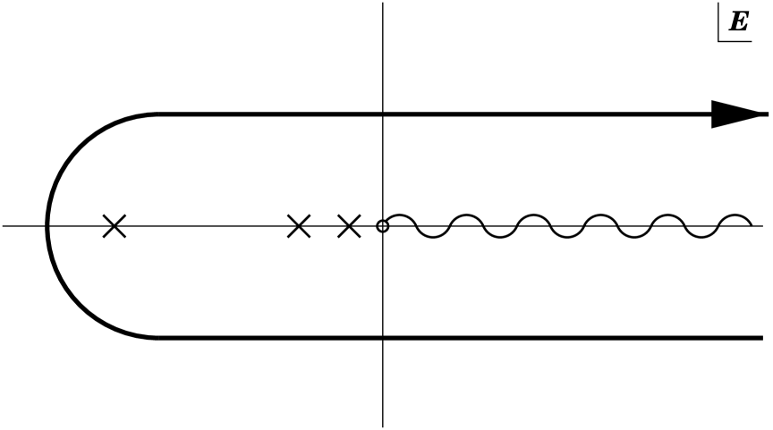
Figure 21: Integration contour for $F_{+}({\bf k})$. The Green’s function $G({\bf k},E)$ has a cut along the positive real axis and, in the case of an attractive potential, bound state poles at $E_{n}=-me^{4}/(2n^{2})$ for $n=1$, 2, … .

where the contour C, shown in Fig. 21, wraps clockwise about the cut along the positive real $E$ axis and also encircles all the bound-state poles which occur when $e^{2}<0$, corresponding to an attractive Coulomb potential. We shall first compute $G({\bf k},E)$ when the energy $E$ is real and sufficiently negative so that $E$ lies to the left of all singularities, and only later analytically continue to energies lying on the contour C. Thus at first we write

$$E=-{\gamma^{2}\over 2m}\,,$$ (D.10)

with $\gamma$ real and further restricted by $\gamma>|e^{2}|\,m$ when the potential is attractive. In view of the spherical symmetry of the problem, we may average over the orientations of ${\bf k}$ and use

$$G({\bf k},E)={\rm Tr}\,{1\over H-E}\,{\sin kr\over kr}\,.$$ (D.11)

In view of the cyclic symmetry of the trace, this may be expressed as

$$G({\bf k},E)={1\over k}\>{\rm Tr}\,{1\over\sqrt{r}(H-E)\sqrt{r}}\,\sin kr\,.$$ (D.12)

D.1 Coulomb $su(1,1)$ Symmetry

This latter form permits a remarkably simple evaluation by group theory. To do this, we first define the Hermitian operator

$${\cal J}_{0}={1\over 2\gamma}\,\sqrt{r}\,{\bf p}^{2}\sqrt{r}+{\gamma\over 2}\,r\,,$$ (D.13)

so that

$$\sqrt{r}\,(H-E)\sqrt{r}={\gamma\over m}\,{\cal J}_{0}+e^{2}\,.$$ (D.14)

The $\sqrt{r}$ transformation converts the energy eigenvalue problem to a coupling eigenvalue problem. To see this, we consider the Coulomb bound states $|nlm\rangle$ which have the fixed energy $-\gamma^{2}/2m$ that corresponds to (mutually attractive) charges $\pm e_{n}$ obeying the Bohr formula

$${\gamma^{2}\over 2m}={e_{n}^{4}\,m\over 2n^{2}}\,,$$ (D.15)

or

$$e_{n}^{2}=n\,{\gamma\over m}\,.$$ (D.16)

Hence,

$${\cal J}_{0}\,{1\over\sqrt{r}}\,|nlm\rangle = {m\over\gamma}\sqrt{r}\left[{{\bf p}^{2}\over 2m}+{\gamma^{2}\over 2m}\right]|nlm\rangle$$ (D.17)

$$= {m\over\gamma}\sqrt{r}\,{e_{n}^{2}\over r}\,|nlm\rangle$$

$$= n\,{1\over\sqrt{r}}\,|nlm\rangle\,,$$

and so the eigenvalues $j_{0}$ of ${\cal J}_{0}$ are the positive integers,

$$j_{0}=n\,,\qquad\qquad n=1,\,2,\,\ldots\,.$$ (D.18)

For a fixed principal quantum number $n$, $l$ ranges over $0\geq l\geq n-1$ and $m$ in turn varies through $-l\geq m\geq+l$. Thus the degeneracy of the $n$’th eigenvalue is

$$\sum_{l=0}^{n-1}\>(2l+1)=n^{2}\,.$$ (D.19)

To exploit the latent group properties, we introduce the Hermitian dilation operator which is conveniently labeled as

$${\cal J}_{2}={1\over 2}\left({\bf r}\cdot{\bf p}+{\bf p}\cdot{\bf r}\right),$$ (D.20)

and denote the commutator of ${\cal J}_{0}$ and ${\cal J}_{2}$ as ${\cal J}_{1}$ (times $-i$),

$$[{\cal J}_{0},{\cal J}_{2}]=-i{\cal J}_{1}\,.$$ (D.21)

Since

$$i\left[{\bf p},{\cal J}_{2}\right]={\bf p}\,,\qquad i\left[{\bf r},{\cal J}_{2}\right]=-{\bf r}\,,$$ (D.22)

${\cal J}_{1}$ differs from ${\cal J}_{0}$ merely by a sign change,

$${\cal J}_{1}={1\over 2\gamma}\,\sqrt{r}\,{\bf p}^{2}\sqrt{r}-{\gamma\over 2}\,r\,.$$ (D.23)

Moreover, a further commutation with ${\cal J}_{2}$ restores the original signs,

$$\left[{\cal J}_{1},{\cal J}_{2}\right]=-i{\cal J}_{0}\,.$$ (D.24)

And a straight forward computation of the final commutator shows that the algebra closes,

$$\left[{\cal J}_{0},{\cal J}_{1}\right]=i{\cal J}_{2}\,.$$ (D.25)

The three Pauli spin matrices $\sigma_{k}$ obey the $su(2)$ Lie algebra

$$\left[\sigma_{k},\sigma_{l}\right]=2i\,\epsilon_{klm}\,\sigma_{m}\,.$$ (D.26)

Thus, as far as the commutation relations go, we have the correspondences

$${\cal J}_{0}\leftrightarrow{1\over 2}\sigma_{3}\,,\quad{\cal J}_{1}\leftrightarrow{i\over 2}\sigma_{1}\,,\quad{\cal J}_{2}\leftrightarrow{i\over 2}\sigma_{2}\,,$$ (D.27)

which identifies the commutators of the ${\cal J}_{a}$ with the Lie algebra $su(1,1)$. This, of course, corresponds to a non-compact group which has infinite-dimensional irreducible representations.

With these results in hand, we return to our computation. Since

$${\cal J}_{0}-{\cal J}_{1}=\gamma\,r\,,$$ (D.28)

the sine function in Eq. (D.12) may be written in terms of group generators. Using this and the expression (D.14) for the denominator in Eq. (D.12), we obtain

$$G({\bf k},E)={m\over 2i\gamma k}\,{\rm Tr}\>{1\over{\cal J}_{0}+(me^{2}/\gamma)}\left[e^{ik({\cal J}_{0}-{\cal J}_{1})/\gamma}-e^{-ik({\cal J}_{0}-{\cal J}_{1})/\gamma}\right].$$ (D.29)

Representing the denominator in terms of the integral of an exponential now places the result in terms of the trace of the product of group elements:

$$G({\bf k},E)={m\over 2i\gamma k}\int_{0}^{\infty}ds\>e^{-(me^{2}/\gamma)s}\>{\rm Tr}\>e^{-s{\cal J}_{0}}\left[e^{ik({\cal J}_{0}-{\cal J}_{1})/\gamma}-e^{-ik({\cal J}_{0}-{\cal J}_{1})/\gamma}\right].$$ (D.30)

The products of two group elements may be expressed as a third group element. Since the trace is invariant under similarity transformations, this third group element may be “rotated” into one involving only the generator ${\cal J}_{0}$,

$${\rm Tr}\,e^{-s{\cal J}_{0}}e^{\pm ik({\cal J}_{0}-{\cal J}_{1})/\gamma}={\rm Tr}\,e^{-s_{\pm}{\cal J}_{0}}\,.$$ (D.31)

The required parameters $s_{\pm}$ will be determined momentarily. Evaluating the trace using the known eigenvalues $j_{0}{=}n$ of ${\cal J}_{0}$ with multiplicity $n^{2}$ yields

$${\rm Tr}\,e^{-s_{\pm}{\cal J}_{0}} = \sum_{n=1}^{\infty}n^{2}\,e^{-s_{\pm}n}=\left({\partial\over\partial s_{\pm}}\right)^{2}{1\over e^{s_{\pm}}-1}$$ (D.32)

$$= {1\over 4}\,{\cosh s_{\pm}/2\over\sinh^{3}s_{\pm}/2}\,.$$

Therefore

$$G({\bf k},E)={m\over 8i\gamma k}\int_{0}^{\infty}ds\,e^{-(me^{2}/\gamma)s}\left[{\cosh s_{+}/2\over\sinh^{3}s_{+}/2}-{\cosh s_{-}/2\over\sinh^{3}s_{-}/2}\right].$$ (D.33)

In view of the algebraic isomorphism between the group generators and the Pauli matrices, the parameters $s_{\pm}$ may be found by replacing the generators in Eq. (D.31) by the equivalent $2\times 2$ Pauli matrices. Hence,

$$2\cosh s_{\pm}/2 = {\rm tr}\exp\left\{-s_{\pm}{1\over 2}\sigma_{3}\right\}$$ (D.34)

$$= {\rm tr}\exp\left\{-s{1\over 2}\sigma_{3}\right\}\exp\left\{\pm{ik\over 2\gamma}(\sigma_{3}-i\sigma_{1})\right\}$$

$$= {\rm tr}\exp\left\{-s{1\over 2}\sigma_{3}\right\}\left[1\pm{ik\over 2\gamma}\left(\sigma_{3}-i\sigma_{1}\right)\right]$$

$$= e^{-s/2}\left[1\pm{ik\over 2\gamma}\right]+e^{+s/2}\left[1\mp{ik\over 2\gamma}\right].$$

We write

$$\left[1+{ik\over 2\gamma}\right]=e^{i\theta/2}\sqrt{1+{k^{2}\over 4\gamma^{2}}}$$ (D.35)

so that Eq. (D.34) becomes

$$\cosh s_{\pm}/2=\sqrt{1+{k^{2}\over 4\gamma^{2}}}\,\cosh(s\mp i\theta)/2\,.$$ (D.36)

A short calculation yields

$$\sinh^{2}s_{\pm}/2=\left(1+{k^{2}\over 4\gamma^{2}}\right)\,\left[\sinh^{2}(s\mp i\theta)/2+\sin^{2}\theta/2\right].$$ (D.37)

For later use, note that

$$\theta=2\arctan(k/2\gamma)=k/\gamma+O(k^{3})\,.$$ (D.38)

Hence

$$G({\bf k},E) = {m\over 8i\gamma k}{1\over 1+(k/2\gamma)^{2}}\int_{0}^{\infty}ds\>e^{-(me^{2}/\gamma)s}\left\{{\cosh(s-i\theta)/2\over[\sinh^{2}(s-i\theta)/2+\sin^{2}\theta/2]^{3/2}}\right.$$ (D.39)

$$\kern 166.2212pt\left.{}-{\cosh(s+i\theta)/2\over[\sinh^{2}(s+i\theta)/2+\sin^{2}\theta/2]^{3/2}}\right\}.$$

As noted in footnote 78, all along we should have subtracted the $e^{2}=0$ contribution from $G({\bf k},E)$. In the integral representation above, this simply means replacing $e^{-(me^{2}/\gamma)s}$ by the subtracted exponential $[e^{-(me^{2}/\gamma)s}-1]$. As anticipated, this subtraction removes what would otherwise be a singularity in the integral at $s=0$.

Figure 22: Integration contours for $G({\bf k},E)$.

D.2 Direct Contribution

To compute the integral (D.39) (with the $e^{2}{=}0$ piece removed), it is convenient to deform the path of integration into the contours shown in Fig. 22. For the first term in braces in the integrand, the contour is taken to run first over a portion of the imaginary axis, $s=i\phi,\,\,0<\phi<\theta$, and then to continue along the line parallel to the real axis, $s\to s+i\theta,\,\,0<s<\infty$. The integration contour for the second term in the braces is the complex conjugate of the first. These contour deformations produce

$$G({\bf k},E)={m\over 4\gamma k}\,{1\over 1+(k/2\gamma)^{2}}\left[J\!\left(\theta,{\textstyle{me^{2}\over\gamma}}\right)-\sin\!\left({\textstyle{me^{2}\over\gamma}}\,\theta\right)\,I\!\left(\theta,{\textstyle{me^{2}\over\gamma}}\right)\right],$$ (D.40)

where

$$J(\theta,z)=\int_{0}^{\theta}d\phi\,\left[\cos z\phi-1\right]{\cos(\theta-\phi)/2\over[\sin^{2}\theta/2-\sin^{2}(\theta-\phi)/2]^{3/2}}\,,$$ (D.41)

and

$$I(\theta,z)=\int_{0}^{\infty}ds\>e^{-zs}{\cosh s/2\over[\sinh^{2}s/2+\sin^{2}\theta/2]^{3/2}}\,.$$ (D.42)

Although this general result may be of interest in other contexts, here we are interested in the small $k^{2}$ behavior, since this determines the induced couplings in the effective theory. In the first integral $J(\theta,z)$, it is convenient to make the variable change $\phi=\theta(1{-}x)$ and write the integral as

$$J(\theta,z)=\theta\int_{0}^{1}dx\,\left[\cos z\theta(1{-}x)-1\right]{\cos\theta x/2\over[\sin^{2}\theta/2-\sin^{2}\theta x/2]^{3/2}}\,.$$ (D.43)

Recalling that $\theta\simeq k/\gamma$, we may expand the trigonometric functions in the integrand in Eq. (D.43) and keep only the leading terms to obtain

$$J(\theta,z)=-4z^{2}\int_{0}^{1}dx\>{(1-x)^{1/2}\over(1+x)^{3/2}}+O(\theta^{2})\,.$$ (D.44)

Writing $(1+x)^{-3/2}=-2(d/dx)(1+x)^{-1/2}$ and integrating by parts produces an end-point contribution and an integral made trivial by the substitution $x=\sin\chi$, and one finds that

$$J(\theta,z)=-z^{2}\>(8-2\pi)\;[1+O(\theta^{2})]\,.$$ (D.45)

If $I(\theta,z)$ is expanded in powers of $z$, the first three terms are singular as $\theta\to 0$, while all remaining terms have finite $\theta\to 0$ limits. It is convenient to separate the singular terms by writing

$$I(\theta,z)=I_{0}(\theta)-z\,I_{1}(\theta)+{\textstyle{1\over 2}}z^{2}\,I_{2}(\theta)+\bar{I}(\theta,z)\,,$$ (D.46)

where

$$I_{k}(\theta)\equiv\int_{0}^{\infty}ds\>{s^{k}\,\cosh s/2\over[\sinh^{2}s/2+\sin^{2}\theta/2]^{3/2}}\,,$$ (D.47)

and

$$\bar{I}(\theta,z)\equiv\int_{0}^{\infty}ds\,\left[e^{-zs}-1+zs-{\textstyle{1\over 2}}z^{2}s^{2}\right]{\cosh s/2\over[\sinh^{2}s/2+\sin^{2}\theta/2]^{3/2}}\,.$$ (D.48)

Since $d(\sinh s/2)=(ds/2)\cosh s/2$, the change of variable $\sinh s/2=\sin(\theta/2)\,\tan\chi$ makes the integral $I_{0}(\theta)$ elementary,

$$I_{0}(\theta)={2\over\sin^{2}\theta/2}\int_{0}^{\pi/2}d\chi\>\cos\chi={2\over\sin^{2}\theta/2}={8\over\theta^{2}}+{2\over 3}+O(\theta^{2})\,.$$ (D.49)

To evaluate $I_{1}(\theta)$ we write

$$I_{1}(\theta) = \int_{0}^{\infty}ds\>{8s\over[s^{2}+\theta^{2}]^{3/2}}+\int_{0}^{\infty}ds\>s\left({\cosh s/2\over[\sinh^{2}s/2+\sin^{2}\theta/2]^{3/2}}-{8\over[s^{2}+\theta^{2}]^{3/2}}\right).$$ (D.50)

The first integral, which is easy to evaluate, contains the piece which is singular as $\theta\to 0$, while the second integral is finite as $\theta\to 0$ and may be evaluated directly at $\theta=0$. Therefore,

$$I_{1}(\theta) = {8\over\theta}+\int_{0}^{\infty}ds\>\left(s\,{\cosh s/2\over\sinh^{3}s/2}-{8\over s^{2}}\right)+O(\theta)$$ (D.51)

$$= {8\over\theta}-\left.\left({s\over\sinh^{2}s/2}+2\,{\cosh s/2\over\sinh s/2}-{8\over s}\right)\right|_{0}^{\infty}+O(\theta)$$

$$= {8\over\theta}-2+O(\theta)\,.$$

A similar approach may be used for $I_{2}(\theta)$ if one first splits the integral into the contributions from $s<1$ and $s>1$,

$$I_{2}(\theta) = \int_{0}^{1}ds\>{8s^{2}\over[s^{2}+\theta^{2}]^{3/2}}+\int_{0}^{1}ds\>s^{2}\,\left({\cosh s/2\over[\sinh^{2}s/2+\sin^{2}\theta/2]^{3/2}}-{8\over[s^{2}+\theta^{2}]^{3/2}}\right)$$ (D.52)

$$\kern 86.72377pt{}+\int_{1}^{\infty}ds\>s^{2}\,{\cosh s/2\over[\sinh^{2}s/2+\sin^{2}\theta/2]^{3/2}}$$

$$= -8(1+\ln\theta/2)+\int_{0}^{1}ds\>\left(s^{2}{\cosh s/2\over\sinh^{3}s/2}-{8\over s}\right)+\int_{1}^{\infty}ds\>s^{2}\,{\cosh s/2\over\sinh^{3}s/2}+O(\theta)$$

$$= -8(1+\ln\theta/2)+\lim_{\epsilon\to 0}\left[8\ln\epsilon+\left.\left(8\ln\sinh s/2-{s^{2}\over\sinh^{2}s/2}-4s\,{\cosh s/2\over\sinh s/2}\right)\right|_{\epsilon}^{\infty}\right]+O(\theta)$$

$$= 4-8\ln\theta/2+O(\theta)\,.$$

The final integral $\bar{I}(\theta,z)$ is non-singular as $\theta\to 0$, and so we may simply set $\theta$ equal to zero and then integrate-by-parts twice,

$$\bar{I}(0,z) = -\int_{0}^{\infty}ds\,\left[e^{-zs}-1+zs-{\textstyle{1\over 2}}z^{2}s^{2}\right]{d\over ds}\,{1\over\sinh^{2}s/2}$$ (D.53)

$$= -z\int_{0}^{\infty}ds\,\left[e^{-zs}-1+zs\right]{1\over\sinh^{2}s/2}$$

$$= 4z\int_{0}^{\infty}ds\,\left[e^{-zs}-1+zs\right]{d\over ds}\,{1\over e^{s}-1}$$

$$= 4z^{2}\int_{0}^{\infty}ds\>{e^{-zs}-1\over e^{s}-1}\,.$$

The denominator may be expanded in a geometric series and the resulting $s$ integrals performed to give

$$\bar{I}(0,z)=-4z^{3}\sum_{l=1}^{\infty}{1\over l(l+z)}\,.$$ (D.54)

Using

$$\psi(z{+}1)+\gamma=z\sum_{l=1}^{\infty}{1\over l(l+z)}\,,$$ (D.55)

where $\psi(z)$ is the logarithmic derivative of the gamma function and $\gamma$ is Euler’s constant, yields the closed-form result

$$\bar{I}(0,z)=-4z^{2}\left[\psi(z{+}1)+\gamma\right].$$ (D.56)

This form may be used to make contact with the literature on quantum Coulomb corrections [4, 6]. A power series expansion in $z$ is obtained if the denominator in the sum (D.54) is expanded in powers of $z$ and the order of the resulting double sum interchanged. This process gives

$$\bar{I}(0,z)=4z^{2}\sum_{n=1}^{\infty}(-z)^{n}\zeta(n{+}1)\,,$$ (D.57)

where

$$\zeta(n)=\sum_{l=1}^{\infty}{1\over l^{n}}$$ (D.58)

is the Riemann $\zeta$ function.

Assembling the various pieces contributing to the Green’s function $G({\bf k},E)$ and inserting

$$\theta=(k/\gamma)-{\textstyle{1\over 12}}(k/\gamma)^{3}+O(k/\gamma)^{5}$$ (D.59)

produces

$$G({\bf k},E)=m\left\{-{2z\over k^{2}}+{\pi\over 2}{z^{2}\over\gamma k}+{1\over\gamma^{2}}\left[{z\over 6}-{z^{2}\over 2}-z^{3}\ln\biggl{(}{2\gamma\over k}\biggr{)}-{z^{3}\over 6}-{z\over 4}\,\bar{I}(0,z)\right]+O(k)\right\},$$ (D.60)

where $z=me^{2}/\gamma$. This result is to be inserted into the contour integral (D.9) relating $G({\bf k},E)$ to the thermal correlator $F_{+}({\bf k})$ which, with the $e^{2}=0$ subtraction made explicit, reads

$$\Delta F_{+}({\bf k})\equiv F_{+}({\bf k})-F_{+}^{0}({\bf k})=\int_{\rm C}{dE\over 2\pi i}\,e^{-\beta E}\,G({\bf k},E)\,.$$ (D.61)

Inserting the power series representation (D.57) for $\bar{I}(0,z)$ and recalling that $\gamma^{2}=-2mE$, the required contour integrals are easily performed using Hankel’s formula

$${1\over\Gamma(\alpha)}=\int_{C}{dt\over 2\pi i}\>(-t)^{-\alpha}\,e^{-t}\,,$$ (D.62)

and its derivative with respect to $\alpha$,

$${\psi(\alpha)\over\Gamma(\alpha)}=\int_{C}{dt\over 2\pi i}\>\ln(-t)\,(-t)^{-\alpha}\,e^{-t}\,.$$ (D.63)

The result, neglecting $O(k)$ contributions, is

$$\Delta F_{+}({\bf k}) = \biggl{(}{m\over 2\pi\beta}\biggr{)}^{3/2}\Bigg{\{}-{4\pi\beta e^{2}\over k^{2}}+{\pi^{2}\beta^{2}e^{4}\over k}$$ (D.64)

$$\quad\qquad\qquad{}+{\pi\beta^{3}e^{6}\over 3}\,\Biggl{[}\ln\biggl{(}{\beta k^{2}\over 2m}\biggr{)}+\gamma-3+{1\over\beta me^{4}}+f\Biggl{(}\sqrt{{\beta me^{4}\over 2\pi}}\Biggr{)}\Biggr{]}\Bigg{\}}\,,$$

where

$$f(y) \equiv -{3\over 4y}-{3\sqrt{\pi}\over 2}\sum_{n=1}^{\infty}\left(-\sqrt{\pi}\,y\right)^{n}{\zeta(n{+}1)\over\Gamma((n{+}5)/2)}\,.$$ (D.65)

Returning to our rationalized units with $e^{2}\to e_{a}e_{b}/4\pi$, replacing the mass parameter by the reduced mass, $m\to m_{ab}$, and writing the result in terms of the thermal wavelength corresponding to the reduced mass

$$\lambda_{ab}=\hbar\left({2\pi\beta\over m_{ab}}\right)^{1/2}$$ (D.66)

gives

$$\Delta F_{+}({\bf k}) = \lambda_{ab}^{-3}\>\Bigg{\{}-{\beta e_{a}e_{b}\over k^{2}}+{(\beta e_{a}e_{b})^{2}\over 16k}$$ (D.67)

$$\quad{}+\biggl{(}{\beta e_{a}e_{b}\over 4\pi}\biggr{)}^{3}\,{\pi\over 3}\left[\ln\biggl{(}{\lambda_{ab}^{2}k^{2}\over 4\pi}\biggr{)}+\gamma-3+{8\pi\lambda_{ab}^{2}\over(\beta e_{a}e_{b})^{2}}+f\biggl{(}{\beta e_{a}e_{b}\over 4\pi\lambda_{ab}}\biggr{)}\right]+O(k)\Bigg{\}}.$$

Evaluating $f(y)$ using the power series representation (D.65) is appropriate if $\beta e_{a}e_{b}/\lambda_{ab}$ is order one or smaller. But if $\beta e_{a}e_{b}/\lambda_{ab}$ is large, which corresponds to the formal $m\to\infty$ limit, one needs the asymptotic form of $f(y)$ for large argument. The result differs depending on whether the Coulomb interactions are attractive or repulsive. Consider the repulsive case first, where $z=me^{2}/\sqrt{-2mE}$ is positive on the negative real $E$ axis. In this case $\bar{I}(0,z)$ has no poles on the negative real $E$ axis, which reflects the absence of bound states for repulsive potentials. Thus, for repulsive interactions the contour integral (D.9) only wraps about the positive $E$ axis, and $\bar{I}(0,z)$ appears with $|\arg z|<\pi$. Hence the large $m$ limit may be obtained by using the large $z$ asymptotic behavior of the $\psi$ function,

$$\psi(z+1)\sim\ln z+{1\over 2z}-\sum_{n=1}^{\infty}{B_{2n}\over 2nz^{2n}}\,,\kern 75.88371pt\hbox{($|\arg z|<\pi$)}$$ (D.68)

where $B_{2n}$ are the Bernoulli numbers, to write the asymptotic form of Eq. (D.56) as

$$\bar{I}(0,z)\sim-4z^{2}\left(\ln z+\gamma+{1\over 2z}-\sum_{n=1}^{\infty}{B_{2n}\over 2nz^{2n}}\right).\qquad\hbox{($|\arg z|<\pi$)}$$ (D.69)

Using this form for $\bar{I}(0,z)$ and re-evaluating the contour integral (D.61) yields the asymptotic expansion for large positive argument,

$$f(y)\sim 2\,\ln(2\sqrt{\pi}y)+3\gamma-\frac{8}{3}-{3\over 2\sqrt{\pi}}\sum_{n=1}^{\infty}(-1)^{n}{B_{2n}\over 2n\pi^{n}y^{2n}}\,\Gamma(n{-}{\textstyle{3\over 2}})\,.$$ (D.70)

Evaluating the first term in the sum with $B_{2}=1/6$ and $\Gamma(-1/2)=-2\sqrt{\pi}$ yields

$$f(y)=2\,\ln(2\sqrt{\pi}y)+3\gamma-\frac{8}{3}-{1\over 4\pi y^{2}}+O(1/y^{4})\,.$$ (D.71)

To obtain the corresponding limit in the attractive case, note that Eq. (D.65) gives

$$f(y)-f(-y)=-{3\over 2y}+3\pi\sum_{m=0}^{\infty}\,{\zeta(2m+2)\over(m+2)!}\,\pi^{m}\,y^{2m+1}\,.$$ (D.72)

We insert the definition (D.58) of the $\zeta$ function and interchange the order of the summations. The sum over $m$ now produces an exponential with its first two expansion coefficients removed, and we obtain

$$f(y)-f(-y)=-{3\over 2y}+{3\over\pi\,y^{3}}\sum_{n=1}^{\infty}\,n^{2}\left[\,\exp\left\{{\pi\,y^{2}\over n^{2}}\right\}-1-{\pi\,y^{2}\over n^{2}}\right].$$ (D.73)

As $y\to-\infty$, the first term in the sum, which corresponds to the lowest bound state contribution, dominates,

$$f(y)\sim{3\over\pi\,y^{3}}\,\exp\left\{\pi\,y^{2}\right\}\,,$$ (D.74)

with exponentially small corrections.

D.3 Exchange Contribution

The same approach may be used to evaluate the exchange contribution

$$F_{-}({\bf k})={\rm Tr}\>{\cal P}\,e^{-\beta H}e^{-i{\bf k}\cdot{\bf r}}\,.$$ (D.75)

Since the parity operator $\cal P$ commutes with all the $su(1,1)$ group generators, all the previous formulas hold for this exchange term with the trivial change of an insertion of ${\cal P}$ in the trace defining the Green’s function. To evaluate the final trace

$${\rm Tr}\,{\cal P}\,e^{-s_{\pm}{\cal J}_{0}}\,,$$

we note that the $|nlm\rangle$ basis which diagonalizes ${\cal J}_{0}$ as shown in Eq. (D.17) has the familiar parity assignment of the hydrogen atom states,

$${\cal P}\,|nlm\rangle=|nlm\rangle\,(-1)^{l}\,.$$ (D.76)

Hence, we have essentially the same evaluation of the trace as before except that the previous degeneracy factor (D.19) is replaced by

$$\sum_{l=0}^{n-1}\,(-1)^{l}\,(2l+1)=-(-1)^{n}\,n\,.$$ (D.77)

Thus we now have

$${\rm Tr}\,{\cal P}\,e^{-s_{\pm}{\cal J}_{0}} = -\sum_{n=1}^{\infty}(-1)^{n}\,n\,e^{-s_{\pm}n}$$ (D.78)

$$= {1\over 4\cosh^{2}s_{\pm}/2}\,,$$

and Eq. (D.33) is replaced by

$$G_{-}({\bf k},E)={m\over 8i\gamma k}\int_{0}^{\infty}ds\,e^{-(me^{2}/\gamma)s}\left[{1\over\cosh^{2}s_{+}/2}-{1\over\cosh^{2}s_{-}/2}\right]\,.$$ (D.79)

We are interested in the (finite) ${\bf k}=0$ limit. Recalling Eq. (D.36) and that $\theta\sim k/\gamma$, this is given by

$$G_{-}({\bf 0},E) = {m\over 8\gamma^{2}}\int_{0}^{\infty}ds\>e^{-(me^{2}/\gamma)s}\,\lim_{\theta\to 0}\>{1\over i\theta}\left[{1\over\cosh^{2}(s-i\theta)/2}-{1\over\cosh^{2}(s+i\theta)/2}\right]\,,$$ (D.80)

$$= -{m\over 4\gamma^{2}}\int_{0}^{\infty}ds\,e^{-(me^{2}/\gamma)s}\,{d\over ds}\,{1\over\cosh^{2}s/2}\,.$$

Expressing the hyperbolic cosine in terms of exponentials and performing two partial integrations produces

$$G_{-}({\bf 0},E)={m\over\gamma^{2}}\>h\biggl{(}{me^{2}\over\gamma}\biggr{)}$$ (D.81)

with

$$h(z)={1\over 4}-{z\over 2}+z^{2}\int_{0}^{\infty}ds\>e^{-zs}\,{1\over e^{s}+1}\,.$$ (D.82)

Expanding the denominator and performing the $s$ integration gives

$$h(z)={1\over 4}-{z\over 2}+{z^{2}\over 2}\sum_{l=1}^{\infty}\left\{{1\over l+(z{-}1)/2}-{1\over l+z/2}\right\}\,.$$ (D.83)

Adding and subtracting $1/l$ in the sum, combining denominators, and referring to the representation (D.55), identifies the sum as the difference of two $\psi$ functions, and yields the closed form result

$$h(z)={1\over 4}-{z\over 2}+{z^{2}\over 2}\left[\psi\Biggl{(}{z{+}2\over 2}\Biggr{)}-\psi\Biggl{(}{z{+}1\over 2}\Biggr{)}\right].$$ (D.84)

Expanding the denominators in Eq. (D.83) in powers of $z$ and using

$$\sum_{l=1}^{\infty}\,{(-1)^{l+1}\over l^{z}}=\left[1-2^{1-z}\right]\zeta(z)$$ (D.85)

gives the useful power series expansion

$$h(z)={1\over 4}-{z\over 2}+z^{2}\,\sum_{n=0}^{\infty}\left(-z\right)^{n}(1-2^{-n})\,\zeta(n{+}1)\,.$$ (D.86)

Here the $n=0$ member of the sum is to be understood as containing

$$\lim_{z\to 1}\left[1-2^{1-z}\right]\zeta(z)=\sum_{l=1}^{\infty}\,{(-1)^{l+1}\over l}=\ln 2\,.$$ (D.87)

Inserting this series into the contour integral

$$F_{-}({\bf 0})=\int_{\rm C}{dE\over 2\pi i}\>e^{-\beta E}\,G_{-}({\bf 0},E)\,,$$ (D.88)

and again making use of Hankel’s formula (D.62) produces

$$F_{-}({\bf 0})=\biggl{(}{m\over 2\pi\beta}\biggr{)}^{3/2}\,\beta^{3}e^{6}\,{\pi\over 3}\,\tilde{f}\Biggl{(}\sqrt{{\beta me^{4}\over 2\pi}}\Biggr{)}\,,$$ (D.89)

where

$$\tilde{f}(y)={3\over 8\pi y^{3}}-{3\over 2\pi y^{2}}+{3\ln 2\over 2y}-{3\sqrt{\pi}\over 2}\sum_{n=0}^{\infty}\,\left(-\sqrt{\pi}\,y\right)^{n}\left[1-{1\over 2^{1+n}}\right]\,{\zeta(n{+}2)\over\Gamma((n{+}5)/2)}\,.$$ (D.90)

To obtain the behavior for the case of strong repulsion, that is, the large $y^{2}=\beta me^{4}/2$ limit, we return to the integral expression (D.82) for $h(z)$. Writing

$${1\over e^{s}+1}={1\over 2}-{1\over 2}\tanh{s\over 2}\,,$$ (D.91)

performing simple integrals, and rescaling the integration variable casts this integral representation in the form

$$h(z)=-{1\over 2}\int_{0}^{\infty}du\,e^{-u}\left[z\tanh\biggl{(}{u\over 2z}\biggr{)}-{u\over 2}\right].$$ (D.92)

This result shows explicitly that $h(z)$ is an even function of $z=me^{2}/\gamma$. Writing $E=p^{2}/2m$ sets $\gamma=\sqrt{-2mE}=ip$, with no problem with the sign of $i$ since only even functions of $\gamma$ appear. And, again because only even functions of $p$ appear, we may replace the contour integral (D.88) in the $E$ plane by a contour integral in the $p$ plane having the exactly the same contour. Thus

$$F_{-}({\bf 0})=-\int_{\rm C}{dp\over 2\pi i}\,{1\over p}\>e^{-\beta p^{2}/2m}\,h\!\left({me^{2}\over ip}\right).$$ (D.93)

Introducing the integral representation (D.92) into this contour integral, interchanging the integration order, and rescaling the contour integration variable by writing $p=2me^{2}\zeta/u$ yields

$$F_{-}({\bf 0})={1\over 4}\int_{0}^{\infty}du\,u\,e^{-u}\int_{\rm C}{d\zeta\over 2\pi i}\,{1\over\zeta}\>\exp\left\{-2\beta me^{4}\zeta^{2}/u^{2}\right\}\,\left[{\tan\zeta\over\zeta}-1\right].$$ (D.94)

The integrand of the contour integral has no pole at $\zeta=0$ since the quantity in the square brackets vanishes there. Thus the only singularities of the integrand come from the factor in square brackets, which has a series of simple poles at odd integer multiples of $\pi/2$ with residue $-1$. Since these poles are encircled in a negative, clockwise sense, we obtain

$$F_{-}({\bf 0})={1\over 4}\int_{0}^{\infty}du\,u\,e^{-u}\sum_{n=0}^{\infty}\left[{2\over(2n{+}1)\pi}\right]^{2}\>\exp\left\{-\beta me^{4}(2n{+}1)^{2}\pi^{2}/2u^{2}\right\}.$$ (D.95)

The leading asymptotic behavior is obtained by evaluating the $u$ integral, term-by-term, using the method of steepest descents. Only the $n=0$ term of the sum is relevant, since the remaining terms are exponentially smaller. Writing the result in terms of the function $\tilde{f}(y)$ defined in Eq. (D.89) with $y^{2}=\beta me^{4}/2\pi$ gives

$$\tilde{f}(y)\sim{3\over y^{3}\,\pi^{3}}\int_{0}^{\infty}du\,u\,e^{-u}\>\exp\left\{-y^{2}\pi^{3}/u^{2}\right\},$$ (D.96)

whose steepest descent evaluation yields

$$\tilde{f}(y)={2\sqrt{3}\over y^{2}\,\pi}\>\exp\left\{-{3\pi\over 2}\left(2y^{2}\right)^{1/3}\right\}\;\left[1+{17\over 18\pi}{1\over(2y^{2})^{1/3}}+\cdots\right]\,.$$ (D.97)

Since the exchange term involves interactions of a single particle type, the reduced mass $m$ appearing in the above formulae is $m_{a}/2$ for species $a$. Reverting to our rationalized units gives

$$F_{-}({\bf 0})=\lambda_{aa}^{-3}\,{3\over\pi}\,\biggl{(}{\beta e_{a}^{2}\over 4\pi}\biggr{)}^{3}\,\tilde{f}\biggl{(}{\beta e_{a}^{2}\over 4\pi\lambda_{aa}}\biggr{)}\,,$$ (D.98)

where $\lambda_{aa}=\sqrt{2}\lambda_{a}$. Note that here the argument of $\tilde{f}(y)$ is always positive.

Appendix E First Quantum Correction to Classical One-Component Plasma

Here we shall derive the leading, order $\hbar^{2}$, quantum correction to the $N$-particle canonical partition function of the classical, one-component plasma. This result appears in the literature [Eq. (24) of [5]], but we will give a self-contained pedagogical treatment. To do so, it is convenient first to examine the path integral representation of the single-particle partition function previously given in Eq. (B.21), namely

$$\int(d^{3}{\bf r})\>\langle{\bf r},\beta|{\bf r},0\rangle=\int[d{\bf r}]\>\exp\left\{-{1\over\hbar}\int_{0}^{\hbar\beta}d\tau\left[{m\over 2}\,{d{\bf r}\over d\tau}\cdot{d{\bf r}\over d\tau}+V({\bf r}(\tau))\right]\right\}\,.$$ (E.1)

We have explicitly displayed the factors of $\hbar$ which appear when $\beta$ and $\tau$ have their conventional units of inverse energy and time, respectively. We state again that the functional integral is over all paths which are periodic with period $\beta\hbar$. It is therefore convenient to use a Fourier series representation for the path, ${\bf r}(\tau)={\bf r}+{\bf\xi}(\tau)\,,$ in which

$${\bf\xi}(\tau)=\sum_{{n=-\infty\atop n\neq 0}}^{\infty}\,{\bf\xi}_{n}\,\exp\left\{-{2\pi i\,n\,\tau\over\hbar\beta}\right\}$$ (E.2)

contains the non-zero frequency fluctuations of the path about its mean position ${\bf r}$. As we shall see, the size of the fluctuations ${\bf\xi}(\tau)$ are of order $\hbar$. Since the (imaginary) time average of these fluctuations vanish, the leading quantum-mechanical correction appears in

$$\int(d^{3}{\bf r})\>\langle{\bf r},\beta|{\bf r},0\rangle = \int(d^{3}{\bf r})\>\exp\left\{-\beta V({\bf r})\right\}\int[d\xi]\exp\left\{-{\beta\,m\over 2}\sum_{{n=-\infty\atop n\neq 0}}^{\infty}\,\left({2\pi n\over\hbar\beta}\right)^{2}{\bf\xi}_{n}\cdot{\bf\xi}_{-n}\,\right\}$$ (E.3)

$$\kern 72.26999pt{}\times\left\{1-\beta\sum_{{n=-\infty\atop n\neq 0}}^{\infty}\,\xi^{k}_{n}\,\xi^{l}_{-n}\,\nabla_{k}\,\nabla_{l}\,V({\bf r})+O({\bf\xi}^{4})\right\}.$$

The path integral over the fluctuations defines a correlator which is just the inverse of the matrix defining the quadratic form in the exponential,

$$\langle\xi^{k}_{n}\,\xi^{l}_{-n^{\prime}}\rangle=\delta_{n,n^{\prime}}\,\delta^{kl}\,{1\over\beta m}\left({\hbar\beta\over 2\pi n}\right)^{2}\,.$$ (E.4)

Using

$$\sum_{{n=-\infty\atop n\neq 0}}^{\infty}{1\over 2n^{2}}=\zeta(2)={\pi^{2}\over 6}\,,$$ (E.5)

one immediately finds

$$\int(d^{3}{\bf r})\>\langle{\bf r},\beta|{\bf r},0\rangle=\langle{\bf r},\beta|{\bf r},0\rangle^{0}\int(d^{3}{\bf r})\>\exp\left\{-\beta V({\bf r})\right\}\left\{1-{\beta^{2}\hbar^{2}\over 24\,m}\,\nabla^{2}\,V({\bf r})+O(\hbar^{4})\right\}\,.$$ (E.6)

In other words, to $O(\hbar^{2})$, the effect of quantum fluctuations is equivalent to a shift in the potential energy $V({\bf r})$ appearing in the classical partition function by

$$\delta V({\bf r})={\beta\hbar^{2}\over 24\,m}\,\nabla^{2}\,V({\bf r})\,.$$ (E.7)

As a check on the result (E.6), we note that a partial integration of one of the gradients in the $\nabla^{2}$ term, together with the identification $\lambda^{2}=2\pi\hbar^{2}\beta/m$ and other minor notational changes, places this result in precisely the form of the first line of Eq. (B.54).

This result is easily extended to the case of the canonical partition function for $N$ particles. This case is represented by a path integral over the variables ${\bf r}_{a}(\tau)$, where $a=1,\,2,\,\cdots,\,N$,

$$Z_{N}=\int\prod_{a}[d{\bf r}_{a}]\>\exp\left\{-{1\over\hbar}\int_{0}^{\hbar\beta}d\tau\left[{m\over 2}\,\sum_{a}{d{\bf r}_{a}\over d\tau}\cdot{d{\bf r}_{a}\over d\tau}+{1\over 2}\sum_{a\neq b}V({\bf r}_{a}(\tau){-}{\bf r}_{b}(\tau))\right]\right\}\,.$$ (E.8)

The leading quantum, order $\hbar^{2}$, corrections come from the quadratic fluctuations in the coordinates ${\bf r}_{a}(\tau)$ and ${\bf r}_{b}(\tau)$ in each of the potential terms. Expanding these terms out from the exponential is performed in a compact fashion if the $N$-particle number densities are introduced,

$$n({\bf r})=\sum_{a=1}^{N}\,\delta({\bf r}{-}{\bf r}_{a})\,,$$ (E.9)

along with the canonical two-particle correlator

$$K_{N}({\bf r}-{\bf r}^{\prime})=\biggl{\langle}\sum_{a\neq b}\delta({\bf r}{-}{\bf r}_{a})\,\delta({\bf r}{-}{\bf r}_{b})\biggr{\rangle}=\Bigl{\langle}n({\bf r})\,n({\bf r}^{\prime})-\delta({\bf r}{-}{\bf r}^{\prime})\,n({\bf r})\Bigr{\rangle}\,.$$ (E.10)

With this notation, the change in the $N$-particle canonical partition function $Z_{N}$ for a general variation in the interparticle potential is given by

$$\delta\,\ln Z_{N}=-{\beta\over 2}\int(d^{3}{\bf r})(d^{3}{\bf r}^{\prime})\>K_{N}({\bf r}{-}{\bf r}^{\prime})\,\delta V({\bf r}{-}{\bf r}^{\prime})\,.$$ (E.11)

Thus, in view of the previous one-particle result (E.7), but keeping in mind that both the coordinates in the potential undergo fluctuations, we see that the leading quantum correction is given by

$$\delta\,\ln Z_{N}=-{\beta\over 2}\int(d^{3}{\bf r})(d^{3}{\bf r}^{\prime})\>K_{N}({\bf r}{-}{\bf r}^{\prime})\,{\beta\hbar^{2}\over 12m}\,\nabla^{2}\,V({\bf r}{-}{\bf r}^{\prime})\,.$$ (E.12)

Taking account of translational invariance, which gives an overall factor of the system volume ${\cal V}$, and remembering the definition $-\beta F=\ln Z_{N}$ of the Helmholtz free energy $F$, we have

$$\delta F={\beta\hbar^{2}\over 24\,m}\,{\cal V}\int(d^{3}{\bf r})\,K_{N}({\bf r})\,\nabla^{2}V({\bf r})\,.$$ (E.13)

This general result may be applied to a one-component plasma in the presence of a uniform neutralizing background charge density [since a strictly classical limit exists in this special case where the charge carriers all have a common sign of their charge]. However, one must be careful to properly handle the effect of the neutralizing background charge density before taking the thermodynamic limit. The easiest way to do so is to regard the interaction potential for the one-component plasma as the $\mu\to 0$ limit of the regularized potential

$$V({\bf r})=e^{2}\left({e^{-\mu r}\over 4\pi r}-{1\over{\cal V}\,\mu^{2}}\right).$$ (E.14)

The integral of this potential over the large volume ${\cal V}$ of the system vanishes, reflecting that a proper subtraction of the uniform background charge density has been performed. [Equivalently, this amounts to using a regularized Coulomb potential $e^{-\mu r}/(4\pi r)$ with a total charge density of $e[n({\bf r}){-}\bar{n}]$, where $\bar{n}=N/{\cal V}$ is the fixed average particle density.]

Now using

$$-\nabla^{2}V({\bf r})=e^{2}\left(\delta({\bf r})-\mu^{2}\,{e^{-\mu r}\over 4\pi r}\right),$$ (E.15)

Eq. (E.13) becomes

$$\delta\,F={\beta\hbar^{2}e^{2}\over 24\,m}\,{\cal V}\left[-K_{N}({\bf 0})+\lim_{\mu\to 0}\mu^{2}\int(d^{3}{\bf r})\>K_{N}({\bf r})\,{e^{-\mu r}\over 4\pi r}\right].$$ (E.16)

Because of the singularity of the Coulomb potential when $r\to 0$, the two-particle correlation $K_{N}({\bf r})$ vanishes as ${\bf r}\to 0$,

$$K_{N}({\bf r})\propto\exp\left\{-\beta V({\bf r})\right\}\to 0\;\hbox{as ${\bf r}\to 0$,}$$ (E.17)

and therefore the first term in Eq. (E.16) identically vanishes. On the other hand, at large separations, the number densities are not correlated, and so

$$K_{N}({\bf r})\to\left({N\over{\cal V}}\right)^{2}=\bar{n}^{2}\;\hbox{as ${\bf r}\to\infty$.}$$ (E.18)

For infinitesimal $\mu$, the integral in the second term of Eq. (E.16) is dominated by arbitrarily large distances, and hence one may simply replace $K_{N}({\bf r})$ in the integrand by its asymptotic value of $\bar{n}^{2}$. When multiplied by $\mu^{2}$, the resulting error one is making in the short distance part of the integral has no affect on the $\mu\to 0$ limit. Consequently,

$$\delta\,F = {\beta\hbar^{2}e^{2}\over 24\,m}\,{\cal V}\bar{n}^{2}\>\lim_{\mu\to 0}\>\mu^{2}\int(d^{3}{\bf r})\>{e^{-\mu r}\over 4\pi r}$$ (E.19)

$$= {\beta\hbar^{2}e^{2}\over 24\,m}\,{\cal V}\bar{n}^{2}\,.$$

Finally, the pressure is given by $p=-\partial F/\partial{\cal V}$ with $N$ and $\beta$ fixed. Thus, since ${\cal V}\bar{n}^{2}=N^{2}/{\cal V}$, we find that the first quantum correction to the pressure of classical one-component plasma is given by

$$\delta\left({\beta p\over n}\right)={\beta\hbar^{2}\over 24\,m}\,\beta e^{2}\,\bar{n}\,.$$ (E.20)

Recalling the definitions $\kappa^{2}=\beta e^{2}n$, $g=\beta e^{2}\kappa/4\pi$, $\lambda_{ee}^{2}=4\pi\beta\hbar^{2}/m$, and $\eta_{ee}=\beta e^{2}/(4\pi\lambda_{ee})$, we may rewrite this result as

$$\delta\left({\beta p\over n}\right)=g^{2}{\beta\hbar^{2}\over 24\,m}\left({4\pi\over\beta e^{2}}\right)^{2}={g^{2}\over 24}\left({1\over 4\pi\eta_{ee}^{2}}\right).$$ (E.21)

This correction agrees with that which appears in Eq. (5.33) in the text, as well as with the discussion of Eq. (24) in Ref. [5]. Note that since the $O(\hbar^{2})$ correction is proportional to $g^{2}$, it is entirely contained in the two-loop contribution of the equation of state; no $O(\hbar^{2})$ corrections are contained in any higher-loop contributions.

Appendix F Some Elements of Quantum Field Theory

Here we shall briefly derive and review some of the methods of quantum field theory that are used in the text. For simplicity we shall explicitly treat the case of the functional integral representation of the classical plasma without the induced interactions that provide the quantum corrections which make the theory finite. These additional interactions entail no essential changes in the techniques that we are about to outline, and their effects are easily described by including the appropriate additional terms in the functional integrand. In the same vein, we shall also neglect the quantum-mechanical imaginary time dependence discussed in Sec. 3.6. Thus we shall examine the generating functional

$$Z[\mu]={\rm Det}^{1/2}\left[-\beta\nabla^{2}\right]\int[d\phi]\exp\left\{-S[\phi;\mu]\right\},$$ (F.1)

in which

$$S[\phi;\mu]={\beta\over 2}\int(d^{\nu}{\bf r})\phi({\bf r})\left(-\nabla^{2}\right)\phi({\bf r})+S_{\rm int}[\phi;\mu]\,,$$ (F.2)

where

$$S_{\rm int}[\phi;\mu]=-{\sum}_{a}\int(d^{\nu}{\bf r})\,n^{0}_{a}({\bf r})\,e^{i\beta e_{a}\phi({\bf r})}\,.$$ (F.3)

With the generalized chemical potential functions $\mu_{a}({\bf r})$ taken to be constants, the generating functional $Z[\mu]$ reduces to the grand canonical partition function. Functional derivatives with respect to the generalized chemical potentials, with these potentials then taken to be constants, yield number density correlation functions.

F.1 Perturbation Theory

Perturbation theory developments of correlation functions can be done in essentially either of two ways: One can first perform the functional derivatives with respect to the generalized chemical potentials to bring down extra factors in the functional integrand that represent the particle densities and then set the chemical potentials to be constants and make a perturbative expansion. Or one can make a formal perturbative expansion of the functional integral with spatially varying, generalized chemical potentials $\mu_{a}({\bf r})$, and then expand the result in a spatial varying part of the chemical potentials to identify the correlation functions. Either case is subsumed in a slight generalization of the second way in which we write the functional integration field as $\phi({\bf r})=\bar{\phi}({\bf r})+\phi^{\prime}({\bf r})$, where $\bar{\phi}({\bf r})$ is some suitable background field. We then take out and explicitly display the pieces of zeroth and second order in the fluctuation field $\phi^{\prime}({\bf r})$. Since the background field $\bar{\phi}$ appears as a ‘constant’ translation in the (dummy) functional integration variable, $[d\phi]=[d\phi^{\prime}]$, and so with this separation and with an operator or infinite matrix notation,

$$Z[\mu] = {\rm Det}^{1/2}\left[-\beta\nabla^{2}\right]\,\exp\left\{-S[\bar{\phi};\mu]\right\}$$ (F.4)

$$\int[d\phi^{\prime}]\exp\left\{-(\beta/2)\phi^{\prime}\left[-\nabla^{2}+{\cal V}(\bar{\phi};\mu)\right]\phi^{\prime}\right\}F[\phi^{\prime}]\,.$$

Here

$${\cal V}(\bar{\phi};\mu;{\bf r})={\sum}_{a}\beta e_{a}^{2}\,n^{0}_{a}({\bf r})\,e^{i\beta e_{a}\bar{\phi}({\bf r})}\,,$$ (F.5)

and

$$F[\phi^{\prime}]=\exp\left\{-\tilde{S}_{\rm int}[\phi^{\prime};\bar{\phi},\mu]\right\}\cdots\,,$$ (F.6)

where $-\tilde{S}_{\rm int}[\phi^{\prime};\bar{\phi},\mu]$ contains the linear, cubic, and higher order terms in $\phi^{\prime}$ in the exponential. The ellipsis $\cdots$ stands for possible insertions in the integrand of the factors of the form $n^{0}_{a}e^{i\beta e_{a}\phi({\bf r})}$ that result in the first case above when functional derivative are first taken to construct correlation functions. We shall soon work out explicit examples that should make this perhaps somewhat abstract formulation clear.

To obtain the perturbative development, we first note that by completing the square to obtain a Gaussian functional integral which produces an infinite, Fredholm determinant, we have, using again an operator notation, the evaluation:

$$X[\zeta] = {\rm Det}^{1/2}\left[\beta(-\nabla^{2})\right]\int[d\phi^{\prime}]\exp\left\{-(\beta/2)\phi^{\prime}\left[-\nabla^{2}+{\cal V}(\bar{\phi};\mu)\right]\phi^{\prime}+i\phi^{\prime}\zeta\right\}$$ (F.7)

$$= {\rm Det}^{1/2}\left[\beta(-\nabla^{2})\right]{\rm Det}^{-1/2}\left[\beta(-\nabla^{2}+{\cal V})\right]\exp\left\{-(1/2\beta)\zeta G\zeta\right\}$$

$$= {\rm Det}^{-1/2}\left[1+{1\over-\nabla^{2}}{\cal V}\right]\exp\left\{-{1\over 2\beta}\int(d^{\nu}{\bf r})(d^{\nu}{\bf r}^{\prime})\zeta({\bf r})G({\bf r},{\bf r}^{\prime})\zeta({\bf r}^{\prime})\right\},$$

where in the last line we have noted that the product of determinants is the determinant of the product of operators and used ordinary notation with $G({\bf r},{\bf r}^{\prime})$ the Green’s function defined by

$$\left[-\nabla^{2}+{\cal V}(\bar{\phi};\mu;{\bf r})\right]G({\bf r},{\bf r}^{\prime})=\delta^{(\nu)}({\bf r}{-}{\bf r}^{\prime})\,.$$ (F.8)

We next note that

$$\exp\left\{-{1\over 2\beta}\int(d^{\nu}{\bf r})(d^{\nu}{\bf r}^{\prime})\zeta({\bf r})G({\bf r},{\bf r}^{\prime})\zeta({\bf r}^{\prime})\right\}=$$

$$\qquad\left.\exp\left\{{1\over 2\beta}\int(d^{\nu}{\bf r})(d^{\nu}{\bf r}^{\prime}){\delta\over\delta\phi({\bf r})}G({\bf r},{\bf r}^{\prime}){\delta\over\delta\phi({\bf r}^{\prime})}\right\}\exp\left\{i\int(d^{\nu}{\bf r})\phi({\bf r})\zeta({\bf r})\right\}\right|_{\phi=0}\,.$$ (F.9)

Hence the functional integral (F.7) defining $X[\zeta]$ may instead be replaced by an exponential functional derivative operation which, in the operator notation, reads

$$X[\zeta]={\rm Det}^{-1/2}\left[1+{1\over-\nabla^{2}}{\cal V}\right]\left.\exp\left\{{1\over 2\beta}{\delta\over\delta\phi^{\prime}}G{\delta\over\delta\phi^{\prime}}\right\}\exp\left\{i\phi^{\prime}\zeta\right\}\right|_{\phi^{\prime}=0}\,.$$ (F.10)

Now the functional $X[\zeta]$ defined by the functional integral (F.7) has precisely the same form as the functional integral (F.4) defining the thermodynamic generating functional $Z[\mu]$ except that $F[\phi^{\prime}]$ is replaced by the functional Fourier transform factor $\exp\{i\phi^{\prime}\zeta\}$. Since this functional Fourier transform factor can be used to generate any functional, we conclude that

$$Z[\mu] = {\rm Det}^{-1/2}\left[1+{1\over-\nabla^{2}}{\cal V}\right]\exp\left\{-S[\bar{\phi};\mu]\right\}$$ (F.11)

$$\left.\exp\left\{{1\over 2\beta}\int(d^{\nu}{\bf r})(d^{\nu}{\bf r}^{\prime}){\delta\over\delta\phi^{\prime}({\bf r})}G({\bf r},{\bf r}^{\prime}){\delta\over\delta\phi^{\prime}({\bf r}^{\prime})}\right\}F[\phi^{\prime}]\right|_{\phi^{\prime}=0}\,.$$

This is the functional form than lends itself to a perturbative development by expanding the exponential of the functional derivatives. Performing the functional derivatives produces the “Wick contractions” that are familiar in quantum field theory and lead to the familiar graphical representation. The exact analytic form with the proper numerical factors associated with a given graph is easily obtained from the expansion of the exponential and the operation of the functional derivatives.

F.2 Straightforward Expansions

We consider the ordinary partition function in which all the chemical potentials are constants. This will illustrate the use of this functional derivative formulation in a straightforward fashion. In this case we take the background field to vanish, $\bar{\phi}=0$, and so the quadratic part of the action involves the lowest-order Debye (squared) wave number

$$\kappa_{0}^{2}=\beta\sum_{a=1}^{A}e_{a}^{2}n^{0}_{a}\,,$$ (F.12)

with ${\cal V}\to\kappa_{0}^{2}$, and so the Green’s function reduces to the Debye Green’s function $G_{\nu}({\bf r}{-}{\bf r}^{\prime})$ that was defined previously in Eq. (2.57). With constant chemical potentials and with $\bar{\phi}=0$,

$$-S[0;\mu]={\sum}_{a}n^{0}_{a}\int(d^{\nu}{\bf r})\,,$$ (F.13)

while the determinantal prefactor reduces to that evaluated previously in Eq. (2.77) of the text,

$${\rm Det}^{-1/2}\left[1+{1\over-\nabla^{2}}\kappa_{0}^{2}\right]=\exp\left\{-G_{\nu}({\bf 0}){1\over\nu}\kappa_{0}^{2}\int(d^{\nu}{\bf r})\right\}.$$ (F.14)

Therefore, the first two factors in the general perturbative formula (F.11) yield the partition function valid up to one-loop order,

$$Z_{1}=\exp\left\{\left[\sum n^{0}_{a}-G_{\nu}({\bf 0}){\kappa_{0}^{2}\over\nu}\right]\int(d^{\nu}{\bf r})\right\},$$ (F.15)

the result (2.78) in the text, and hence

$$Z[\mu]=Z_{1}\left.\exp\left\{{1\over 2\beta}\int(d^{\nu}{\bf r})(d^{\nu}{\bf r}^{\prime}){\delta\over\delta\phi({\bf r})}G_{\nu}({\bf r}{-}{\bf r}^{\prime}){\delta\over\delta\phi({\bf r}^{\prime})}\right\}\exp\left\{-\tilde{S}_{\rm int}[\phi;\mu]\right\}\right|_{\phi=0}\,.$$ (F.16)

Here

$$-\tilde{S}_{\rm int}[\phi;\mu]=\int(d^{\nu}{\bf r}){\sum}_{a}\,n^{0}_{a}\left\{e^{i\beta e_{a}\phi({\bf r})}-1+{1\over 2}\left[\beta e_{a}\phi({\bf r})\right]^{2}\right\}.$$ (F.17)

As a first application of of this method, we derive the result (2.64) for $\left<\!\left<\phi\right>\!\right>^{(1)}$ given in the text. To all orders

$$\left<\!\left<\phi({\bf 0})\right>\!\right> = Z[\mu]^{-1}Z_{1}\exp\left\{{1\over 2\beta}\int(d^{\nu}{\bf r}_{1})(d^{\nu}{\bf r}_{2}){\delta\over\delta\phi({\bf r}_{1})}G_{\nu}({\bf r}_{1}-{\bf r}_{2}){\delta\over\delta\phi({\bf r}_{2})}\right\}$$ (F.18)

$$\qquad\left.\Bigg{\{}\phi({\bf 0})\exp\left\{-\tilde{S}_{\rm int}[\phi;\mu]\right\}\Bigg{\}}\right|_{\phi=0}\,.$$

To the desired one-loop order, with the linear coupling to $\phi$ counted as itself of one-loop order as explained in the discussion of Eq. (2.64) of the text,

$$\left<\!\left<\phi({\bf 0})\right>\!\right>^{(1)} = \exp\left\{{1\over 2\beta}\int(d^{\nu}{\bf r}_{1})(d^{\nu}{\bf r}_{2}){\delta\over\delta\phi({\bf r}_{1})}G_{\nu}({\bf r}_{1}-{\bf r}_{2}){\delta\over\delta\phi({\bf r}_{2})}\right\}$$ (F.19)

$$\qquad\qquad\left.\Bigg{\{}\phi({\bf 0})\sum_{a=1}^{A}n^{0}_{a}\int(d^{\nu}{\bf r})\left[(i\beta e_{a}\phi({\bf r}))+{\textstyle{1\over 3!}}(i\beta e_{a}\phi({\bf r}))^{3}\right]\Bigg{\}}\right|_{\phi=0}$$

$$= \left\{{1\over 2\beta}\int(d^{\nu}{\bf r}_{1})(d^{\nu}{\bf r}_{2}){\delta\over\delta\phi({\bf r}_{1})}G_{\nu}({\bf r}_{1}-{\bf r}_{2}){\delta\over\delta\phi({\bf r}_{2})}\right\}$$

$$\qquad\qquad\phi({\bf 0})\sum_{a=1}^{A}n^{0}_{a}\int(d^{\nu}{\bf r})(i\beta e_{a}\phi({\bf r}))$$

$$+{1\over 2}\left\{{1\over 2\beta}\int(d^{\nu}{\bf r}_{1})(d^{\nu}{\bf r}_{2}){\delta\over\delta\phi({\bf r}_{1})}G_{\nu}({\bf r}_{1}-{\bf r}_{2}){\delta\over\delta\phi({\bf r}_{2})}\right\}^{2}$$

$$\qquad\qquad\phi({\bf 0})\sum_{a=1}^{A}n^{0}_{a}\int(d^{\nu}{\bf r}){\textstyle{1\over 3!}}(i\beta e_{a}\phi({\bf r}))^{3}$$

$$= i\int(d^{\nu}{\bf r})G_{\nu}({\bf 0}-{\bf r})\sum_{a=1}^{A}e_{a}n^{0}_{a}\left[1-{1\over 2}\beta e_{a}^{2}G_{\nu}({\bf 0})\right].$$

In view of the Fourier representation (2.57) of the Debye Green’s function,

$$\int(d^{\nu}{\bf r})G_{\nu}({\bf 0}-{\bf r})={1\over\kappa_{0}^{2}}\,,$$ (F.20)

and so

$$\left<\!\left<\phi\right>\!\right>^{(1)}={i\over\kappa_{0}^{2}}\sum_{a=1}^{A}e_{a}n^{0}_{a}\left[1-{1\over 2}\beta e_{a}^{2}G_{\nu}({\bf 0})\right],$$ (F.21)

which is just the result (2.64) of the text.

The perturbative expansions of the density and density–density correlations discussed in the text follow from

$$\left<\!\left<n_{a}({\bf r})\right>\!\right> = Z[\mu]^{-1}Z_{1}\exp\left\{{1\over 2\beta}\int(d^{\nu}{\bf r}_{1})(d^{\nu}{\bf r}_{2}){\delta\over\delta\phi({\bf r}_{1})}G_{\nu}({\bf r}_{1}-{\bf r}_{2}){\delta\over\delta\phi({\bf r}_{2})}\right\}$$ (F.22)

$$\qquad\left.\Bigg{\{}n^{0}_{a}\,e^{i\beta e_{a}\phi({\bf r})}\,\exp\left\{-\tilde{S}_{\rm int}[\phi;\mu]\right\}\Bigg{\}}\right|_{\phi=0}\,,$$

and

$$\left<\!\left<n_{a}({\bf r})n_{b}({\bf r}^{\prime})\right>\!\right> = Z[\mu]^{-1}Z_{1}\exp\left\{{1\over 2\beta}\int(d^{\nu}{\bf r}_{1})(d^{\nu}{\bf r}_{2}){\delta\over\delta\phi({\bf r}_{1})}G_{\nu}({\bf r}_{1}-{\bf r}_{2}){\delta\over\delta\phi({\bf r}_{2})}\right\}$$ (F.23)

$$\quad\left.\Bigg{\{}n^{0}_{a}\,e^{i\beta e_{a}\phi({\bf r})}n^{0}_{b}\,\,e^{i\beta e_{b}\phi({\bf r}^{\prime})}\,\exp\left\{-\tilde{S}_{\rm int}[\phi;\mu]\right\}\Bigg{\}}\right|_{\phi=0}\,.$$

F.3 Loop Parameter

It was emphasized in the text that the size of loop corrections is measured, in $\nu$ dimensions, by the dimensionless parameter $\beta e^{2}G_{\nu}({\bf 0})\sim\beta e^{2}\kappa_{0}^{\nu-2}$, which reduces to $\beta e^{2}\kappa_{0}$ in three dimensions: A perturbative term corresponding to a graph containing $\ell$ loops is of order $[\beta e^{2}\kappa_{0}^{\nu-2}]^{\ell}$ , or in three dimensions, $[\beta e^{2}\kappa_{0}]^{\ell}$. That is, the power of $[\beta e^{2}\kappa_{0}]$ counts the loop order of the expression. It should be noted that these loop graphs are connected and single-particle irreducible. In this counting, $e^{2}$ denotes a generic, typical charge of any of the particle species, or, equivalently, one could write $e_{a}=Z_{a}e$, and $e$ is the electron charge. Here we shall sketch the proof of this assertion.

To do this, we examine the expansion of the perturbative formula (F.16) in powers of the unperturbed densities, which we write in the schematic form

$$Z_{N}[\mu] \sim {1\over N!}\exp\left\{{1\over 2\beta}\int(d^{\nu}{\bf r})(d^{\nu}{\bf r}^{\prime}){\delta\over\delta\phi({\bf r})}G_{\nu}({\bf r}{-}{\bf r}^{\prime}){\delta\over\delta\phi({\bf r}^{\prime})}\right\}$$

$$\left.\int(d^{\nu}{\bf r}_{1})\,n^{0}({\bf r})e^{i\beta e\phi({\bf r}_{1})}\int(d^{\nu}{\bf r}_{2})\,n^{0}({\bf r})e^{i\beta e\phi({\bf r}_{2})}\cdots\int(d^{\nu}{\bf r}_{N})\,n^{0}({\bf r})e^{i\beta e\phi({\bf r}_{N})}\right|_{\phi=0}\,.$$

This corresponds to a graph with $N$ vertices. Functional derivatives with respect to $\mu({\bf r})$ may be taken to give number density correlators. We have omitted the subtraction of the unit and $\phi^{2}$ terms which appear in the interaction part of the action (F.17), which we may do with the understanding that at least three $\phi$ functional derivatives are taken at each vertex or that each vertex emits at least three propagator lines.

Let us first assume that functional derivatives have been taken so that each vertex is connected by a single propagator line. At this stage, we have a graph which is a polygon with $N$ lines and $N$ vertices. Note that since our counting applies to connected, single-particle irreducible graphs, any of these graphs must have such a perimeter polygon. To exhibit the parameters, we introduce dimensionless spatial coordinates by writing ${\bf r}={\bf q}/\kappa_{0}$. Then the propagator $G_{\nu}({\bf r}{-}{\bf r}^{\prime})$ becomes $\kappa_{0}^{\nu-2}$ times a dimensionless function of the dimensionless variable $({\bf q}-{\bf q}^{\prime})$. The functional derivative operations in Eq. (LABEL:schem) produce a propagator line times $\beta^{-1}$ with a factor of $\beta e$ at each end of the line. Thus for each propagator line and the vertex factors associated with both ends of the line we have an overall factor of $\beta e^{2}\kappa_{0}^{\nu-2}$. Each vertex involves $\int(d^{\nu}{\bf r})\sim\kappa_{0}^{-\nu}$ times $n^{0}$ (a dimensionless product), and so, all together for our skeleton polygon, we have $N$ factors of $\beta e^{2}n^{0}\kappa_{0}^{-2}$. But $\beta e^{2}n^{0}\sim\kappa_{0}^{2}$, and so these are just $N$ factors of $1$. If we measure the size of this skeleton one-loop graph in term of the unperturbed grand potential $\beta\Omega\sim\int(d^{\nu}{\bf r})n^{0}$, then one factor of $\beta e^{2}\kappa_{0}^{\nu-2}$ remains to characterize the order of the one-loop graph.

The remainder of the proof is now trivial. Each additional propagator line added to the skeleton polygon gives a factor $\beta e^{2}\kappa_{0}^{\nu-2}$ and increases the number of loops by one.

Appendix G Calculations Using Functional Methods

We turn now to apply the functional methods using the alternative background field method mentioned in the preceding Appendix. We choose the background field $\bar{\phi}({\bf r})$ used there to be the solution $\phi_{\rm cl}({\bf r})$ of the classical field equation of the total action which now contains a source:

$$S_{\rm tot}[\phi;\sigma;\mu] = S[\phi;\mu]-\beta\int(d^{\nu}{\bf r})\phi({\bf r})\sigma({\bf r})$$ (G.1)

$$= \int(d^{\nu}{\bf r})\left\{{\beta\over 2}\phi\left(-\nabla^{2}\right)\phi-{\sum}_{a}n_{a}({\bf r})\exp\{i\beta e_{a}\phi\}-\beta\phi\sigma\right\}.$$

Thus $\phi_{\rm cl}({\bf r})$ is defined by

$$-\nabla^{2}\phi_{\rm cl}({\bf r})=i\,{\sum}_{a}e_{a}n_{a}^{0}({\bf r})\exp\{i\beta e_{a}\phi({\bf r})\}+\sigma({\bf r})\,.$$ (G.2)

This choice is made because, since the action is stationary for variations about the solution of the classical field equation, with $\phi=\phi_{\rm cl}+\phi^{\prime}$, there are no linear terms in the fluctuation field $\phi^{\prime}$ and the result (F.11) of the previous Appendix takes the form

$$\exp\{W[\sigma;\mu]\} = {\rm Det}^{-1/2}\left[1+{1\over-\nabla^{2}}{\cal V}[\phi_{\rm cl};\mu]\right]\exp\left\{-S_{\rm tot}[\phi_{\rm cl};\sigma;\mu]\right\}$$

$$\left.\exp\left\{{1\over 2\beta}\int(d^{\nu}{\bf r})(d^{\nu}{\bf r}^{\prime}){\delta\over\delta\phi^{\prime}({\bf r})}G({\bf r},{\bf r}^{\prime}){\delta\over\delta\phi^{\prime}({\bf r}^{\prime})}\right\}\exp\{-\tilde{S}_{\rm int}[\phi^{\prime};\phi_{\rm cl},\mu]\}\right|_{\phi^{\prime}=0}\,.$$

Here

$${\cal V}(\phi_{\rm cl};\mu;{\bf r})={\sum}_{a}\beta e_{a}^{2}\,n^{0}_{a}({\bf r})\,e^{i\beta e_{a}\phi_{\rm cl}({\bf r})}\,,$$ (G.4)

with

$$\left\{-\nabla^{2}+{\cal V}(\phi_{\rm cl};\mu;{\bf r})\right\}G({\bf r},{\bf r}^{\prime})=\delta({\bf r}{-}{\bf r}^{\prime})\,,$$ (G.5)

and

$$-\tilde{S}_{\rm int}[\phi^{\prime};\phi_{\rm cl},\mu] = \int(d^{\nu}{\bf r}){\sum}_{a}\,n^{0}_{a}({\bf r})\,e^{i\beta e_{a}\phi_{\rm cl}({\bf r})}\left\{e^{i\beta e_{a}\phi^{\prime}({\bf r})}-1-i\beta e_{a}\phi^{\prime}({\bf r})+{1\over 2}\left[\beta e_{a}\phi^{\prime}({\bf r})\right]^{2}\right\}\,.$$

G.1 Results Through One Loop

We shall make use of this general result in the next section where the two-loop correction will be evaluated. Here we note that action of the exponential of functional derivatives on the exponential of $\tilde{S}_{\rm int}$ produces only two and higher order loops since $\tilde{S}_{\rm int}$ contains no linear terms in $\phi^{\prime}$. Hence, to the one-loop order with which we are concerned here, we have

$$W[\sigma;\mu]=W^{(1)}[\sigma;\mu]=-S_{\rm tot}[\phi_{\rm cl};\sigma;\mu]-{1\over 2}\ln{\rm Det}\left[1+{1\over-\nabla^{2}}{\cal V}[\phi_{\rm cl};\mu]\right].$$ (G.7)

To obtain the effective action described in Appendix A, we first need the relation between

$$\langle\phi({\bf r})\rangle_{\beta}^{\sigma}={\delta W[\sigma;\mu]\over\delta\beta\sigma({\bf r})}$$ (G.8)

and $\phi_{\rm cl}({\bf r})$. Since the action $S_{\rm tot}[\phi_{\rm cl};\sigma;\mu]$ is stationary for field variations about $\phi_{\rm cl}$, the induced variation in $\phi_{\rm cl}$ when the source $\sigma$ is varied does not contribute to $\delta S_{\rm tot}$ and only the explicit source variation contributes, giving

$$-{\delta S_{\rm tot}[\phi_{\rm cl};\sigma;\mu]\over\delta\beta\sigma({\bf r})}=\phi_{\rm cl}({\bf r})\,.$$ (G.9)

This is the classical or tree contribution. Using the formula $\delta\ln{\rm Det}X={\rm Tr}X^{-1}\delta X$, the one loop contribution is contained in

$$\delta\ln{\rm Det}\left[1+{1\over-\nabla^{2}}{\cal V}[\phi_{\rm cl};\mu]\right] = {\rm Tr}\left[1+{1\over-\nabla^{2}}{\cal V}[\phi_{\rm cl};\mu]\right]^{-1}{1\over-\nabla^{2}}\delta{\cal V}[\phi_{\rm cl};\mu]$$ (G.10)

$$= {\rm Tr}\left[-\nabla^{2}+{\cal V}[\phi_{\rm cl};\mu]\right]^{-1}\delta{\cal V}[\phi_{\rm cl};\mu]$$

$$= \int(d^{\nu}{\bf r})G({\bf r},{\bf r})i\beta g_{3}({\bf r})\,\delta\phi_{\rm cl}({\bf r})\,,$$

where

$$g_{3}({\bf r})={\sum}_{a}\beta e_{a}^{3}\,n^{0}_{a}({\bf r})\,e^{i\beta e_{a}\phi_{\rm cl}({\bf r})}\,.$$ (G.11)

The variation of the equation (G.2) defining the classical solution yields

$$\left\{-\nabla^{2}+{\cal V}(\phi_{\rm cl};\mu;{\bf r})\right\}\delta\phi_{\rm cl}({\bf r})=\delta\sigma({\bf r})\,,$$ (G.12)

and so

$${\delta\phi_{\rm cl}({\bf r})\over\delta\sigma({\bf r}^{\prime})}=G({\bf r},{\bf r}^{\prime})\,.$$ (G.13)

Hence, to one-loop order,

$$\langle\phi({\bf r})\rangle^{(1)}={\delta W^{(1)}[\sigma;\mu]\over\delta\beta\sigma({\bf r})}=\phi_{\rm cl}({\bf r})+\Delta\phi({\bf r})\,,$$ (G.14)

where

$$\Delta\phi({\bf r})=-{i\over 2}\int(d^{\nu}{\bf r}^{\prime})G({\bf r},{\bf r}^{\prime})g_{3}({\bf r}^{\prime})G({\bf r}^{\prime},{\bf r}^{\prime})\,.$$ (G.15)

The correction $\Delta\phi({\bf r})$ is a one-loop contribution corresponding to a “tadpole” graph. This graph is just the same as the second graph in Fig. 11 except that now the vertex is given by $g_{3}({\bf r}^{\prime})$ and the lines represent the Green’s function $G({\bf r},{\bf r}^{\prime})$. With the source vanishing, and with $\sum e_{a}n_{a}^{0}$ taken to be of one-loop order, $\phi_{\rm cl}=(i/\kappa_{0}^{2})\sum e_{a}n_{a}^{0}$ to this order. Thus, to one-loop order, $\phi_{\rm cl}$ can be taken to vanish in the explicitly one-loop term $\Delta\phi$, and the Green’s functions there can be replaced by the Debye functions. With these remarks in mind, it is easy to check that general one-loop result (G.14) reduces to the previous result (F.21).

The effective potential is taken to be a functional of the field expectation value which we relabel as $\bar{\phi}({\bf r})$. The one-loop action (G.7) is a functional of the classical field $\phi_{\rm cl}({\bf r})$ which differs from the expectation value by the one-loop correction $\Delta\phi({\bf r})$. Since the classical action is stationary for variations about $\phi_{\rm cl}({\bf r})$, replacing $\phi_{\rm cl}({\bf r})$ in it by $\bar{\phi}({\bf r})$ entails a correction involving $\Delta\phi({\bf r})^{2}$, which is of two-loop order. Since the determinantal contribution is already of first order, replacing $\phi_{\rm cl}({\bf r})$ in it by $\bar{\phi}({\bf r})$ also gives a two-loop correction. Thus, to one-loop order, we may replace $\phi_{\rm cl}({\bf r})$ by $\bar{\phi}({\bf r})$ in the action functional (G.7). [The explicit form for $\Delta\phi$ given in the previous paragraph is, of course, not needed to reach this conclusion. We made this explicit calculation because the result will be used in the next section on the two-loop effective action.] The effective action for the time-independent field $\bar{\phi}$ is defined by simply restricting the Legendre transformation (A.21) to involve time-independent quantities so that the imaginary time integral is replaced by a factor of $\beta$. The source–field product in the Legendre transformation cancels the source term in the relation (G.1) between $S_{\rm tot}[\phi;\sigma\mu]$ and $S[\phi;\mu]$, and we have to one-loop order

$$\Gamma^{(1)}[\bar{\phi};\mu]=S[\bar{\phi};\mu]+{1\over 2}\ln{\rm Det}\left[1+{1\over-\nabla^{2}}{\cal V}[\bar{\phi};\mu]\right].$$ (G.16)

It proves convenient to rewrite the determinant in the form:

$${\rm Det}\left[1+{1\over-\nabla^{2}}{\cal V}\right] = {\rm Det}\left[{1\over-\nabla^{2}}\left\{-\nabla^{2}+\kappa_{0}^{2}+\left({\cal V}-\kappa_{0}^{2}\right)\right\}\right]$$ (G.17)

$$= {\rm Det}\left[1+{1\over-\nabla^{2}}\kappa_{0}^{2}\right]{\rm Det}\left[1+G_{\nu}\left({\cal V}-\kappa_{0}^{2}\right)\right]\,.$$

Here we have added and subtracted the (squared) Debye wave number $\kappa_{0}^{2}$ for the (lowest-order) densities when the generalized chemical potentials reduce to the their standard, spatially uniform form, $\mu_{a}({\bf r})\to\mu_{a}$, and $G_{\nu}$ is the Debye Green’s function for this wave number. The first factor in Eq. (G.17) is the one-loop correction to the standard partition function; in the limit in which the generalized chemical potentials become constant and $\bar{\phi}=0$, ${\cal V}=0$, and we see that since

$$\left.S[\bar{\phi};\mu]\right|_{0}=-\int(d^{\nu}{\bf r})n^{0}_{a}\,,$$ (G.18)

the grand partition function to one-loop order is given by

$$\ln Z_{1} = -\left.\Gamma^{(1)}[\bar{\phi};\mu]\right|_{0}$$ (G.19)

$$= n^{0}_{a}{\cal V}-{1\over 2}\ln{\rm Det}\left[1+{1\over-\nabla^{2}}\kappa_{0}^{2}\right],$$

in agreement with Eq. (2.54).

To compute the number densities and number-density correlation functions to one-loop order, we first note that

$$\ln{\rm Det}\left[1+G_{\nu}\left({\cal V}-\kappa_{0}^{2}\right)\right] = {\rm Tr}\ln\left[1+G_{\nu}\left({\cal V}-\kappa_{0}^{2}\right)\right]$$

$$= {\rm Tr}G_{\nu}\,\left({\cal V}-\kappa_{0}^{2}\right)-{1\over 2}{\rm Tr}\left[G_{\nu}\left({\cal V}-\kappa_{0}^{2}\right)\right]^{2}+\cdots$$

$$= G_{\nu}({\bf 0})\int(d^{\nu}{\bf r}_{1})\left({\cal V}(\bar{\phi};\mu;{\bf r}_{1})-\kappa_{0}^{2}\right)$$

$$-{1\over 2}\int(d^{\nu}{\bf r}_{1})(d^{\nu}{\bf r}_{2})\!\!\! \!\!\!\left[G_{\nu}({\bf r}_{1}-{\bf r}_{2})\right]^{2}\left({\cal V}(\bar{\phi};\mu;{\bf r}_{1})-\kappa_{0}^{2}\right)\left({\cal V}(\bar{\phi};\mu;{\bf r}_{2})-\kappa_{0}^{2}\right)$$ (G.20)

$$\qquad+\cdots\,.$$

Since $\left({\cal V}(\bar{\phi};\mu;{\bf r}_{2})-\kappa_{0}^{2}\right)\to 0$ when the generalized chemical potentials take on their constant values and the field $\bar{\phi}$ vanishes, only the first term on the right-hand side of the last equality contributes to the number density which involves a single functional derivative before this limit is taken, only the first two terms contribute to the number density correlation function, and so forth for the higher correlators.

To compute the density – chemical potential relation to one-loop order, we note that since ${\cal V}(\bar{\phi};\mu;{\bf r}_{2})$ is related to $n^{0}_{a}({\bf r})$ by Eq. (G.4) and

$${\delta n^{0}_{b}({\bf r}^{\prime})\over\delta\beta\mu_{a}({\bf r})}=\delta_{ab}\delta({\bf r}{-}{\bf r}^{\prime})n^{0}_{a}({\bf r})\,,$$ (G.21)

it is easy to compute

$$\langle n_{a}\rangle_{\beta}^{(1)}=\left.{\delta\Gamma[\bar{\phi};\mu]\over\delta\beta\mu_{a}({\bf r})}\right|_{0}=n^{0}_{a}\left[1-{1\over 2}\beta e_{a}^{2}G_{\nu}({\bf 0})\right],$$ (G.22)

which is the result (2.66) in the text.

As discussed in Appendix A, the density-density correlation function is determined by

$$C_{ab}({\bf r}{-}{\bf r}^{\prime})=-\left.{\delta\over\delta\beta\mu_{a}({\bf r})}{\delta\over\delta\beta\mu_{b}({\bf r}^{\prime})}\Gamma[\bar{\phi};\mu]\right|_{0}\,.$$ (G.23)

In the leading, tree approximation,

$$C_{ab}^{\rm tree}({\bf r}{-}{\bf r}^{\prime})=-\left.{\delta\over\delta\beta\mu_{a}({\bf r})}{\delta\over\delta\beta\mu_{b}({\bf r}^{\prime})}S[\bar{\phi};\mu]\right|_{0}=\delta_{ab}\,n^{0}_{a}\,\delta({\bf r}-{\bf r}^{\prime})\,.$$ (G.24)

The correction arising from the first trace term in Eq. (G.20) is just to replace the lowest-order, chemical potential – density relation $n^{0}_{a}$ here with the corrected functional form $n_{a}^{(1)}$. Of course, to whatever order we work, at the end we replace the chemical potential – density relation by the actual densities $\bar{n}_{a}$. The contribution from the second trace in Eq. (G.20) is obtained with the same ingredients used in the number density evaluation, and we find that, through one-loop order,

$$C_{ab}^{(1)}({\bf r}{-}{\bf r}^{\prime})=\delta_{ab}\,\bar{n}_{a}\,\delta({\bf r}{-}{\bf r}^{\prime})+{1\over 2}\,\beta e^{2}_{a}\,\bar{n}_{a}\,G_{\nu}({\bf r}{-}{\bf r}^{\prime})^{2}\,\beta e^{2}_{b}\,\bar{n}_{b}\,.$$ (G.25)

This is precisely Eq. (2.104) of the text.

G.2 Two-Loop Effective Action

We turn now to compute the effective action to two-loop order. Before obtaining the terms that contribute to two-loop order, it is instructive to examine some two-loop order terms that cancel among themselves. As was discussed in Appendix A, the effective action is single particle irreducible. We can now see explicitly how this works out to the two-loop order. In the preceding section, we noted that the replacement of $\phi_{\rm cl}$ by $\bar{\phi}=\phi_{\rm cl}+\Delta\phi$ entailed two-loop corrections. First we note that, since the action is stationary for variations about the classical solution, we have, to order $\Delta\phi^{2}$,

$$S_{\rm tot}[\bar{\phi};\sigma;\mu] \simeq S_{\rm tot}[\phi_{\rm cl};\sigma;\mu]+{1\over 2}\int(d^{\nu}{\bf r})(d^{\nu}{\bf r}^{\prime})\left.{\delta^{2}S_{\rm tot}[\phi;\sigma;\mu]\over\delta\phi({\bf r})\delta\phi({\bf r}^{\prime})}\right|_{\phi_{\rm cl}}\Delta\phi({\bf r})\Delta\phi({\bf r}^{\prime})\,.$$ (G.26)

Since $\Delta\phi$ is already of one-loop order, we can replace $\phi_{\rm cl}$ by $\bar{\phi}$ in the second term here. Since the second variation of the classical action brings in ${\cal V}(\bar{\phi};\mu;{\bf r})$ and produces the inverse Green’s function, to two-loop order,

$$S_{\rm tot}[\phi_{\rm cl};\sigma;\mu]=S_{\rm tot}[\bar{\phi}_{\rm cl};\sigma;\mu]-{\beta\over 2}\int(d^{\nu}{\bf r})\Delta\phi({\bf r})\left[-\nabla^{2}+{\cal V}(\bar{\phi};\mu;{\bf r})\right]\Delta\phi({\bf r})\,.$$ (G.27)

Again to two-loop order, the correction to the determinant contribution is given, in view of Eq. (G.10), by

$${1\over 2}\ln{\rm Det}\left[1+{1\over-\nabla^{2}}{\cal V}[\phi_{\rm cl};\mu]\right] = {1\over 2}\ln{\rm Det}\left[1+{1\over-\nabla^{2}}{\cal V}[\bar{\phi};\mu]\right]$$ (G.28)

$$-{1\over 2}\int(d^{\nu}{\bf r})G({\bf r},{\bf r})i\beta g_{3}({\bf r})\,\Delta\phi({\bf r})\,,$$

We define $\Delta\Gamma[\bar{\phi};\mu]$ by the sum of the two-loop corrections which appear above. Using the definitions (G.15) of $\Delta\phi$ and (G.5) of $G({\bf r},{\bf r}^{\prime})$, and a little algebra, we find that

$$\Delta\Gamma[\bar{\phi};\mu]=-{\beta\over 8}\int(d^{\nu}{\bf r})(d^{\nu}{\bf r}^{\prime})G({\bf r},{\bf r})g_{3}({\bf r})G({\bf r},{\bf r}^{\prime})G({\bf r}^{\prime},{\bf r}^{\prime})g_{3}({\bf r}^{\prime})\,.$$ (G.29)

This corresponds to the “dumbbell” graph,

(G.30)

This graph is obviously single-particle reducible. Hence it must cancel the single-particle reducible piece of the remaining part $\Delta\Gamma^{(2+)}[\bar{\phi};\mu]$ of the effective action which we now turn to compute.

The variational derivative expression (LABEL:funform) for $\exp\{W[\sigma;\mu]\}$ is a convenient tool to use to calculate this remaining part of the effective action. For the two-loop terms of interest, the exponential of the interaction terms (LABEL:sintt) can be approximated by

$$\exp\{-\tilde{S}_{\rm int}[\phi^{\prime};\phi_{\rm cl},\mu]\} \simeq -{\beta^{4}\over 2}\left({1\over 3!}\right)^{2}\int(d^{\nu}{\bf r}_{1})g_{3}({\bf r}_{1})\phi^{\prime}({\bf r}_{1})^{3}\int(d^{\nu}{\bf r}_{2})g_{3}({\bf r}_{2})\phi^{\prime}({\bf r}_{2})^{3}$$ (G.31)

$$\qquad\qquad+{\beta^{3}\over 4!}\int(d^{\nu}{\bf r}_{1})g_{4}({\bf r}_{1})\phi^{\prime}({\bf r}_{1})^{4}\,,$$

where we recall that (to our order)

$$g_{3}({\bf r})={\sum}_{a}\beta e_{a}^{3}\,n^{0}_{a}({\bf r})\,e^{i\beta e_{a}\bar{\phi}({\bf r})}\,.$$ (G.32)

and define

$$g_{4}({\bf r})={\sum}_{a}\beta e_{a}^{4}\,n^{0}_{a}({\bf r})\,e^{i\beta e_{a}\bar{\phi}({\bf r})}\,.$$ (G.33)

To our order of interest, the Legendre transform relation between $W$ and $\Gamma$ reduces to simply $W=-\Gamma$, the classical action and determinantal terms do not contribute, and Eq. (LABEL:funform) gives

$$-\Delta\Gamma^{(2+)}[\bar{\phi};\mu] = \exp\left\{{1\over 2\beta}\int(d^{\nu}{\bf r})(d^{\nu}{\bf r}^{\prime}){\delta\over\delta\phi^{\prime}({\bf r})}G({\bf r},{\bf r}^{\prime}){\delta\over\delta\phi^{\prime}({\bf r}^{\prime})}\right\}$$ (G.34)

$$\qquad\Bigg{\{}-{\beta^{4}\over 2}\left({1\over 3!}\right)^{2}\int(d^{\nu}{\bf r}_{1})g_{3}({\bf r}_{1})\phi^{\prime}({\bf r}_{1})^{3}\int(d^{\nu}{\bf r}_{2})g_{3}({\bf r}_{2})\phi^{\prime}({\bf r}_{2})^{3}$$

$$\qquad\qquad+{\beta^{3}\over 4!}\int(d^{\nu}{\bf r}_{1})g_{4}({\bf r}_{1})\phi^{\prime}({\bf r}_{1})^{4}\Bigg{\}}\Bigg{|}_{\phi^{\prime}=0}\,.$$

It is a straightforward matter to carry out the functional derivatives and verify that one set of terms precisely cancels the previous “dumbbell” piece (G.29). Thus, we prove explicitly to two-loop order that the effective action functional has no single-particle reducible terms.

The remaining terms give

$$\Delta\Gamma^{(2)}[\bar{\phi};\mu] = {\beta\over 2}{1\over 3!}\int(d^{\nu}{\bf r}_{1})\int(d^{\nu}{\bf r}_{2})g_{3}({\bf r}_{1})G({\bf r}_{1},{\bf r}_{2})^{3}g_{3}({\bf r}_{2})$$ (G.35)

$$\qquad-{\beta\over 4}\int(d^{\nu}{\bf r}_{1})g_{4}({\bf r}_{1})G({\bf r}_{1},{\bf r}_{1})^{2}+S^{(2)}_{\rm ind}[\bar{\phi};\mu]\,,$$

where the last term stands for the two-loop contribution of the induced interaction (3.32) that we have belatedly added. To our two-loop order, this additional term is given by the $p=2$ piece of Eq. (3.32) evaluated in the tree approximation which replaces the potential by its expectation value $\bar{\phi}$. Using the result (3.41) for the coupling constant gives

$$S^{(2)}_{\rm ind}[\bar{\phi};\mu] = {\sum}_{ab}\,\left[g_{ab}(\mu)-{\pi\over 6}{1\over 3-\nu}\,\left({\beta e_{a}e_{b}\over 4\pi}\right)^{3}\right]\,\mu^{2(\nu-3)}$$ (G.36)

$$\qquad\qquad\int(d^{\nu}{\bf r})n^{0}_{a}({\bf r})\,\exp\left\{i\beta e_{a}\bar{\phi}({\bf r})\right\}n^{0}_{b}({\bf r})\,\exp\left\{i\beta e_{b}\bar{\phi}({\bf r})\right\}$$

$$\qquad{}+\sum_{a}h^{0}_{a}\,\beta^{4}\int(d^{\nu}{\bf r})\>\,\Bigl{[}\nabla\Bigl{(}\mu_{a}({\bf r}){+}ie_{a}\bar{\phi}({\bf r})\Bigr{)}\Bigr{]}^{2}n_{a}^{0}({\bf r})\,e^{i\beta e_{a}\bar{\phi}({\bf r})}\,.$$

To make use of the first part of this interaction to present an explicitly finite result in the $\nu\to 3$ limit, we write the single particle irreducible two-loop effective action as a sum of two parts,

$$\Delta\Gamma^{(2)}[\bar{\phi};\mu]=\Delta\Gamma^{(2)}_{1}[\bar{\phi};\mu]+\Delta\Gamma^{(2)}_{2}[\bar{\phi};\mu]\,.$$ (G.37)

The first part, defined by

$$\Delta\Gamma^{(2)}_{1}[\bar{\phi};\mu] = {\beta\over 2}{1\over 3!}\int(d^{\nu}{\bf r}_{1})\int(d^{\nu}{\bf r}_{2})g_{3}({\bf r}_{1})\left[G({\bf r}_{1},{\bf r}_{2})^{3}-G_{3}({\bf r}_{1}{-}{\bf r}_{2})^{3}\right]g_{3}({\bf r}_{2})$$ (G.38)

$$\qquad-{\beta\over 4}\int(d^{\nu}{\bf r}_{1})g_{4}({\bf r}_{1})G({\bf r}_{1},{\bf r}_{1})^{2}\,,$$

may be evaluated directly at $\nu=3$ since the subtraction of the cube of the three-dimensional Debye Green’s function $G_{3}({\bf r}_{1}{-}{\bf r}_{2})$ in the first double integral renders it finite while (with dimensional continuation) the remaining single integral is well-behaved in the $\nu\to 3$ limit. Making a convenient rearrangement of the remaining part gives

$$\Delta\Gamma^{(2)}_{2}[\bar{\phi};\mu] = {\beta\over 2}{1\over 3!}\int(d^{\nu}{\bf r}_{1})\int(d^{\nu}{\bf r}_{2})g_{3}({\bf r}_{1})G_{\nu}({\bf r}_{1}{-}{\bf r}_{2})^{3}\left[g_{3}({\bf r}_{2})-g_{3}({\bf r}_{1})\right]$$ (G.39)

$$+{\beta\over 2}{1\over 3!}\int(d^{\nu}{\bf r}_{1})\left[g_{3}({\bf r}_{1})\right]^{2}\int(d^{\nu}{\bf r}_{2})G_{\nu}({\bf r}_{1}{-}{\bf r}_{2})^{3}+S^{(2)}_{\rm ind}[\bar{\phi};\mu]\,.$$

The $\nu\to 3$ limit may be taken in the first line on the right-hand side of this equation since a subtraction has been make that gives an integrable singularity when ${\bf r}_{1}={\bf r}_{2}$. The result (C.32) gives

$$\int(d^{\nu}{\bf r}_{2})G_{\nu}({\bf r}_{1}{-}{\bf r}_{2})^{3}={1\over(4\pi)^{2}}{1\over 2}\left\{\left({\kappa_{0}^{2}\over 4\pi}\right)^{\nu-3}{1\over 3-\nu}+1-\gamma-2\ln 3\right\}.$$ (G.40)

Thus the pole terms on the second line on the right-hand side of Eq. (G.39) combine the give the well-defined $\nu\to 3$ limit

$${1\over 3-\nu}\left({\kappa_{0}^{2}\over 4\pi}\right)^{\nu-3}\left[1-\left({\kappa_{0}^{2}\over 4\pi\mu^{2}}\right)^{3-\nu}\right]\to-\ln\left({\kappa_{0}^{2}\over 4\pi\mu^{2}}\right)\,.$$ (G.41)

Thus, taking the $\nu\to 3$ limit and writing the first line in Eq. (G.39) in a symmetrical manner, we arrive at

$$\Delta\Gamma^{(2)}_{2}[\bar{\phi};\mu] = -{\beta\over 4}{1\over 3!}\int(d^{\nu}{\bf r}_{1})\int(d^{\nu}{\bf r}_{2})G_{\nu}({\bf r}_{1}-{\bf r}_{2})^{3}\left[g_{3}({\bf r}_{2})-g_{3}({\bf r}_{1})\right]^{2}$$ (G.42)

$${\sum}_{ab}\,\left\{g_{ab}(\mu)-{\pi\over 6}\,\left({\beta e_{a}e_{b}\over 4\pi}\right)^{3}\left[\ln\left({\kappa_{0}^{2}\over 4\pi\mu^{2}}\right)-1+\gamma+2\ln 3\right]\right\}$$

$$\qquad\int(d^{\nu}{\bf r})n^{0}_{a}({\bf r})\,\exp\left\{i\beta e_{a}\bar{\phi}({\bf r})\right\}n^{0}_{b}({\bf r})\,\exp\left\{i\beta e_{b}\bar{\phi}({\bf r})\right\}$$

$${}+\sum_{a}h^{0}_{a}\,\beta^{4}\int(d^{\nu}{\bf r})\>\,\Bigl{[}\nabla\Bigl{(}\mu_{a}({\bf r}){+}ie_{a}\bar{\phi}({\bf r})\Bigr{)}\Bigr{]}^{2}n_{a}^{0}({\bf r})\,e^{i\beta e_{a}\bar{\phi}({\bf r})}\,.$$

The sum

$$\Gamma[\bar{\phi};\mu]\approx\Gamma^{(1)}[\bar{\phi};\mu]+\Delta\Gamma^{(2)}_{1}[\bar{\phi};\mu]+\Delta\Gamma^{(2)}_{2}[\bar{\phi};\mu]$$ (G.43)

is the generating functional for all connected, single-particle irreducible contributions through two-loop order. For example, the double functional derivative of this result with respect to the chemical potentials, with the chemical potentials then taken constant and $\bar{\phi}=0$, produces the irreducible number density correlation function $C_{ab}$ through two-loop order, the result summarized in Eq. (4.38) of the text. The grand potential is given by the effective action with the generalized chemical potentials taking on constant values and with $\bar{\phi}=0$, The two-loop contribution to the grand potential plus the previous lower-order terms give

$$\beta\Omega^{(2)}(\beta,\mu)=\left.\Gamma^{(1)}[\bar{\phi};\mu]\right|_{0}+\left.\Delta\Gamma^{(2)}_{1}[\bar{\phi};\mu]\right|_{0}+\left.\Delta\Gamma^{(2)}_{2}[\bar{\phi};\mu]\right|_{0}$$ (G.44)

In this limit, the first piece of $\Delta\Gamma^{(2)}_{1}[\bar{\phi};\mu]$ in Eq. (G.38) vanishes while the second piece involves $G_{3}({\bf 0})$ which has the value $-\kappa_{0}/4\pi$ according to Eq. (2.60). Moreover, in this limit, the first line on the right-hand side of the equation above for $\Delta\Gamma^{(2)}_{2}[\bar{\phi};\mu]$ also vanishes. With these remarks in mind, it is a simple matter to verify that our effective action results agree with the result (4.7) of the text.

References

- [1] H. Georgi, Effective Field Theory, Ann. Rev. Nucl. Part. Sci. 43, 209–252 (1993).
- [2] Joseph Polchinski, in Proc. of Recent Directions in Particle Theory: From Superstrings and Black Holes to the Standard Model (TASI – 92), ppg. 235–276, J. Harvey and J. Polchinski, eds, World Scientific, 1993.
- [3] E. Braaten and A. Nieto, Phys. Rev. D 51, 6990 (1995); 53, 3421 (1996).
- [4] W. Ebeling, W.-D. Kraeft, and D. Kremp, Theory of Bound States and Ionization Equilibrium in Plasmas and Solids, Akademie-Verlag, Berlin, 1976.
- [5] J. P. Hansen, Phys. Rev. A 8, 3096 (1973).
- [6] W.-D. Kraeft, D. Kremp, W. Ebeling, and G. Röpke, Quantum Statistics of Charged Particle Systems, Plenum, NY, 1986.
- [7] A. Alastuey and A. Perez, Phys. Rev. E 53, 5714 (1996).
- [8] J. Riemann, M. Schlanges, H. E. DeWitt, and W. D. Kraeft, Physica A219, 423 (1995).
- [9] H. E. DeWitt, M. Schlanges, A. Y. Sakakura, and W. D. Kraeft, Phys. Lett. A197, 326 (1995).
- [10] W. D. Kraeft, M. Schlanges, D. Kremp, J. Riemann, and H. E. DeWitt, Zeitschrift für Phys. Chemie, 204, 199 (1998).
- [11] T. Kahlbaum in Strongly Coupled Coulomb Systems, Ed. by G. J. Kalman, J. M. Rommel, and K. Blagoev, Plenum Press, New York, 1998.
- [12] J. Ortner, Phys. Rev. E 59, 6312 (1999).
- [13] H. E. DeWitt, J. Math. Phys. 3, 1216 (1962).
- [14] D. Brydges and A. Seiler, J. Stat. Phys. 42, 405 (1986).
- [15] A. Alastuey and Ph. A. Martin, Phys. Rev. A 40, 6485 (1989).
- [16] F. Cornu and Ph. A. Martin, Phys. Rev. A 44, 4893 (1991).
- [17] F. Cornu, Phys. Rev. Lett. 78, 1464 (1997); Phys. Rev. E 58, 5322 (1998).
- [18] D. Brydges and Ph. A. Martin, J. Stat. Phys. 96, 1163 (1999), cond-mat/9904122.
- [19] R. R. Netz and H. Orland, Euro. Phys. J., E1, 67 (2000), cond-mat/9902220.
- [20] M. Opher and R. Opher, Phys. Rev. Lett. 82, 4835 (1999).
- [21] J. Hubbard, Phys. Rev. Lett. 3, 77 (1959).
- [22] R. L. Stratonovitch, Dokl. Akad. Nauk SSSR 115, 1907 (1957).
- [23] L. S. Brown, Quantum Field Theory, Cambridge Univ. Press, Cambridge, 1992.
- [24] S. Samuel, Phys. Rev. D 18, 1916 (1978).
- [25] M. Peskin and D. Schroeder, An Introduction to Quantum Field Theory, Addison-Wesley, 1995.
- [26] J. Negle and H. Orland, Quantum Many Particle Systems, Addison-Wesley, 1988.
- [27] F. H. Stillinger and R. Lovett, J. Chem. Phys 48, 3858 (1968); 49, 1991 (1968).
- [28] Ph. A. Martin, Rev. Mod. Phys. 60, 1075 (1988).
- [29] A. Alastuey in The Equation of State in Astrophysics, G. Chabrier and E. Schatzman, eds., Cambridge Univ. Press, Cambridge, 1994.
- [30] A. L. Fetter and J. D. Walecka, Quantum Theory of Many-Particle Systems, McGraw-Hill, New York, 1971.
- [31] K. Huang, Statistical Mechanics 2nd ed., John Wiley and Sons, New York, 1987.
- [32] A. Rajantie, Nucl. Phys. B480, 729 (1996); Nucl. Phys. B513, 761(E) (1998).
- [33] D. J. Broadhurst, Eur. Phys. J. C8, 363 (1999).
- [34] G. Almkvist, personal communication.
- [35] C. Fronsdal, Phys. Rev. 171, 1811 (1968), and references therein.
- [36] G. J. Maclay, Ph.D. dissertation, Yale University (1972).
- [37] E. T. Whittaker and G. N. Watson, A Course of Modern Analysis, Cambridge Univ. Press, Cambridge, 1952.