Embedded Solitons in a Three-Wave System

Abstract

We report a rich spectrum of isolated solitons residing inside (embedded into) the continuous radiation spectrum in a simple model of three-wave spatial interaction in a second-harmonic-generating planar optical waveguide equipped with a quasi-one-dimensional Bragg grating. An infinite sequence of fundamental embedded solitons are found, which differ by the number of internal oscillations. Branches of these zero-walkoff spatial solitons give rise, through bifurcations, to several secondary branches of walking solitons. The structure of the bifurcating branches suggests a multistable configuration of spatial optical solitons, which may find straightforward applications for all-optical switching.

I Introduction

Recent studies have revealed a novel class of embedded solitons (ESs) in various nonlinear-wave systems. An ES is a solitary wave which exists despite having its internal frequency in resonance with linear (radiation) waves. ESs may exist as codimension-one solutions, i.e., at discrete values of the frequency, provided that the spectrum of the corresponding linearized system has (at least) two branches, one corresponding to exponentially localized solutions, the other one to delocalized radiation modes. In such systems, quasilocalized solutions (or “generalized solitary waves” [1]) in the form of a solitary wave resting on top of a small-amplitude continuous-wave (cw) background are generic [2]. However, at some special values of the internal frequency, the amplitude of the background may exactly vanish, giving rise to an isolated soliton embedded into the continuous spectrum.

Examples of ESs are available in water-wave models, taking into account capillarity [3], and in several nonlinear-optical systems, including a Bragg grating incorporating wave-propagation terms [4] and second-harmonic generation in the presence of the self-defocusing Kerr nonlinearity [5] (the latter model with competing nonlinearities was introduced earlier in a different context [6]).

It is relevant to stress that ESs, although they are isolated solutions, are not structurally unstable. Indeed, a small change of the model’s parameters will slightly change the location of ES (e.g., its energy and momentum, see below), but will not destroy it, which is clearly demonstrated by the already published results [3, 5]. In this respect, they may be called generic solutions of codimension one.

ESs are interesting because they naturally appear when higher-order (singular) perturbations are added to the system, which may completely change its soliton spectrum. Optical ESs have a potential for applications, due to the very fact that they are isolated solitons, rather than occurring in continuous families. The stability problem for ESs was solved in a fairly general analytical form in Ref. [5], which was also verified by direct simulations of the model considered. It was demonstrated that ES is a semi-stable object which is fully stable to linear approximation, but is subject to a slowly growing (sub-exponential) one-sided nonlinear instability. Development of this weak instability depends on values of the system’s parameters; in some cases, it is developing so slowly that ES, to all practical purposes, may be regarded as a fully stable object [7].

In the previously studied models, only a few branches of ESs were found, and only after careful numerical searching, which suggest they may be hard to observe in a real experiment. The present work aims to investigate ESs in a recently introduced model of a three-wave interaction in a quadratically nonlinear planar waveguide with a quasi-one-dimensional Bragg grating [8], which can be quite easily fabricated. It will be found that ESs occur in abundance in this model, hence it may be much easier to observe them experimentally. It should also be stressed that, unlike the previously studied models, in which ESs appear in relatively exotic conditions, e.g., as a result of adding singular perturbations [4] or specially combining different nonlinearities [5], the model that will be considered below and found to give rise to a rich variety of ESs, is exactly the same which was known to support vast families of ordinary (non-embedded) gap solitons. This, in particular, implies that ES can be found in the corresponding system under the same conditions which are necessary for the observation of the regular solitons, i.e., the experiment may be quite straightforward. An estimate of the relevant physical parameters will be given at the end of the paper.

The rest of the paper is organized as follows. In section 2, we recapitulate the model and obtain solutions in the form of fundamental zero-walkoff ESs, which, physically, correspond to the case when the Poynting vector of the carrier waves is aligned with the propagation direction. The analysis is extended in section 3 to the case of fundamental walking ESs, for which the Poynting vector and the propagation distance are disaligned. Concluding remarks are collected in section 4.

II The Model and Zero-Walkoff Solitons

The model describes spatial solitons produced by the second-harmonic generation (SHG) in a planar waveguide, in which two components of the fundamental harmonic (FH), $v_{1}$ and $v_{2}$, are linearly coupled by the Bragg reflection on a grating in the form of a system of scores parallel to the propagation direction $z$ (for a more detailed description of the model see [8]):

$$i(v_{1})_{z}+i(v_{1})_{x}+v_{2}+v_{3}v_{2}^{\ast} = 0,$$ (1)

$$i(v_{2})_{z}-i(v_{2})_{x}+v_{1}+v_{3}v_{1}^{\ast} = 0,$$ (2)

$$2i(v_{3})_{z}-qv_{3}+D(v_{3})_{xx}+v_{1}v_{2} = 0.$$ (3)

Here $v_{3}$ is the second-harmonic (SH) field, $x$ is a normalized transverse coordinate, $q$ is a real phase-mismatch parameter, and $D$ is an effective diffraction coefficient. The diffraction terms in the FH equations (1) and (2) are neglected as they are much weaker than the artificial diffraction induced by the Bragg scattering, while the SH wave, propagating parallel to the grating, undergoes no reflection, hence the diffraction term is kept in Eq. (3).

Experimental techniques for generation and observation of spatial solitons in planar waveguides are now well elaborated ([9]), and the waveguide carrying a set of parallel scores with a spacing commensurate to the light wavelength (which is necessary to realize the resonant Bragg scattering) can be easily fabricated. Therefore, the present system provides a medium in which experimental observation of ESs is most plausible. As mentioned above, the observation of ES in this system should be further facilitated by the fact that it supports a multitude of distinct ES states, see below.

Eqs. (1)–(3) have three dynamical invariants: the Hamiltonian, which will not be used below, the energy flux (norm)

$$E\equiv\int_{-\infty}^{+\infty}\left[|v_{1}(x)|^{2}+|v_{2}(x)|^{2}+4|v_{3}|^{2}\right]dx\,,$$ (4)

and the momentum,

$$P\equiv i\int_{-\infty}^{+\infty}\left((v_{1})_{x}^{\ast}v_{1}+(v_{2})_{x}^{\ast}v_{2}+2(v_{3})_{x}^{\ast}v_{3}\right)dx\,.$$ (5)

The norm played a crucial role in the analysis of the ES stability carried out in [5].

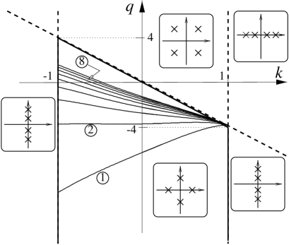
FIG. 1.: The $(k,q)$ parameter plane of the three-wave model (1) – (3). The linear analysis (the results of which are summarized in the inset boxes) shows that ES with $c=0$ may occur only in the region between the solid bold lines. The bundle of curves emanating from the point $(k=1,q=-4)$ are branches of embedded-soliton solutions with $c=0$.

Soliton solutions to Eqs. (1)–(3) are sought in the form

$$v_{1,2}(x,z)=\exp(ikz)\,u_{1,2}(\xi),\;v_{3}(x,z)=\exp(2ikz)\,u_{3}\,,$$ (6)

where $\xi\equiv x-cz$, with $c$ being the walkoff (slope) of the spatial soliton’s axis relative to the light propagation direction $z$. The substitution of (6) into Eqs. (1)–(3) leads to an 8th-order system of ordinary differential equations (ODEs) for the real and imaginary parts of $v_{1,2,3}$ (primes standing for $d/d\xi$):

$$-ku_{1}+i(1-c)u_{1}^{\prime}+u_{2}+u_{3}u_{2}^{\ast} = 0,$$ (7)

$$-ku_{2}-i(1+c)u_{2}^{\prime}+u_{1}+u_{3}u_{1}^{\ast} = 0,$$ (8)

$$-(4k+q)u_{3}+Du_{3}^{\prime\prime}-2icu_{3}^{\prime}+u_{1}u_{2} = 0.$$ (9)

Before looking for ES solutions to the full nonlinear equations, it is necessary to investigate the eigenvalues $\lambda$ of their linearized version, in order to isolate the region in which ESs may exist. Substituting $u_{1},u_{2}\sim\exp(\lambda\xi)$, and $\,u_{3}\sim\exp(2\lambda\xi)$ into Eqs. (6)–(8) and linearizing, one finds that the FH and SH equations decouple in the linearized approximation. The FH equations give rise to a biquadratic characteristic equation,

$$(1-c^{2})^{2}\lambda^{4}+2\left[(1+c^{2})k^{2}-(1-c^{2})\right]\lambda^{2}+(k^{2}-1)^{2}=0\,,$$ (10)

and the SH equation produces another four eigenvalues given by

$$\left[D\lambda^{2}-(4k+q)\right]^{2}+4c^{2}\lambda^{2}=0.$$ (11)

A necessary condition for the existence of ESs is that the eigenvalues given by Eq. (10) have non-zero real parts - this is necessary for the existence of exponentially localized solutions - while the eigenvalues from Eq. (11) should be purely imaginary (otherwise, one will have ordinary, rather than embedded, solitons). This discrimination between the two sets of the eigenvalues is due to the fact that Eqs. (7) and (8) for the FH components are always linearizable, while the SH equation (9) may be nonlinearizable, which opens the possibility for the existence of ESs [5]. As it follows from Eqs. (10) and (11), these two conditions imply

$$k^{2}+c^{2}<1;\;4k+q<c^{2}/D\,.$$ (12)

For the case $c=0$, the parametric region defined by the inequalities (12) is displayed in Fig. 1.

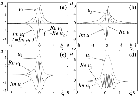
FIG. 2.: Typical examples of the fundamental embedded solitons with the zero walkoff: (a) the ground-state for $k=0$; (b) the same solution for $k=-0.95$; (c,d) the first and eighth “excited states” for $k=0$.

In Ref. [8], numerous ordinary (gap [10]) soliton solutions to the present model have been found by means of a numerical shooting method. To construct ES solutions, we applied the same method to Eqs. (7), (8) and (9), allowing just one parameter to vary. From each ES solution that was found this way, branches of the solutions were continued in the parameters $k,\,q$ and $c$, by means of the software package AUTO [11]. Note that the $c=0$ solutions admit an invariant reduction $u_{2}=-u_{1}^{\ast}$, $\,u_{3}=u_{3}^{\ast}$, which reduces the system to a 4th-order ODE system, thus making numerical shooting feasible.

We confine the analysis to fundamental solitons, which implies that the SH component $u_{3}$ has a single-humped shape (a distinctive feature of gap solitons in the same system is that not only fundamental solitons, but also certain double-humped two-solitons (bound states of two fundamental solitons) appear to be stable [8]). Note that double- and multi-humped ESs must exist too as per a theorem from Ref. [12], but leaving them aside, we will still find a rich structure of fundamental ESs.

FIG. 3.: A diagram of the $c=0$ embedded solitons on the (energy-flux, mismatch) plane. The inset zooms the most interesting part of the diagram.

We begin with a description of the results from the reduced case $c=0$, when an additional scaling allows us to set $D\equiv 1$ without loss of generality. The results are displayed in Figs. 1 – 3. There is a strong evidence for existence of an infinite “fan” of fundamental ES branches. Among them, we define a ground-state soliton as the one which has the simplest internal structure (Fig. 2a). The next “first excited state” differs by adding one (spatial) oscillation to the FH field (Fig. 2c). Adding each time an extra oscillation, we obtain an indefinitely large number of  “excited states” (as an example, see the 8th state in Fig. 2d). We stress, however, that all the “excited states” belong to the class of the fundamental solitons, rather than being bound states thereof.

In Fig. 1, the first nine states (branches) are shown in the $(k,q)$ parametric plane. Note that the whole bundle of the branches originates from the point $(k=1,q=-4)$, which is precisely the intersection of the two lines which limit the existence region of ES (see Eq. (12) with $c=0$). At this degenerate point, the linearization (see above) gives four zero eigenvalues. More branches than those depicted in Fig. 1 have been found, the numerical results clearly pointing towards the existence of infinitely many branches, accumulating on the border $q+4k=0$ of the ES-region. In the accumulation process, each $u_{3}$ component is successively wider, while the $u_{1,2}$ ones have more and more internal oscillations.

Since $k$ is an arbitrary propagation constant, from physical grounds, the results obtained for the $c=0$ solutions are better summarized in terms of energy flux $E$ vs. mismatch $q$ (Fig. 3). Note that all the branches shown in Fig. 3 really terminate at their edge points, which exactly correspond to hitting the boundary $k=-1$, see Fig. 1. It is also noteworthy that all the solutions are exponentially localized, except at the edge point $k=-1$, where a straightforward consideration of Eqs. (7)–(9) demonstrates that, in this case, ES are weakly (algebraically) localized as $|x|\rightarrow\infty$ (cf. Fig 2b):

$\displaystyle\begin{array}[]{c}u_{1}\approx\sqrt{-(4k+q)}|x|^{-1},\,u_{2}\approx(1/2)\sqrt{-(4k+q)}|x|^{-2},\\ u_{3}\approx x^{-2}\,.\end{array}$

Finally, we observe from Figs. 1 and 3 that the first “excited-state” branch has a remarkable property that it corresponds to a nearly constant value of $q$. This means that while, generally, ES are isolated (codimension-one) solutions for fixed values of the physical parameters, this branch is nearly generic, existing in a narrow interval of the $q$-values between $-4.0$ and $-3.74$.

III Walking Solitons

We now turn to ESs with $c\neq 0$, i.e., walking ones. These were sought for systematically by returning to the full 8th-order-ODE model and allowing the AUTO package to detect bifurcations (of the pitchfork type), while moving along branches of the $c=0$ solutions. It transpires that all the bifurcating branches have $c\neq 0$, i.e., they are walking ESs. Such solutions are of codimension-two in the parameter space (i.e., the solutions can be represented by curves $k(q)$, $c(q)$), which can be established by a simple counting argument after noting that the 8th-order linear system has two pairs of pure imaginary eigenvalues. Alternatively, the walking ESs can be represented, in terms of the energy flux and momentum (see Eqs. (4) and (5)), by curves $E(q)$ and $P(q)$. We present results only for the walking solutions which bifurcate from the ground and first excited $c=0$ states, while other walking ESs can also be readily found.

It was found that the ground-state branch has exactly two bifurcation points, giving rise to two distinct walking-ES solution branches (up to a symmetry). These new branches are shown, in terms of the most physically representative $c(q)$ and $E(q)$ dependences, in Fig. 4. Note that they, eventually, coalesce and disappear. As the inset to Fig. 4b shows, they disappear via a tangent (fold, or saddle-node) bifurcation.

The first excited state has three bifurcation points. One of them gives rise to a short branch of walking ESs that terminates, while two others appear to extend to $q=-\infty$ (their ostensible “merger” in Fig. 5 is an artifact of plotting). It is known that, in the large-mismatch limit $q\rightarrow-\infty$, the present three-wave model with the quadratic nonlinearity goes over into a modified Thirring model with cubic nonlinear terms [13]. This suggests that the latter model may also support ES. However, consideration of this issue is beyond the scope of the present work.

FIG. 4.: Two branches of “walking” ($c\neq 0$) embedded solitons bifurcating from the ground-state $c=0$ branch: (a) the walkoff $c$, and (b) the energy flux $E$ vs. the mismatch $q$. The horizontal segment in (a) shows the branch of the $c=0$ solutions. The inset in (b) shows that the two branches meet and disappear via a typical tangent bifurcation.

Fig. 4 clearly shows that, in a certain interval of the mismatch parameter $q$, the system gives rise to a multistability, i.e., coexistence of different types of spatial solitons in the planar optical waveguide (for instance, taking account of the fact that each $c\neq 0$ branch has symmetric parts with the opposite values of $c$, we conclude that there are five coexisting solutions at $q$ taking values between about $-8$ and $-11$). This situation is of obvious interest for applications, especially in terms of all-optical switching [9]. Indeed, switching from a state with a larger value of the energy flux to a neighboring one with a smaller flux can be easily initiated by a small localized perturbation, in view of the above-mentioned one-sided semistability of ES, shown in a general form in [5]. Such a switching perturbation can be readily made controllable and movable if created by a laser beam launched normally to the planar waveguide and focused at a necessary spot on its surface [14]. Switching between the two branches with $c\neq 0$ can be quite easy to realized too, due to small energy-flux and walkoff/momentum differences between them, see Fig. 4.

IV Conclusion

To conclude the analysis, it is necessary to estimate the actual size of the relevant physical parameters. This is, in fact, quite easy to do, as there is no essential difference in the estimate from that which was presented in Ref. [8] for the ordinary solitons in exactly the same model. This means that a diffraction length $\sim 1$ cm is expected for the SH component, and, definitely, the diffraction lengths for the FH components, which are subject to the strong Bragg scattering, will be no larger than that. Thus, a sample with a size of a few cm may be sufficient for the experimental observation of ESs. The sample may be an ordinary planar quadratically nonlinear waveguide with a set of parallel scores written on it. The other parameters, such as the power of the laser beam that generates the solitons, etc., are expected to be the same as in the usual experiments with the spatial solitons [9]. As concerns the weak semi-instability of ESs, it may be of no practical consequence for the experiment, as it would manifest itself only in a much larger sample. In this connection, it may be relevant to mention that, strictly speaking, the usual spatial solitons observed in numerous experiments are all unstable (e.g., against transverse perturbations) in the usual (linear) sense, but the instability has no room to develop in real experimental samples.

Finally, we see from Figs. 4 and 5 that the maximum walkoff that ESs can achieve is, in the present notation, slightly smaller than $1$. According to the geometric interpretation of the underlying equations (1) - (3) (see details in the original work [8]), this implies that the maximum size of the misalignment angle between the propagation direction and the axis of the spatial soliton may be nearly the same as the (small) angle between the Poynting vectors of the two FH waves and that of the SH wave.

To summarize the work, we have found a rich spectrum of isolated solitons residing inside the continuous spectrum in a simple model of the three-wave spatial interaction in a second-harmonic-generating planar optical waveguide equipped with a quasi-one-dimensional Bragg grating. An infinite sequence of fundamental embedded solitons were found. They differ by the number of internal oscillations. The embedded solitons are localized exponentially, except for a limiting degenerate case, when they become algebraically localized. Branches of the zero-walkoff spatial solitons give rise, through bifurcations, to several branches of walking solitons. The structure of the bifurcating branches provides for a multistable configuration of the spatial optical solitons. This may find straightforward applications to all-optical switching.

REFERENCES

- [1] J.P. Boyd, Weakly Nonlocal Solitary Waves and Beyond-All-Orders Asymptotics (Kluwer: Dodrecht, Boston, London, 1998).
- [2] D.J. Kaup, T.I. Lakoba, and B A. Malomed, J. Opt. Soc. Am. B 14, 1199 (1997).
- [3] A.R. Champneys and M.D. Groves, J. Fluid Mech. 342, 199 (1997). R. Grimshaw and P. Cook, in Hydrodynamics eds. A.T. Chang, J.H. Lee and D.Y.C. Leung (Balkema: Rotterdam, 1996)
- [4] A.R. Champneys, B.A. Malomed, and M.J. Friedman, Phys. Rev. Lett. 80, 4169 (1998).
- [5] J. Yang, B.A. Malomed, and D.J. Kaup, Phys. Rev. Lett., in press.
- [6] S. Trillo, A.V. Buryak, and Y.S. Kivshar, Opt. Comm. 122, 200 (1996); O. Bang, Y.S. Kivshar, and A.V. Buryak, Opt. Lett. 22, 1680 (1997).
- [7] J. Yang, A.R. Champneys, B.A. Malomed, and D.J. Kaup, to be published.
- [8] W.C.K. Mak, B.A. Malomed, and P.L. Chu. Phys. Rev. E 58, 6708 (1998).
- [9] G.I. Stegeman, D.J. Hagan, and L. Torner, Opt. Quantum Electron. 28, 1691 (1996).
- [10] C.M. de Sterke and J.E. Sipe, Progr. Opt. 33, 203 (1994). Lett. Nuovo Cimento 20, 325 (1996).
- [11] E.J. Doedel, A.R. Champneys, T.R. Fairgrieve, Yu.A. Kuznetsov, B. Sanstede, and W. Wang, AUTO97 Continuation and Bifurcation Software for Ordinary Differential Equations, 1997. Available by anonymous ftp from ftp.cs.concordia.ca, directory pub/doedel/auto.
- [12] A. Mielke, P. Holmes and O. O’Reilly, J. Dynamics Diff. Eq. 4, 95 (1992)
- [13] S. Trillo, Opt. Lett. 21, 1732 (1996).
- [14] B.A. Malomed, Z.H. Wang, P.L. Chu, and G.D. Peng, J. Opt. Soc. Am. B 16, 1197 (1999).