Moving Embedded Solitons

Abstract

The first theoretical results are reported predicting moving solitons residing inside (embedded into) the continuous spectrum of radiation modes. The model taken is a Bragg-grating medium with Kerr nonlinearity and additional second-derivative (wave) terms. The moving embedded solitons (ESs) are doubly isolated (of codimension 2), but, nevertheless, structurally stable. Like quiescent ESs, moving ESs are argued to be stable to linear approximation, and semi-stable nonlinearly. Estimates show that moving ESs may be experimentally observed as $\sim$10 fs pulses with velocity $\leq 1/10$th that of light.

PACS: 42.81.Dp; 42.79.Dj; 42.50.Rh; 03.40.Kf

Recent studies have revealed a novel type of soliton (“solitary wave” is more accurate since we do not assume integrability) that is embedded into the continuous spectrum, i.e., the soliton’s internal frequency is in resonance with linear (radiation) waves. Generally, such a soliton should not exist, one finding instead a “quasi-soliton” with non-vanishing oscillatory tails (radiation component) [1]. Nevertheless, bona fide (exponentially decaying) solitons can exist as codimension-one solutions if, at discrete values of the (quasi-)soliton’s internal frequency, the amplitude of the tail exactly vanishes, while the soliton remains embedded into the continuous spectrum. This requires the spectrum of the corresponding linearized system to consist of (at least) two branches, one corresponding to exponentially localized solutions, and the other to radiation modes. In terms of the travelling-wave ordinary differential equations (ODEs), the origin must be a saddle-centre equilibrium.

Examples of such embedded solitons (ESs) were found in water-wave models [2] and in several nonlinear-optical ones, e.g., a Bragg grating with dispersion and/or diffraction terms [3], and second-harmonic generation (SHG) in the presence of a self-defocusing Kerr nonlinearity ([4, 5]). The term “ES” was proposed in Ref. [4].

It is relevant to stress that ESs, although they are isolated solutions, are not structurally unstable. Indeed, a small change of the model’s parameters will slightly change the location of ES (e.g., its energy and momentum, see below), but will not destroy it, which is quite obvious from the already published results [2, 4]. In this respect, they may be called generic solutions of codimension one.

ESs are interesting for several reasons, firstly because they frequently appear when higher-order (singular) perturbations are added to the system, which may completely change its soliton spectrum (see e.g. [3]). Secondly, optical ESs may have a potential for applications, just because they are isolated solitons rather than members of continuous families. Finally, and most crucially for their physical applications, it appears that ESs are semi-stable objects. That is, as is proven in Ref. [4] analytically in a fairly general form, and checked numerically for a particular model combining SHG (quadratic) and Kerr (cubic) nonlinearities, ESs are fully stable in the linear approximation, but are subject to a slowly growing (sub-exponential) one-sided nonlinear instability (see below). The analytical proof of the semistability presented in Ref. [4] applies to any system that gives rise to ESs. As for the one-sided nonlinear instability, its development depends on values of the system’s parameters; in some cases, it may be developing so slowly that ES, to all practical purposes, may be regarded as a fully stable object [6].

An issue important both for applications and by itself is whether moving ESs (ones with non-zero momentum) may occur in systems where they cannot be generated by a straightforward transformation, like Galilean or Lorentz transformation (the absence of the corresponding invariance is typical for nonlinear-optical systems). The objective of the present work is to search for moving ESs in a physically important system, viz., a nonlinear Bragg-grating model similar to that introduced in [3], which takes into account second-derivative (wave) terms. In fact (see below), this system has a broader physical purport than was originally assumed in [3]. The absence of the Galilean or Lorentzian invariance in it is obvious because there is a reference frame in which the Bragg grating is quiescent. Although exact solutions for moving solitons are available in the traditional version of this model, which neglects the second-derivative terms [7, 8], they can be obtained by the Lorentz transformation from the quiescent solitons only in the limiting case of the Thirring model [9], which is completely integrable [10].

We start from a system of partial differential equations (PDEs) governing evolution of right- ($u(x,t)$) and left- ($v(x,t)$) traveling waves that continuously transform into each other due to the resonant reflection on the grating:

$$iu_{t}+iu_{x}+(2k)^{-1}\left(u_{xx}-u_{tt}\right)+\left(\sigma|u|^{2}+|v|^{2}\right)u+v = 0,$$

$$iv_{t}-iv_{x}+(2k)^{-1}\left(v_{xx}-v_{tt}\right)+\left(\sigma|v|^{2}+|u|^{2}\right)v+u = 0.$$

Here, the cubic and linear cross-coupling terms account, respectively, for nonlinear cross-phase modulations and Bragg scattering. The most natural physical value of the relative self-modulation coefficient $\sigma$ is $1/2$ , but it will be quite useful to keep $\sigma$ as an arbitrary positive parameter. Note that Eqs. (1) and (2) have three natural integrals of motion: the energy (norm) and momentum,

$$E\equiv\int_{-\infty}^{+\infty}\left[|u(x)|^{2}+|v(x)|^{2}\right]dx\,,\,\,P\equiv i\int_{-\infty}^{+\infty}\left(u_{x}^{\ast}u+v_{x}^{\ast}v\right)dx\,,$$

and a Hamiltonian, an expression for which is obvious.

The energy plays a crucial role in analyzing ES stability [4], as ESs are isolated solutions with uniquely determined values of the energy. Hence, any small perturbation which slightly increases the ES’s energy is safe, while a perturbation that slightly decreases the energy triggers a slow (sub-exponential) decay into radiation. So in this sense, the weak instability of an ES is one-sided, as mentioned above, and in some cases it may be extremely weak [6].

Eqs. (1) and (2) can be derived from the Maxwell’s equations for a nonlinear medium, assuming a superposition of two counter-propagating electromagnetic waves, $u(x,t)\,\exp(ikx-i\omega t)$ and $v(x,t)\,\exp(-ikx-i\omega t)$, where the wavenumber $k$ and frequency $\omega$ are related by the linear dispersion relations (disregarding their Bragg coupling), the functions $u(x,t)$ and $v(x,t)$ being slowly varying as compared to the carrier waves. Taking (for simplicity) a medium whose temporal dispersion may be neglected, and setting $c_{0}\equiv 1$ (hence, $\omega=k$), one derives, to lowest order in the small parameter $1/2k$, Eqs. (1) and (2) without the second-derivative terms, i.e., a standard model of the Bragg reflector filled by a Kerr-nonlinear medium [7, 8]. As shown in [3], the second-derivative (wave) terms which come in at the next order drastically alter the soliton spectrum of the model (since this is a singular perturbation, increasing the order of the PDEs). In an experiment (see below for an estimate of physical parameters), the effect of the additional terms may be seen if the observation time and/or propagation distance are long enough.

Solitons are solutions of the form

$$u(x,t)=\exp(-i\Delta\omega t)\,U(\xi),\;v(x,t)=\exp(-i\Delta\omega t)\,V(\xi),$$

where $\xi\equiv x-vt$, $v$ is the soliton’s velocity, and $\Delta\omega$ is a frequency shift. The substitution of this expression into Eqs. (1) and (2) yields the ODEs,

$$\chi U+i(1-c)U^{\prime}+DU^{\prime\prime}+\left(\sigma|U|^{2}+|V|^{2}\right)U+V=0,$$ (1)

$$\chi V-i(1+c)V^{\prime}+DV^{\prime\prime}+\left(\sigma|V|^{2}+|U|^{2}\right)V+U=0,$$ (2)

where $\chi\equiv\Delta\omega+\left(\Delta\omega\right)^{2}/2k$, the effective velocity is $c\equiv(1+\Delta\omega/k)v$, and an effective dispersion coefficient is $D\equiv\left(1-v^{2}\right)/2k$.

In [3] the same ODEs were derived in two more special physical contexts: (i) a nonlinear Bragg-grating medium incorporating spatial-dispersion effects and (ii) spatial evolution (i.e. with $t$ realized as a propagation coordinate) in a planar waveguide equipped with a Bragg grating in the form of a set of parallel scores, taking ordinary diffraction into regard. While all these systems are described Eqs. (1) and (2), the new physical interpretation of the model as describing the usual Bragg-grating system with the wave terms taken into regard, seems most fundamental.

To look for ES solutions, we must first satisfy the necessary condition, viz., that the linearization of the ODEs should be of the saddle-centre type. That is, at least one pair of eigenvalues must be purely imaginary (otherwise, we are dealing with regular, i.e., non-embedded, solitons), and at least one pair must not be purely imaginary (otherwise, there can be no exponentially decaying tails). Hence the region in which ESs may exist may be delineated by substituting $U,V\sim\exp(\lambda\xi)$ into the linearized equations and solving the resulting eighth-order algebraic equation for $\lambda$ numerically. It is easy to demonstrate that purely real or imaginary eigenvalues always appear in pairs, and complex eigenvalues in quadruples: if $\lambda$ is an eigenvalue, then so are $\pm\lambda$ and $\pm\lambda^{\ast}$.

We do not display here the full results for the linear spectrum, as they are rather cumbersome. But note that in the quiescent case ($c=0$) the spectrum is expressible in a closed form [3], and the region in the $(\chi,D)$ -plane where ESs may occur is just $|\chi|<1$, $D>0$. When $c\neq 0$, these borders to the saddle-centre region of $(c,\chi,D)$-space retain exactly the same meaning (but there appear additional bounding surfaces that, in fact, are not encountered by any of the ES branches that we have computed, see below). Two degenerate limits of special interest are $\chi\rightarrow+1$ (the soliton amplitude going to zero) and $\chi\rightarrow-1$ (a smooth transition into a regular soliton).

Eqs. (1) and (2) were numerically solved by means of the same techniques as used in Ref. [3]. That is, a two-point boundary-value problem is posed on a long but finite $x$-interval, with boundary conditions chosen to place the solution in the stable or unstable eigenspaces at the endpoints [11]. The boundary-value problem can be formulated so that the imaginary parts of $A(\xi)$ and $B(\xi)$ are always even functions, while the real parts are odd. Using these reversibility conditions at the midpoint of the soliton, the numerical problem was posed more simply on the half $x$-interval. Only fundamental (single-humped) solitons were sought because, although multi-humped ESs may easily exist, they have no chance to be stable [4]. Continuation of the solutions corresponding to variation of relevant parameters was carried out by means of the well-known software package AUTO [12].

Quiescent ESs (with $c=0$) in the present model were found in Ref. [3] , aided by the observation that, at $c=0$, Eqs. (1) and (2) admit an invariant reduction $V\equiv U^{\ast}$, thus reducing the system’s order from $8$ to $4$. The result was that there exist exactly three different branches of quiescent ES solutions. Because ESs exist at isolated values of the energy, each branch can be represented by a curve $E(D)$ in three separate $D$-intervals (which overlap). Equivalently, the curves can be represented as $D(\chi)$ for $-1<\chi<1$.

To the best of our knowledge, moving ESs have never been found before in any model. Our numerical solution of the full system (1) and (2) has demonstrated that an arbitrary quiescent ES cannot be directly continued into a moving one. Nevertheless, moving ESs exist, but they turn out to be of codimension two, i.e., they are double-isolated, both in the energy and in the momentum (but, nevertheless, they remain structurally stable objects). In other words, a moving ES is described by curves $E(D)$ and $P(D)$. Equivalently, such curves may be represented in the $(D,c,\chi)$-space, an important characteristic of a moving soliton being its velocity $c$. The mathematical reason for the codimension being two is that, for the 8th-order model, there are two pairs of eigenvalues on the imaginary axis (rather than one pair for the reduced 4th-order model satisfied by the quiescent ESs). A simple count of dimensions of the unstable manifold and symmetric set of the reversibility then yields that to force their intersection (implying the existence of a solitary wave) requires two parameters to be varied.

The results were found to be sensitive to the value of $\sigma$ (see Eqs. (1) and (2)); note that in the case $c=0$, $\sigma$ is trivially scaled out [3]. The case at which it was easiest to find moving ESs was $\sigma=0$. The results obtained for this case are summarized in Fig. 1, which shows that each branch of quiescent ES solutions gives rise, through a pitchfork bifurcation occurring at some special value of $D$, to two mutually symmetric branches of moving ESs. In Fig. 1 (and Fig. 2 below), we cut each branch at points where they go over into regular (non-ES) solitons (at $\chi=-1$). Also, we have not depicted the quiescent branches all the way up to $\chi=+1$ due to numerical difficulties occurring in this singular limit.

In the case $\sigma=0$, it was easy to find additional branches of moving-ES solutions that are not connected to the quiescent ones. Only one such disjoint branch is shown in Fig. 1. It is quite interesting that this disjoint branch persists for all $|\chi|<1$ without ever bifurcating from a quiescent ES.

Although the case $\sigma=0$ exactly corresponds to the Thirring model [9], it has no straightforward meaning for optical systems. Therefore, we now focus attention on the most physically relevant case $\sigma=1/2$. In this case, only one branch of quiescent ESs, corresponding to the smallest values of $D$, gives rise, through a bifurcation, to branches of moving solitons. Scanning the parameter space has not yielded any disjoint branch, cf. Fig. 1. This case is shown, in various forms, in Fig. 2. It is interesting, in particular, that the momentum of the moving ESs vanishes at a nonzero value of the velocity, exactly (within the accuracy of the numerical calculation) as it passes into the non-embedded region ($\chi<-1$), see Fig. 2b.

The plot that simultaneously shows the energy of the moving ESs and of the coexisting quiescent ESs (Fig. 2c) is especially important. Following the lines of the stability analysis of ESs developed in [4], we can draw conclusions concerning the stability of both types of the ES solitons. The analysis developed in [4] shows that a small perturbation which decreases the energy of an isolated ES solution would trigger a continual decrease of energy via emission of radiation. In the model considered in Ref. [4], this would eventually lead to complete decay of ESs into radiation. However, in the present case, a moving ES is likely to shed not only its energy, but also momentum, and eventually to decay into a quiescent ES. Because this instability is weak (sub-exponential), we may view the full set of ESs as a tri-stable system, in which transitions from ESs moving at the velocities $\pm c$ to the quiescent one are possible.

The latter configuration has a potential for use in optical-memory devices. If an incoming moving ES represents a new bit of information, its radiation-mediated transition into a quiescent ES can be triggered by a specially inserted perturbation (e.g., a localized spatial inhomogeneity, which can be readily made switchable and movable if created by a laser beam focused on a spot in the medium [13]). Thus, the incoming bit could be captured and stored in the memory.

Further numerical explorations have revealed that the single branch of moving ESs existing at $\sigma=1/2$ is not a continuation in $\sigma$ of any branch existing at $\sigma=0$; actually, the continuations of all those branches terminate between $\sigma=0.1$ and $\sigma=0.2$, but a new branch appears in the same region which continues to that found at $\sigma=1/2$. Continuation of this branch to larger values of $\sigma$ (the case $\sigma\rightarrow\infty$ has a physical application to dual-core optical fibers or waveguides) shows that it terminates at $\sigma\approx 1.645$. Additional moving ESs exist at still larger values of $\sigma$ (e.g., at $\sigma=8.7$), but none was found for $\sigma>10$.

Finally, one can estimate the values of the physical quantities for direct experimental observation of these ESs in a Bragg-grating medium. First of all, it is relevant to note that, as Fig. 2a clearly shows, the velocity at which moving ESs may be observed includes all the values from $0$ up to $\sim(1/10)c_{0}$, which is an interesting result by itself, and is quite convenient for the experiment.

A parameter which is crucial for the physical relevance of the model characterizes the relative smallness of the wave (second-derivative) terms in Eqs. (1) and (2). Obviously, it is $D/W$, $W$ being the ES width. From the data presented in the insets to Figs. 1 and 2, it follows that this parameter takes a nearly constant value, $\sim 0.1$, along a moving-ES branch. On the other hand, from the underlying PDEs, it follows that, in terms of physical quantities, the same smallness parameter is $\sim\lambda/4\pi c_{0}T$, where $\lambda\equiv 2\pi/k$ is wavelength of light, and $T$ is the temporal width of the pulse. Taking $\lambda\sim 1.5$ $\mu$m, and equating the two expressions for the same smallness, we conclude that one needs $T\sim 10$ fs.

In recently reported experiments in which the temporal solitons were first observed in a Bragg-grating medium $T$ was much larger; $\sim 10$ ps [14]. However, much shorter pulses can be produced by means of existing experimental techniques. For instance, the first experimental observation of temporal solitons in second-harmonic-generating media used pulses of width $58$ ps [15]. Moreover, generation of stable pulses with the temporal duration ${}_{\sim}^{<}\,5$ fs, which contain just two optical cycles, has been successfully demonstrated in recent years (see, e.g., Ref. [16] and references therein). This circumstance suggests a possible link between ESs and rapidly developing studies of the ultrashort few-cycle optical pulses.

We appreciate valuable discussions with M.J. Friedman, D.J. Kaup, Y.S. Kivshar, and J. Yang. The stay of B.A.M. at the University of Bristol was supported by a Benjamin Meaker visiting professorship.

Figure Captions

Figure 1: The solution branches of the quiescent and moving (dotted amd solid lines) embedded solitons in the case $\sigma=0$; squares show bifurcations, circles label points. (a) The velocity vs. the effective dispersion coefficient $D$. The insets show typical examples of the solutions on the first branch. (b) The effective frequency $\chi$ vs. $D$.

Figure 2: Various representations of the single branch of the moving embedded solitons existing in the physically relevant case, $\sigma=1/2$: (a) the same as in Fig. 1; (b) the momentum vs. $D$; (c) the energy vs. $D$, with insets showing the solutions at labeled points. The quiescent solitons branch from which the moving-soliton branch bifurcates is also shown.

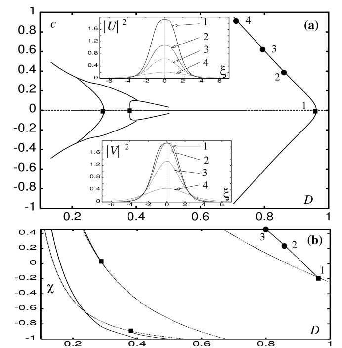
Figure 1:

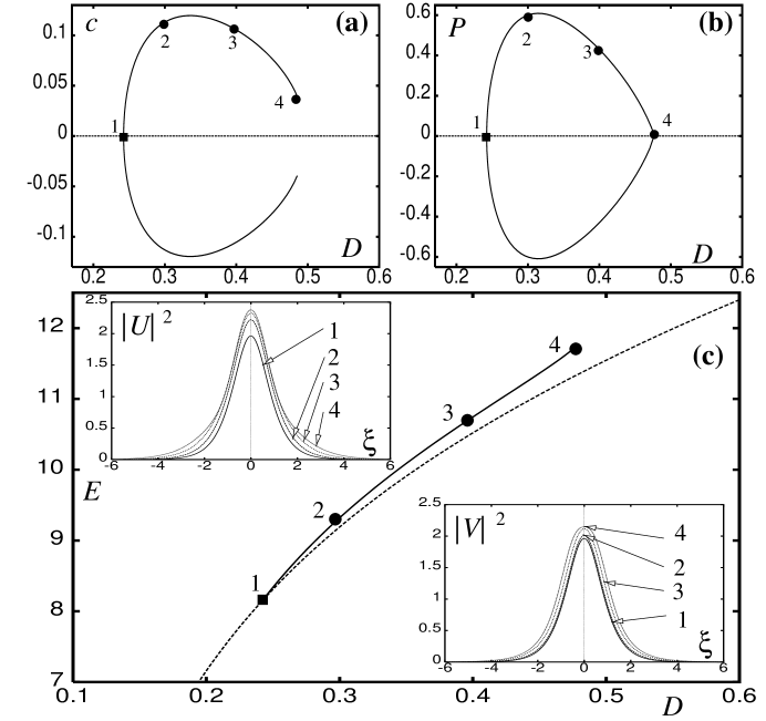
Figure 2:

References

- [1] J.P. Boyd, Weakly Nonlocal Solitary Waves and Beyond-All-Orders Asymptotics (Kluwer: Dodrecht, Boston, London, 1998).
- [2] A.R. Champneys and M.D. Groves, J. Fluid Mech. 342, 199 (1997). R. Grimshaw and P. Cook in Hydrodynamics eds. A.T. Chang, J.H. Lee and D.Y.C. Leung (Balkema: Rotterdam, 1996)
- [3] A.R. Champneys, B.A. Malomed, and M.J. Friedman, Phys. Rev. Lett. 80, 4169 (1998).
- [4] J. Yang, B.A. Malomed and D.J. Kaup, “Embedded solitons in second-harmonic-generating systems”, Phys. Rev. Lett., in press
- [5] S. Trillo, A.V. Buryak, and Y.S. Kivshar, Opt. Comm. 122, 200 (1996); O. Bang, Y.S. Kivshar, and A.V. Buryak, Opt. Lett. 22 , 1680 (1997).
- [6] J. Yang, A.R. Champneys, B.A. Malomed, and D.J. Kaup, to be published.
- [7] D.N. Christodoulides and R.I. Joseph, Phys. Rev. Lett. 62, 1746 (1989); A. Aceves and S. Wabnitz, Phys. Lett. A 141, 37 (1989).
- [8] C.M. de Sterke and J.E. Sipe, Progr. Opt. 33, 203 (1994).
- [9] W.E. Thirring, Ann. Phys. (N.Y.) 3, 91 (1958).
- [10] A.V. Mikhailov, JETP Lett. 23, 320 (1976); D.J. Kaup and A.C. Newell, Lett. Nuovo Cimento 20, 325 (1996).
- [11] E.J. Doedel, M.J. Friedman, and B.I. Kunin, Numer. Algorithms 14, 103 (1997); A.R. Champneys, Yu.A. Kuznetsov, and B. Sanstede, Int. J. Bifurcation Chaos 6, 867 (1996).
- [12] E.J. Doedel, A.R. Champneys, T.R. Fairgrieve, Yu.A. Kuznetsov, B Sanstede, and W. Wang, AUTO97 Continuation and Bifurcation Software for Ordinary Differential Equations, 1997. Available by anonymous ftp from ftp.cs.concordia.ca, directory pub/doedel/auto.
- [13] B.A. Malomed, Z.H. Wang, P.L. Chu, and G.D. Peng, J. Opt. Soc. Am. B 16, 1197 (1999).
- [14] B.J. Eggleton, R.E. Slusher, C.M. de Sterke, P.A. Krug, and J.E. Sipe, Phys. Rev. Lett. 76, 1627 (1996).
- [15] P. Di Trapani, D. Caironi, G. Valiulis, A. Dubietis, R. Danielius, and A. Piskarskas, Phys. Rev. Lett. 81, 570 (1998).
- [16] V.P. Kalosha and J. Herrmann, Phys. Rev. Lett. 83, 544 (1999).