Atomic dynamics in evaporative cooling of
trapped alkali atoms in strong magnetic fields

Abstract

We investigate how the nonlinearity of the Zeeman shift for strong magnetic fields affects the dynamics of rf field induced evaporative cooling in magnetic traps. We demonstrate for the ⁸⁷Rb and ²³Na $F=2$ trapping states with wave packet simulations how the cooling stops when the rf field frequency goes below a certain limit (for the ⁸⁵Rb $F=2$ trapping state the problem does not appear). We examine the applicability of semiclassical models for the strong field case as an extension of our previous work [Phys. Rev. A 58, 3983 (1998)]. Our results verify many of the aspects observed in a recent ⁸⁷Rb experiment [Phys. Rev. A 60, R1759 (1999)].

I Introduction

Bose-Einstein condensation of alkali atoms in magnetic traps was first observed in 1995 [1], and since then the development in related research has been been very swift. Typically the hyperfine state used in the alkali experiments is the $F=1$ state, although condensation has been demonstrated for the ⁸⁷Rb $F=2$ case as well [2]. The trapping of atoms is based on moderate, spatially inhomogeneous magnetic fields, which create a parabolic, spin-state dependent potential for spin-polarised atoms, as shown in Fig. 1(a). For slowly moving atoms the trapping potential depends on the strength of the magnetic field $B$ but not on its direction [3]. In practice the field is dominated by a constant bias field $\vec{B}_{\rm bias}$, which eliminates the Majorana spin flips at the center of the trap.

In evaporative cooling the hottest atoms are removed from the trap and the remaining ones thermalise by inelastic collisions. This leads to a decrease in temperature of the atoms remaining in the trap [4, 5, 6]. Continuous evaporative cooling requires adjustable separation into cold and hot atoms. This is achieved by inducing spin flips with an oscillating (radiofrequency) magnetic field, which rotates preferably in the plane perpendicular to the bias field [6, 7]. In the limit of linear (weak) Zeeman effect the rf field couples the adjacent magnetic states $M_{F}$ resonantly at the spatial location determined by the field frequency [Fig. 1(a)]. Hot atoms oscillating in the trap can reach the resonance point and exit the trap after a spin flip to a nontrapping state. Using the rotating wave approximation we can eliminate the rf field oscillations, and obtain the curve crossing description of resonances [Fig. 1(b)].

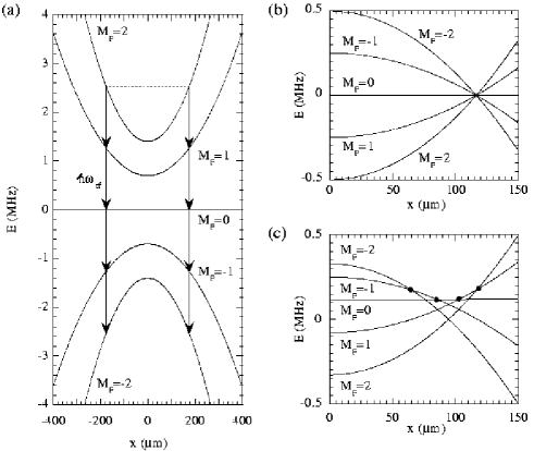
FIG. 1.: The magnetic trap potentials for spin-polarised ⁸⁷Rb ($F=2$). (a) The spin flips that lead to evaporation are achieved by an rf field induced multistate transition at a specific spatial distance from the trap center. Here $B_{0}=0.0001$ T. (b) In the curve crossing description the resonances appear as degeneracies. Here $B_{0}=0.0001$ T. (c) For strong fields the multistate crossing transforms into a sequence on two-state crossings between adjacent $M_{F}$ states. Here $B_{0}=0.0020$ T. The circles mark those crossings where the involved adjacent $M_{F}$ states are also coupled. In (b) and (c) we have $\nu_{\rm rf}=0.25$ MHz+$\nu_{0}$.

The dynamics of atoms as they move past the resonance point can be described with a simple semiclassical model [8], which has been shown to agree very well with fully quantum wave packet calculations [3]. The model, however, can be applied only if the resonances between adjacent $M_{F}$ states occur at the exactly same distance from the trap center. When the nonlinear terms dominate the Zeeman shifts, the situation changes, as shown in Fig. 1(c). The adjacent resonances become separated and one expects to treat the evaporation as a sequence of independent Landau-Zener crossings as suggested by Desruelle et al. in connection with their recent ⁸⁷Rb experiment [9]. We show that there is an intermediate region where off-resonant two-photon transitions from the $M_{F}=2$ state to the $M_{F}=0$ state, demonstrated in Fig. 2, play a relevant role.

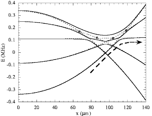
FIG. 2.: The adiabatic potentials (solid lines) and bare $M_{F}$ states (dotted lines) for ²³Na at $B_{0}=0.0010$ T, with rf field coupling $\Omega=(2\pi)20$ kHz. The arrow indicates the semiadiabatic process for transfer from the $M_{F}=2$ state to the $M_{F}=0$ state. Alternatively one can describe the process as an off-resonant two-photon transition.

In general there is a competition between the adiabatic following of the eigenstates (solid lines in Fig. 2), which leads to evaporation, and nonadiabatic transitions which force the atoms to stay in the trapping states. In ²³Na the nonadiabatic transitions can lead to highly inelastic collisions [3].

In the experiment by Desruelle et al. it was found that for a strong bias field the nonlinear Zeeman shifts remove some resonances completely, thus making it impossible to make a spin flip to a nontrapping state. Our calculations confirm this observation. We also show that although evaporation could continue via off-resonant multiphoton processes, such a process is not practical. The stopping of evaporation at some finite temperature occurs for the ⁸⁷Rb and ²³Na $F=2$ trapping states, but not e.g. for the ⁸⁵Rb $F=2$ trapping state.

In Sec. II we write down the formalism for the Zeeman shifts and show the basic properties of the field-dependent trapping potentials. We describe the fully quantum wave packet approach and corresponding semiclassical theories in Sec. III, present and discuss the results in Sec. IV, and summarize our work in Sec. V.

II The Zeeman structure

A ²³Na and ⁸⁷Rb

The Zeeman shifts can not be derived properly in the basis of the hyperfine states (labelled by $F$ and $M_{F}$) [10, 11, 12]. We need to consider the atom-field Hamiltonian in the $(I,J)$ basis:

$$H=A\vec{I}\cdot\vec{J}+CJ_{z}+DI_{z},$$ (1)

where $\vec{I}$ and $\vec{J}$ are the operators for the nuclear and total electronic angular momentum, respectively. The first term describes the hyperfine coupling; $E_{\rm hf}=h\nu_{\rm hf}=2A$, where $E_{\rm hf}$ is the hyperfine splitting between the $F=1$ and $F=2$ states. Here $\nu_{\rm hf}=1772$ MHz for ²³Na and $\nu_{\rm hf}=6835$ MHz for ⁸⁷Rb.

The magnetic field dependence arises from the two other terms, with $C=g_{J}\mu_{B}B$ and $D=-\alpha\mu_{N}B$, where the Bohr magneton is $\mu_{B}=e\hbar/2m_{e}$, the nuclear magneton is $\mu_{N}=e\hbar/2m_{p}$, and the Lande factor is $g_{J}=2$. Here $\alpha=2.218$ for ²³Na and $\alpha=2.751$ for ⁸⁷Rb. But $\mu_{B}/\mu_{N}\sim 1000$, and in fact we can omit the third term in Eq. (1).

For ²³Na and ⁸⁷Rb we have $I=3/2$ and $J=1/2$ (leading to $F=1$ or $F=2$ with $\vec{F}=\vec{I}+\vec{J}$). Our state basis is formed by the angular momentum states labelled with the magnetic quantum number pairs $(M_{I},M_{J})$. When we evaluate the matrix elements of $H$ [using the relation $\vec{I}\cdot\vec{J}=I_{z}J_{z}+\frac{1}{2}(I_{+}J_{-}+I_{-}J_{+})$], the states that correspond to the same value of $M_{F}=M_{I}+M_{J}$ form subsets of mutually coupled states. By diagonalising the Hamiltonian we obtain its eigenstates. The states which correspond to the $F=2$ state in the $B\rightarrow 0$ limit (labelled with $M_{F}$) have the energies $E_{\rm M_{F}}$:

$$E_{+2} = \frac{1}{2}C,$$ (2)

$$E_{+1} = \frac{1}{2}\sqrt{4A^{2}+2AC+C^{2}}-A,$$ (3)

$$E_{0} = \frac{1}{2}\sqrt{4A^{2}+C^{2}}-A,$$ (4)

$$E_{-1} = \frac{1}{2}\sqrt{4A^{2}-2AC+C^{2}}-A,$$ (5)

$$E_{-2} = -\frac{1}{2}C.$$ (6)

These energies have been normalised to the energy of the $F=2$ state for $B=0$. In Fig. 3(a) and (b) we show the Zeeman shifts for all hyperfine ground states of ²³Na and ⁸⁷Rb, but normalised to the ground state energy in the absence of hyperfine structure. For small magnetic fields ($B\ll$ 1 T) we get

$$E_{\rm M_{F}}\simeq E_{\rm hf}[\varepsilon M_{F}+(4-M_{F}^{2})\varepsilon^{2}],$$ (7)

where $\varepsilon=\mu_{B}B/(2E_{\rm hf})$. In terms of $F$ and $M_{F}$ the linear Zeeman shift is $E_{\rm M_{F}}=g_{F}\mu_{B}BM_{F}=E_{\rm hf}\varepsilon M_{F}$ as the hyperfine Lande factor is $g_{F}=1/2$.

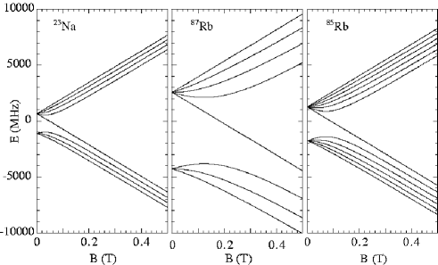
FIG. 3.: The Zeeman shifts for the ground state hyperfine states of (a) ²³Na, (b) ⁸⁷Rb and (c) ⁸⁵Rb. Note that the situations considered in this paper take place in a region located very close to $B=0$ in the scale of these pictures.

The necessary condition for evaporation is that the rf field induces a resonance between the states $M_{F}=2$ and $M_{F}=1$. The location of this resonance defines the division between the hot and cold atoms. By decreasing the rf field frequency $\nu_{\rm rf}$ we both move the resonance point closer to the trap center as well as allow more atoms to escape the trap. For small $B$ fields all adjacent states are resonant at the same location for any $\nu_{\rm rf}$. But in case of strong magnetic fields, typically larger than about 0.0002 T, due to the nonlinear Zeeman shifts the resonances separate. Furthermore, the other resonances than the $M_{F}=2-M_{F}=1$ one in fact move towards the trap center faster, and reach it while the $M_{F}=2-M_{F}=1$ resonance still corresponds to some finite temperature. When $\nu_{\rm rf}$ is lowered further, the other resonances begin to disappear. At strong $B$ fields the $M_{F}=0$ state is also a trapping state, as shown in Fig. 4, so for effective evaporation one really needs to reach the $M_{F}=-1$ state.

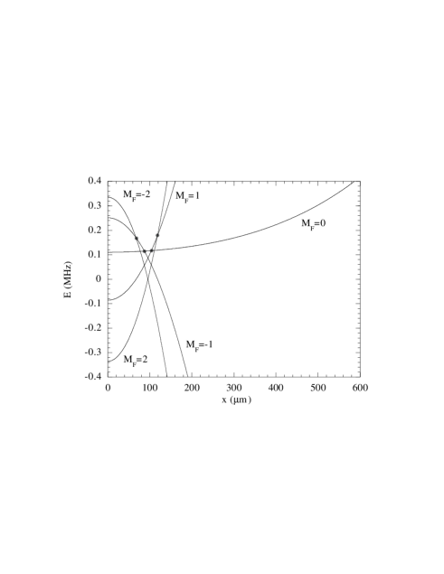
FIG. 4.: The $M_{F}=0$ state becomes a trapping state very quickly as $B$ increases. Here we show as an example the situation for ²³Na when $B_{0}=0.0010$ T. The oscillation frequency for this state is naturally much smaller than for the other trapping states.

At the critical frequency $\nu_{\rm cr}$ the crossing between the states $M_{F}=-1$ and $M_{F}=0$ disappears. Alternatively, for a fixed frequency $\nu_{\rm rf}$ we have a critical value $B_{\rm cr}$ for the $B$ field; the resonances disappear when $B\gtrsim B_{\rm cr}$ (for practical reasons we have chosen to modify $B$ rather than $\nu_{\rm rf}$ in our wave packet studies). In Fig. 5(a) we show the potential configuration when $\nu_{\rm rf}$ is slightly below $\nu_{\rm cr}$. Since $\nu_{\rm cr}$ corresponds to the state separation at the center of the trap, it is independent of the trap parameters such as the trap frequency.

For a specific trap configuration $\nu_{\rm cr}$ can be converted into a minimum kinetic energy required for reaching the resonance between the states $M_{F}=2$ and $M_{F}=1$. In Fig. 5(b) we show this minimum kinetic energy in units of temperature as a function of magnetic field strength for ²³Na and ⁸⁷Rb, and for the trap configuration used both in our simulations and in the experiment by Desruelle et al. [9].

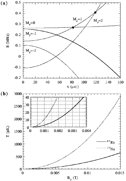
FIG. 5.: (a) For $B=0.00155$ T and $\nu_{\rm rf}=$0.25 MHz+$\nu_{0}$ the resonance between the $M_{F}=0$ and $M_{F}=-1$ states for ²³Na can not be achieved ($B_{\rm cr}=0.00152$ T). The possibility for a tunnelling-like transfer (which could also be called off-resonant process via power broadening) exists, though. (b) The lowest energy (in temperature units) for which evaporation is allowed as a function of trap center field $B_{0}$ for ⁸⁷Rb and ²³Na with the trap parameters used in this paper.

In the intermediate region $0\ll B\lesssim B_{\rm cr}$, where the necessary crossings exist but are separated, the processes take place via two possible routes. We can have off-resonant multiphoton processes, that e.g. lead to adiabatic transfer from the $M_{F}=2$ state to the $M_{F}=0$ state. This example is demonstrated in Fig. 2 where we show also the eigenstates of the system, i.e., the field-dressed potentials. When the relevant resonances are well separated, the evaporation takes place via a complicated sequence of crossings, as indicated in Fig. 1(c). This will be demonstrated with wave packet simulations in Sec. IV.

B ⁸⁵Rb

For the isotope ⁸⁵Rb we have $I=5/2$ and $J=1/2$, so the ground state hyperfine states are $F=2$ and $F=3$, as shown in Fig. 3(c). Now the $F=2$ trapping state is the lower hyperfine ground state. Thus the behavior of the $M_{F}$ states is different from the ⁸⁷Rb and ²³Na case. The $B$ field dependence of the states related to $F=2$ is now

$$E_{+2} = \frac{3A}{2}-\frac{1}{2}\sqrt{9A^{2}+4AC+C^{2}},$$ (8)

$$E_{+1} = \frac{3A}{2}-\frac{1}{2}\sqrt{9A^{2}+2AC+C^{2}},$$ (9)

$$E_{0} = \frac{3A}{2}-\frac{1}{2}\sqrt{9A^{2}+C^{2}},$$ (10)

$$E_{-1} = \frac{3A}{2}-\frac{1}{2}\sqrt{9A^{2}-2AC+C^{2}},$$ (11)

$$E_{-2} = \frac{3A}{2}-\frac{1}{2}\sqrt{9A^{2}-4AC+C^{2}},$$ (12)

where now $E_{\rm hf}=3A$. For ⁸⁵Rb we have $\nu_{\rm hf}$ = 3036 MHz. Here the trapping states are now $F=2,M=-2$ and $F=2,M=-1$. If we now define $\tilde{\varepsilon}=(2/3)\varepsilon=\mu_{B}B/(3E_{\rm hf})$ we get approximatively

$$E_{\rm M_{F}}\simeq-E_{\rm hf}[\tilde{\varepsilon}M_{F}+(9-M_{F}^{2})\tilde{\varepsilon}^{2}].$$ (13)

As $g_{F}=-1/3$, this agrees with the linear expression $E_{\rm M_{F}}=g_{F}\mu_{B}BM_{F}=-E_{\rm hf}\tilde{\varepsilon}M_{F}$.

FIG. 6.: The effect of nonlinear Zeeman shifts on the evaporation from the ⁸⁵Rb $F=2$ state. The circles indicate for which crossing points the couplings are nonzero. The numbers indicate the order in which an atom moving out of the trap traverses the crossings. The kinetic energy required to leave the trap is now determined by the difference between the trap center and the second crossing. Here $B_{0}=0.0050$ T and $\nu_{\rm rf}=$0.25 MHz+$\nu_{0}$, with $\nu_{0}=(E_{-2}-E_{-1})/h$.

The change of order in the $M_{F}$ state energy ladder means that with increasing $B$ field one never loses the crossing points between the adjacent states. In other words, if we use an rf field that can couple the states $M_{F}=-2$ and $M_{F}=-1$ resonantly at some location $x_{C}$, then we always couple the rest of the states resonantly as well at distances larger than $x_{C}$. In Fig. 6 we see how this leads to a sequence of crossings that allows hot atoms to leave the trap without the need for sloshing. One must, however, take into account that the kinetic energy required to leave the trap is now set by the difference between the energy of the $M_{F}=-2$ state at the center of the trap, and the energy of the $M=0$ (or $M_{F}=-1$) state at the point where the states $M_{F}=0$ and $M_{F}=-1$ are in resonance. In other words, atoms need a kinetic energy equal or larger to the energy difference between the trap center and the second crossing in Fig. 6.

In this paper we limit our discussion on the $F=2$ case only, but it is obvious that for the ⁸⁵Rb $F=3$ trapping states we face the same problem as in the $F=2$ case for ⁸⁷Rb and ²³Na. In general for the alkali atoms we can expect that the problem will arise whenever we use the upper ground state hyperfine state as the trapping state at strong $B$ fields.

C Trap configuration

For simplicity we have assumed in our studies the same spatially inhomogeneous magnetic field as in the experiment by Desruelle et al. [9], except that we have added a spatially homogeneous compensation field. This allows us to change the general field magnitude (depends on the bias field) while keeping the trap shape almost unchanged (depends also on the bias field). Thus we set [9]

$$B=B_{0}+\left(\frac{B^{\prime 2}}{2B_{\rm bias}}-\frac{B^{\prime\prime}}{2}\right)(x^{2}+y^{2})+B^{\prime\prime}z^{2},$$ (14)

where $B^{\prime}=9$ T/m, $B^{\prime\prime}/B_{\rm bias}=10^{4}$ m^-2, and the trap center field is defined as $B_{0}\equiv B_{\rm bias}-B_{\rm comp}$. The actual trap is cigar-shaped, which is a typical feature in many experiments. We have selected the $x$ direction as the basis for our wave packet studies. We set $B_{\rm bias}=0.0150$ T and use $B_{\rm comp}$ as a parameter to change $B_{0}$. Using $C=g_{J}\mu_{B}B$ with Eqs. (4) and (14) we get the spatially dependent trapping potentials.

III Quantum and semiclassical models

A Wave packet simulations

For our wave packet studies we fix the rf field frequency to the value $\nu_{\rm rf}=\nu_{0}+0.25$ MHz, where $\nu_{0}=[E_{+2}(x=0)-E_{+1}(x=0)]/h$. With this setting the atoms need typically a kinetic energy about $E_{\rm kin}/k_{B}\simeq 24\ \mu$K in order to reach the crossing between the states $M_{F}=2$ and $M_{F}=1$. With our special definition of $\nu_{\rm rf}$ the differences between ²³Na and ⁸⁷Rb appear mainly in the time scale of atomic motion (Na atoms are lighter and thus move faster), and in scaling of $B$. For our selected $\nu_{\rm rf}$ we have $B_{\rm cr}=0.00297$ T for ⁸⁷Rb and $B_{\rm cr}=0.00152$ T for ²³Na. We have used the rf field strength $\Omega=(2\pi)2.0$ kHz), where the rf field induced coupling term is [3, 8]

$${\cal H}=\hbar\left(\begin{array}[]{ccccc}0&\Omega&0&0&0\\ \Omega&0&\sqrt{\frac{3}{2}}\Omega&0&0\\ 0&\sqrt{\frac{3}{2}}\Omega&0&\sqrt{\frac{3}{2}}\Omega&0\\ 0&0&\sqrt{\frac{3}{2}}\Omega&0&\Omega\\ 0&0&0&\Omega&0\end{array}\right)\quad\begin{array}[]{l}|2,-2\rangle\\ |2,-1\rangle\\ |2,0\rangle\\ |2,1\rangle\\ |2,2\rangle\end{array},$$ (15)

in the $|F,M_{F}\rangle$ basis as indicated.

The wave packet simulations were performed in the same manner as in the previous study [3]. Our initial wave packet has a Gaussian shape, with a width of $10\ \mu$m. For all practical purposes this wave packet is very narrow both in position and momentum, and the spreading due to its natural dispersion is not an important factor. We identify the mean momentum of the wave packet with the atomic kinetic energy $E_{\rm kin}$, and set $E_{\rm kin}/k_{B}=30\ \mu$K. In the experiment by Desruelle et al. one had typically $B_{0}=B_{\rm bias}=0.0150$ T, which sets the kinetic energy for reaching the resonance points (for any practical value of $\nu_{\rm rf}$) too large for realistic numerical simulations. Thus we have introduced the compensation field and limit $B_{0}$ to values below $0.0050$ T. But the main conclusions from our study apply to larger values of $B_{0}$ and $E_{\rm kin}$, and many of the results can be scaled to other parameter regions with the semiclassical models.

Another simplification is that we consider only one spatial dimension. This is necessary simply because we have chosen to work with relatively large energies, such as 30 $\mu$K. Numerical wave packet calculations at the corresponding velocities require on the order of 100 000 points for both the spatial and temporal dimensions. As discussed in Ref. [3], however, this is not a crucial simplification.

Basically, we solve the five-component Schrödinger equation

$$i\hbar\frac{\partial\Psi(x,t)}{\partial t}={\cal H}(x)\Psi(x,t),$$ (16)

The components of the state vector $\Psi(x,t)$ stand for the time dependent probability distributions for each $M_{F}$ state. The off-diagonal part of the Hamiltonian ${\cal H}$ is given Eq. (15). The diagonal terms are

$$-\frac{\hbar^{2}}{2m}\frac{\partial^{2}}{\partial x^{2}}+U_{\rm M_{F}}(x)-M_{F}h\nu_{\rm rf},$$ (17)

where $m$ is the atomic mass and $U_{\rm M_{F}}(x)$ are the trap potentials as in Fig. 1(a). For states $M_{F}=-2$ and $M_{F}=-1$ we use absorbing boundaries, and reflecting ones for the others. The numerical solution method is the split operator method, with the kinetic term evaluated by the Crank-Nicholson approach [13, 14].

B Semiclassical models

For small magnetic fields the rf field induced resonances between adjacent states occur at the same position, $x=x_{C}$. In this situation the spin-change probability for atoms which traverse the resonance is given by the multistate extension [8, 15] of the two-state Landau-Zener model [16]. We have earlier shown that for the evaporation in ²³Na $F=2$ state at $E_{\rm kin}/k_{B}=5\ \mu$K and small $B$ this model predicts the wave packet results very well [3].

The solution for the multistate problem can be expressed with the solutions to the two-state Landau-Zener (LZ) model, so we shall begin by discussing the two-state case first. Let us consider two potentials, $U_{1}$ and $U_{2}$, which intersect at $x=x_{C}$ and are coupled by $V$. For strong $B$, when the crossings are well separated in our alkali $F=2$ system, $V$ is equal to $\hbar\Omega$ or $\sqrt{3/2}\hbar\Omega$, depending which pair of adjacent states is involved [see Eq. (15)].

In addition to the coupling $V$, the relevant factors are the speed $v_{C}$ of the wave packet and the slopes of the trapping potentials $U_{\rm M_{F}}(x)$ at the crossing. We define

$$\alpha=\hbar\left|\frac{d(U_{2}-U_{1})}{dx}\right|_{x=x_{C}}.$$ (18)

The speed of the wave packet enters the problem as we describe the traversing of the crossing with a simple classical trajectory, $x=v_{C}(t-t_{0})+x_{0}$. This allows us to enter the purely time-dependent description where the population transfer is given by the two-component Schrödinger equation

$$i\hbar\frac{\partial}{\partial t}\left(\begin{array}[]{c}\Psi_{1}(t)\\ \Psi_{2}(t)\end{array}\right)=\left(\begin{array}[]{cc}0&V\\ V&\alpha v_{C}t\end{array}\right)\left(\begin{array}[]{c}\Psi_{1}(t)\\ \Psi_{2}(t)\end{array}\right).$$ (19)

This is the original Landau-Zener theory. In this form it is fully quantum and we can obtain an analytic expression for state populations $P_{1}$ and $P_{2}$ after the crossing. If state 1 was the initial state, then

$$\begin{array}[]{ll}P_{1}&=1-\exp(-\pi\Lambda)\\ P_{2}&=\exp(-\pi\Lambda)\end{array},\qquad\Lambda=\frac{2V^{2}}{\hbar\alpha v_{C}}.$$ (20)

Obviously, the Landau-Zener model is only applicable when the total energy is higher than the bare-state energy at the resonance point. For more details about applying LZ theory to wave packet dynamics see Refs. [14, 17, 18].

And now we return to the original multistate problem. According to the five-state case of the multistate model (see e.g. Ref. [8]) the populations $P_{\rm M_{F}}$ for the untrapped states after one traversal of the crossing are

$$P_{2} = p^{4},$$ (21)

$$P_{1} = 4(1-p)p^{3},$$ (22)

$$P_{0} = 6(1-p)^{2}p^{2},$$ (23)

$$P_{-1} = 4(1-p)^{3}p,$$ (24)

$$P_{-2} = (1-p)^{4},$$ (25)

where $p=\exp(-\pi\Lambda)$, and $\Lambda$ is defined by setting $V=\hbar\Omega/2$. This assumes that we were intially on state $M_{F}=2$. We can see that the final population of the initial state, $P_{2}$, is equal to $\exp[-\pi\hbar\Omega^{2}/(2\alpha v_{C})]$ for both the two-state and the multistate model if Hamiltonian (15) is used.

IV Results

Typical examples of the atomic wave packet evolution for the three trapping states are shown in Figs. 7 and 8. They demonstrate the sloshing discussed e.g. in Refs. [3, 6, 9]. The amplitudes of the components decrease as population is partly transferred to another state. Similarly new wave packet components can appear at crossings. As a wave packet component reaches a turning point it sharpens strongly. In Fig. 7 we have $B_{0}=0.0018$ T, which means that there is no crossing between states $M_{F}=0$ and $M_{F}=-1$. Population transfer from the state $M_{F}=1$ to $M_{F}=0$ is weak. The $M_{F}=0$ wave packet component has turning points beyond the integration space.

As sloshing continues Stückelberg oscillations could take place as split wave packet components merge again at crossings and interfere (for further discussion, see Refs. [14, 19]). However, the wave packet contains several momentum components and thus such oscillations are not likely observed, because they are very sensitive to phase differences. In our simulations we saw no major indication of inteferences.

In Fig. 9 we track the trap state populations and their sum as the wave packet sloshes in the trap and traverses several crossings. The magnetic field values are strong enough to ensure that the crossings are well separated. We can identify when the various crossings take place although some of them happen simultaneously. The filled symbols indicate the corresponding Landau-Zener predictions, and we find that the agreement is excellent. Some oscillations appear for the ²³Na case [Fig. 7(a)] at times between 3.5 ms and 4.5 ms. These may arise from Stückelberg oscillations, but they do not affect the final transition probabilities, supporting our assumption that in the end such oscillations average out. Note that for ²³Na there is no resonance between states $M_{F}=0$ and $M_{F}=-1$, but for ⁸⁷Rb there is and it is seen as a stepwise reduction of $P_{S}\equiv P(M_{F}=2)+P(M_{F}=1)+P(M_{F}=0)$.

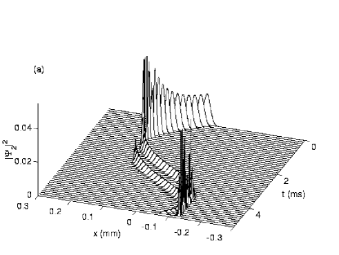
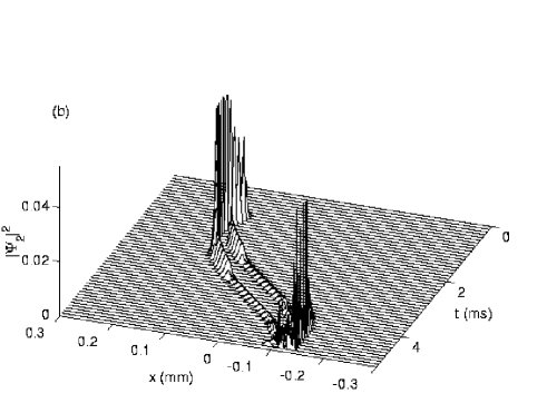
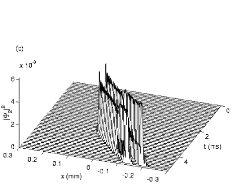
FIG. 7.: The evolution of the wave packet components $|\Psi_{\rm M_{F}}(x,t)|^{2}$ for ²³Na at $B_{0}=0.0018$ T and $\Omega=(2\pi)2$ kHz. (a) $M_{F}=2$, (b) $M_{F}=1$, and (c) $M_{F}=0$.

Near the critical field $B_{\rm cr}$ the probability to leave the trap via states $M_{F}=-2$ and $M_{F}=-1$ varies strongly with $B_{0}$. When $B_{0}<B_{\rm cr}$ the wave packet meets two crossings between the states $M_{F}=-1$ and $M_{F}=0$ as it traverses the region around the trap center $x=0$ on state $M_{F}=0$. At both crossings some population leaks into the state $M_{F}=-1$, as seen in Fig. 10 for $B_{0}=0.0028$ T. As $B_{0}$ increases, the two crossing points, on opposite sides of $x=0$, begin to merge, until they disappear at $x=0$ when $B=B_{\rm cr}$. Then the transfer between the two states becomes off-resonant (or tunnelling), and its probability decreases exponentially as a function of some ratio of $\Omega$ and the energy difference between the states $M_{F}=-1$ and $M_{F}=0$ at $x=0$. This situation corresponds to the parabolic level crossing model [20]. But the main point is that the off-resonant process is unlikely to play any major role.

Finally, in Fig. 11 we show how the transfer probability between the trap states at the first crossing changes as a function of $B_{0}$. The multistate process transforms smoothly into a two-state process between the states $M_{F}=2$ and $M_{F}=1$. The transition zone is rather large, though, with $B_{0}$ ranging from 0 to 0.0010 T. The transfer process in this zone is the off-resonant two-photon transfer demonstrated in Fig. 2. An analogous process can occur in atoms interacting with chirped pulses [21].

An interesting point is that the population of the initial state is not affected by the fact how the transferred population is distributed to the other involved states. This seems to be typical for the Landau-Zener crossings [22]. The solid lines indicate the predictions of the two-state model, and the dotted lines the multistate model. They change with $B_{0}$ because the location of the first crossing point and thus the wave packet speed $v_{C}$ at this point change slightly with $B_{0}$.

V Conclusions

Our results show that in general the semiclassical level crossing models offer a clear understanding of the single atomic dynamics during the evaporation process. Also, we have verified with wave packet calculations that the interpretations presented by Desruelle et al. for their ⁸⁷Rb experiment [9] are correct. The simple picture of evaporation at near-zero magnetic fields transforms into a complex sequence of two-state crossings at field strengths above about 0.0010 T. For all alkali systems where $F=2$ is the upper hyperfine ground state the evaporation will stop before condensation as the necessary resonances disappear too soon as a function of the rf field frequency. We have shown that tunnelling does not really play a role once the resonances have been lost. Further complications arise from the fact that the $M_{F}=0$ state becomes a trapping state.

In experiments, as suggested by Desruelle et al., one could avoid the problem by coupling the $F=2,M_{F}=2$ trapping state to the $F=1,M_{F}=1$ nontrapping state, or by using several rf fields of different frequencies within the $F=2$ hyperfine manifold. Although for ⁸⁷Rb one has observed a long-lasting coexistence of $F=1$ and $F=2$ condensates, theoretical studies [23] predict this difficult for ²³Na due to destructive collisions. Thus the first approach may apply better for ⁸⁷Rb than for ²³Na.

We have calculated earlier [3] that for ²³Na the collisions between atoms in the $M_{F}=0$ and $M_{F}=2$ states are very destructive, with a rate coefficient on the order of $10^{-11}$ cm³/s. For practical bias field strengths the $M_{F}$ state is also a trapping state. Thus the efficiency of evaporation is reduced, and the time the atoms spend on the $M_{F}=0$ state increase, making it more likely to have a destructive, energy releasing collision. So far condensation on the $F=2$ state for Na has not been achieved. Even in the weak $B$ field case evaporation can produce atoms on $M_{F}=0$ state via nonadiabatic transitions. Thus the role of inelastic collisions is expected to be enhanced for the field strengths considered here.

Once condensation is reached, however, the nonlinearity of the Zeeman shifts can be an asset rather than a nuisance. For instance, one could create a new type of binary condensates by making a selective transfer of part of the condensate from the $F=2,M_{F}=2$ state to the $F=2,M_{F}=1$ state, either by using resonant or chirped rf field pulses. Alternatively, two rf pulses of different frequencies or perhaps a single chirped pulse might allow one to transfer the condenstate from the $F=2,M_{F}=2$ state to the $F=2,M_{F}=0$ state and let it expand normally, without the need to switch the magnetic fields off. Of course, this would work only when $B$ is so small that the trapping nature of the $M_{F}$ state is not too strong.

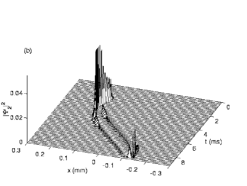
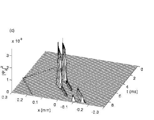
FIG. 8.: The evolution of the wave packet components $|\Psi_{\rm M_{F}}(x,t)|^{2}$ for ⁸⁷Rb at $B_{0}=0.0028$ T and $\Omega=(2\pi)2$ kHz. (a) $M_{F}=2$, (b) $M_{F}=1$, and (c) $M_{F}=0$.

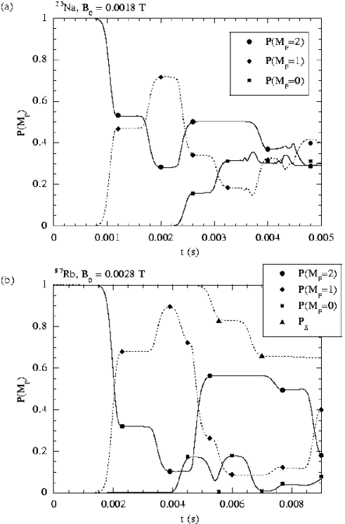
FIG. 9.: The time evolution of the trap state populations.

FIG. 10.: The time evolution of the trapped population for ⁸⁷Rb near the critical field strength $B_{\rm cr}$.

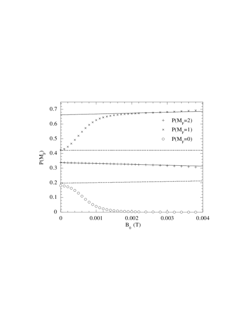
FIG. 11.: The population transfer after the first crossing for ⁸⁷Rb as a function of $B_{0}$. The solid lines are the semiclassical two-state predictions, and the dotted ones are the multistate model predictions. The symbols represent the wave packet results.

- [1] M. H. Anderson, J. R. Ensher, M. R. Matthews, C. E. Wieman, and E. A. Cornell, Science 269, 198 (1995); C. C. Bradley, C. A. Sackett, J. J. Tollett, and R. G. Hulet, Phys. Rev. Lett. 75, 1687 (1995); K. B. Davis, M.-O. Mewes, M. R. Andrews, N. J. van Druten, D. S. Durfee, D. M. Kurn, and W. Ketterle, Phys. Rev. Lett. 75, 3969 (1995).
- [2] C. J. Myatt, E. A. Burt, R. W. Ghrist, E. A. Cornell, and C. E. Wieman, Phys. Rev. Lett. 78, 586 (1997).
- [3] K.-A. Suominen, E. Tiesinga, and P. S. Julienne, Phys. Rev. A 58, 3983 (1998).
- [4] H. F. Hess, Phys. Rev. A 34, 3476 (1986).
- [5] T. Tommila, Europhys. Lett. 2, 789 (1986).
- [6] W. Ketterle and N. J. van Druten, Adv. At. Mol. Opt. Phys. 37, 181 (1996).
- [7] D. E. Pritchard, K. Helmerson, and A. G. Martin, At. Phys. 11, 179 (1988).
- [8] N. V. Vitanov and K.-A. Suominen, Phys. Rev. A 56, R4377 (1997).
- [9] B. Desruelle, V. Boyer, S. G. Murdoch, G. Delannoy, P. Bouyer, A. Aspect, and M. Lécrivain, Phys. Rev. A 60, R1759 (1999).
- [10] B. H. Bransden and C. J. Joachain, Physics of atoms and molecules (Addison-Wesley, Harlow, 1983).
- [11] M. E. Rose, Elementary theory of angular momentum (Dover, New York, 1995).
- [12] C. J. Pethick and H. Smith, Bose-Einstein condensation in dilute gases (HCØTryk, Copenhagen, 1997).
- [13] K.-A. Suominen, B. M. Garraway, and S. Stenholm, Phys. Rev. A 45, 3060 (1992).
- [14] B. M. Garraway and K.-A. Suominen, Rep. Prog. Phys. 58, 365 (1995).
- [15] A. K. Kazansky and V. N. Ostrovsky, J. Phys. B 29, L855 (1996); V. N. Ostrovsky and H. Nakamura, J. Phys. A 30, 6939 (1997).
- [16] C. Zener, Proc. R. Soc. Lond. Ser. A 137, 696 (1932); K.-A. Suominen, B. M. Garraway, and S. Stenholm, Opt. Commun. 82, 260 (1991); N. V. Vitanov and B. M. Garraway, Phys. Rev. A 53, 4288 (1996).
- [17] K.-A. Suominen and B. M. Garraway, Phys. Rev. A 48, 3811 (1993).
- [18] K.-A. Suominen, M. J. Holland, K. Burnett, and P. S. Julienne, Phys. Rev. A 49, 3897 (1994); K.-A. Suominen, J. Phys. B 29, 5981 (1996).
- [19] B. M. Garraway and S. Stenholm, Phys. Rev. A 46, 1413 (1992).
- [20] K.-A. Suominen, Opt. Commun. 93, 126 (1992).
- [21] D. J. Maas, C. W. Rella, P. Antoine, E. S. Toma, and L. D. Noordam, Phys. Rev. A 59, 1374 (1999).
- [22] V. M. Akulin and W. Schleich, Phys. Rev. A 46, 4110 (1992).
- [23] P. S. Julienne, F. H. Mies, E. Tiesinga, and C. J. Williams, Phys. Rev. Lett. 78, 1880 (1997).