Analyzing symmetry breaking within a chaotic quantum system via Bayesian inference

Abstract

Bayesian inference is applied to the level fluctuations of two coupled microwave billiards in order to extract the coupling strength. The coupled resonators provide a model of a chaotic quantum system containing two coupled symmetry classes of levels. The number variance is used to quantify the level fluctuations as a function of the coupling and to construct the conditional probability distribution of the data. The prior distribution of the coupling parameter is obtained from an invariance argument on the entropy of the posterior distribution.

I Introduction

The subject of the present paper is Bayesian inference as applied to the experiment of Ref. [1] in order to extract the mean square matrix element coupling two chaotic classes of quantum states. The Bayesian procedure described below does not contain any arbitrary element: The prior distribution — sometimes left to the educated guess of the analyst [2] — is determined by an invariance argument on the entropy of the posterior distribution.

The present article is organized as follows. In Sec. II, we briefly describe the experiment with superconducting microwave resonators that has provided the data for the present analysis. The random matrix model for the coupling of two symmetry classes of chaotic states is defined in Sec. III. It yields — in analytic form — the dependence of the observable on the coupling strength which is to be determined. Bayesian inference, especially the definition of the prior distribution, is discussed in Sec. IV. The conditional probability distribution of the data is defined in Sec. V. The results are given in Sec. VI. A discussion in Sec. VII concludes the paper.

II The experiment with coupled microwave resonators

Billiards provide models of classical and quantum mechanical chaos. They have been studied extensively, see the review article [3]. Quantum mechanical billiards can be simulated by flat microwave resonators [4, 5, 6, 7]. One class of these “quantum” billiards are the Bunimovich stadium billiards [8] experimentally investigated in Refs. [1, 7, 9, 10, 11, 12].

These investigations show that the fluctuation properties of the quantum chaotic systems with well defined symmetries are described by Dyson’s matrix ensembles [3]. In the case of the stadium billiards, the correct description is provided by the Gaussian Orthogonal Ensemble (GOE). This means, e.g., that the fluctuations of the positions of the eigenmodes — shortly the level fluctuations — are the same as the fluctuations of the eigenvalues of random matrices drawn from the GOE. In order to assess these fluctuations, various statistics have been defined — such as the distance of neighboring levels or the variance of the number of levels in a given interval. The expectation values of these statistics have been worked out [13, 14] for comparison with data such as the present ones.

In the previous work [1], the level positions of a system have been measured that consisted of two (quarters of) stadium billiards coupled electromagnetically. See Fig. 1. The technical realization of the coupling has been described in Ref. [1]. In the frequency range of 0 to 16 GHz, the complete spectra of the two stadia displayed 608 and 883 resonances in the $(\gamma=1)$ stadium and the $(\gamma=1.8)$ stadium, respectively. The mean level spacing is $D=10.7$ MHz.

In Fig. 2, small pieces of spectra are shown for three different couplings. The arrows shall help to recognize that — due to the coupling — the resonances are shifted by statistically varying amounts.

This system simulates two symmetry classes of levels coupled by a symmetry breaking interaction. Each class of levels — represented by each of the uncoupled stadia — can be identified with a chaotic system of well defined symmetry having the properties of the GOE. The entire system of the coupled stadia no longer has the universal properties of the GOE. Its properties are a function of a suitably defined coupling parameter $\Lambda$.

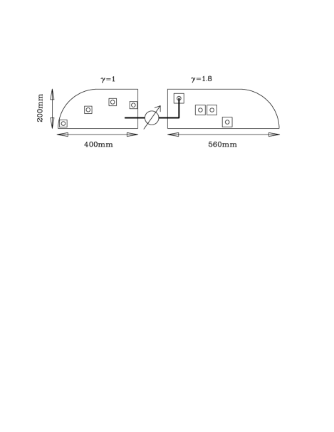
FIG. 1.: Shapes of the two coupled stadium billiards. The circles inside the squares indicate the positions of the antennas used to scatter microwave power through the system in order to find the eigenfrequencies of the entire system. The parameter $\gamma$ is the ratio between the length of the rectangular part and the radius of the circular part of the resonator. The vertical heights of the stadia are given in Sec. VI.

FIG. 2.: Three spectra — within a small range of frequencies — taken at different couplings between the two resonators. The coupling increases from top to bottom. Its notation $(x,y)$ is explained in Sec. VI. The arrows shall help to recognize the shifts of a few resonances.

The investigation of symmetry breaking in chaotic quantum systems is not a recent challenge to physicists [15]. Good examples of the experimental and theoretical efforts already invested into this problem, are the cases of isospin mixing [16, 17, 18], of parity violation in heavy nuclei [19], of the breaking of certain atomic and molecular symmetries [15, 20]. The experiment performed in [1] provides a general model for these case studies.

In the present paper, we do not describe any one of the specific case studies; we shall not even describe in more detail the model experiment of Ref. [1]. We rather describe — in the next section — the model experiment [1] in an abstract mathematical form and then turn to its analysis in Secs. IV-VII.

III The mathematical model of symmetry breaking in a chaotic quantum system

In the absence of coupling each eigenstate of the system of Fig. 1 can be characterized as belonging to either resonator 1 or resonator 2. This is equivalent to the assignment of a quantum number $\gamma$. The spectrum of states of each $\gamma$ has the statistical properties of the eigenvalues of matrices drawn from the GOE. The superposition of the two spectra displays what we shall call 2 GOE behavior. It can be described by a block-diagonal Hamilton operator where each block is an element of the GOE, hence, by the first term of the Hamiltonian

$${\cal H}=\left(\begin{array}[]{cc}\framebox[25.6073pt]{\rule[-1.42262pt]{0.0pt}{2.84544pt}$\mbox{GOE}$}&0\\ 0&\framebox[25.6073pt]{\rule[-1.42262pt]{0.0pt}{2.84544pt}$\mbox{GOE}$}\end{array}\right)+\alpha\left(\begin{array}[]{cc}\framebox[14.22636pt]{\rule[-0.28453pt]{0.0pt}{2.84544pt}0}&V\\ V^{+}&\framebox[14.22636pt]{\rule[-0.28453pt]{0.0pt}{2.84544pt}0}\end{array}\right).$$ (5)

For $\alpha\neq 0$, the off-diagonal matrix $V$ in the second term on the r.h.s. provides the coupling between both symmetry classes. It has Gaussian random elements — as the GOE blocks. If the two GOE blocks have the same dimension then their elements as well as the elements of $V$ shall all have the same rms value. Then $\alpha=1$ turns ${\cal{H}}$ as a whole into a GOE matrix [21]. The resulting spectrum displays what we call 1 GOE behavior. If the two GOE blocks have different dimensions, then the rms values must be chosen such that their spectra have the same length. The details are given in [14]. This model is a special case of the model by Rosenzweig and Porter [15].

The parameter that governs the level statistics is $\alpha v/D$ rather than $\alpha$. Here, $D$ is the mean level distance of $\cal H$. See Refs. [14, 18]. In the sequel, the coupling parameter

$$\Lambda=\left(\frac{\alpha v}{D}\right)^{2}$$ (6)

will be used. Often the coupling strength is also parametrized in terms of the spreading width

$$\Gamma^{\downarrow} = 2\pi\,\frac{(\alpha v)^{2}}{D}$$ (7)

$$= 2\pi\,\Lambda D.$$ (8)

The statistic used in the present paper in order to characterize the behavior of the data, is the so-called $\Sigma^{2}$ statistic or number variance. It is the variance $z(L)$ of the number $n(L)$ of levels found in an interval of length $LD$, i.e.

$$z(L)=\langle(n(L)-L)^{2}\rangle.$$ (9)

Here, the angular brackets $\langle\rangle$ denote the average over all pieces of spectra of length $L$ that have been cut out of the entire experimental spectrum. The procedure is described in Sec. V.

The expectation value $\overline{z(L)}$ with respect to the statistical ensemble defined by Eq. (5) is called $\Sigma^{2}(L,\Lambda)$. This function has been calculated by French et al. [13] and by Leitner et al. [14]. According to [14], it is

$$\Sigma^{2}(L,\Lambda) = \overline{z(L)}$$ (10)

$$= \Sigma^{2}(L,\infty)+\frac{1}{\pi^{2}}\ln\left(1+\frac{\pi^{2}L^{2}}{4(\tau+\pi^{2}\Lambda)^{2}}\right).$$ (11)

Here, $\Sigma^{2}(L,\infty)$ is the expression

$$\Sigma^{2}(L,\infty) = \frac{2}{\pi^{2}}\left\{\ln(2\pi L)+\gamma_{E}+1+\frac{1}{2}\left[{\mbox{Si}}(\pi L)\right]^{2}\right.$$ (14)

$$-\frac{\pi}{2}{\mbox{Si}}(\pi L)-\cos(2\pi L)-{\mbox{Ci}}(2\pi L)$$

$$+\left.\pi^{2}L\left[1-\frac{2}{\pi}{\mbox{Si}}(2\pi L)\right]\right\}.$$

It describes the 1 GOE behavior. The second term on the r.h.s. of Eq. (11) obviously vanishes for $\Lambda\rightarrow\infty$.

In Eq. (14), $\gamma_{E}$ is Euler’s constant and Si, Ci are the sine and cosine integrals defined e.g. in paragraph 8.23 of [22]. The parameter $\tau$ is a function of the ratio between the dimensions of the two GOE blocks in the first term of Eq. (5). In the present situation, it is equal to 0.74.

The function $\Sigma^{2}$ depends on the coupling parameter $\Lambda$ — as is illustrated by Fig. 3. Therefore $\Lambda$ can be inferred from the experimental number variance $z(L)$ . The principle of this inference is described in the next section.

FIG. 3.: The expectation value $\Sigma^{2}(L,\Lambda)$ of the number variance $z(L)$ as a function of $L$ for various coupling strengths $\Lambda$ — ranging from 2 GOE to 1 GOE behavior. The abscissa has been limited to $L\leq 5$ because the data analyzed below are in the range of $1\leq L\leq 5$.

IV Bayesian inference

Suppose that a set of experimental data $z_{k}$, $k=1...M$, is given which depends on a parameter $\Lambda$ in the sense that the probability distribution $w_{k}$ of the event $z_{k}$ is conditioned by the hypothesis $\Lambda$,

$$w_{k}=w_{k}(z_{k}\mid\Lambda).$$ (15)

The events $z_{k}$ shall be statistically independent of each other. The joint distribution $W$ of the $z_{k}$, $k=1...M$, is then

$$W(z\mid\Lambda)=\displaystyle\prod^{M}_{k=1}w_{k}(z_{k}\mid\Lambda).$$ (16)

From this follows the distribution $P(\Lambda\mid z)$ of $\Lambda$ under the condition that the data $z$ are given via Bayes’ theorem

$$P(\Lambda\mid z)=\frac{W(z\mid\Lambda)\,\mu(\Lambda)}{m(z)}.$$ (17)

Here, $\mu(\Lambda)$ is the so-called prior distribution. It is the measure of integration in the space of $\Lambda$. One must define it such that it represents ignorance on $\Lambda$ — in a sense described below. The function $m(z)$ is the prior distribution of $z$. It is not independent of $\mu$; it is given by the normalizing integral

$$m(z)=\int d\Lambda\,\,W(z\mid\Lambda)\,\mu(\Lambda).$$ (18)

In the framework of the logic underlying Eq. (17), a probability distribution of — say — $\Lambda$ is considered to represent the available knowledge on $\Lambda$ and the prior distribution corresponds to “ignorance about $\Lambda$”.

The definition of $\mu(\Lambda)$ deserves a detailed comment. First of all, the natural choice of $\mu(\Lambda)$ is not the constant function because a reparametrization $\Lambda\rightarrow\lambda(\Lambda)$ will transform $\mu(\Lambda)$ into

$$\displaystyle\mu_{T}(\lambda)=\mu(\Lambda)\left|\frac{d\Lambda}{d\lambda}\right|.$$ (19)

Unless the transformation is linear, it turns a uniform distribution into a non-uniform one.

We define $\mu(\Lambda)$ such that the entropy of $P(\Lambda|z)$ does not depend on the true value $\hat{\Lambda}$ that governs the distribution of the data $z=(z_{1}...z_{M})$. The data follow the distribution $W(z|\hat{\Lambda})$. Although $\hat{\Lambda}$ is not known, it is supposed to be a well defined number. If it is shifted to another value $\hat{\Lambda}^{\prime}$ and one takes new data $z^{\prime}$ and constructs the posterior distribution $P^{\prime}=P(\Lambda|z^{\prime})$ from the new data, then one can expect $P^{\prime}$ to be shifted with respect to $P$. The distribution $P^{\prime}$ will be centered in the vicinity of $\hat{\Lambda}^{\prime}$ rather than $\hat{\Lambda}$. However, we want to make sure that the “spread” of $P^{\prime}$ is the same as that of $P$; that is, the entropy of $P$ and $P^{\prime}$ shall be the same — for a given number of data $M$. In this sense, no value of $\Lambda$ is a priori preferred over any other one.

The definition of the entropy requires some attention. The usual formula $-\int d\Lambda\,P\ln\,P$ for the entropy is of too restricted validity in the present context, because this expression is not invariant under a reparametrization $\Lambda\rightarrow\lambda(\Lambda)$. The general expression for the entropy is

$$\displaystyle H=-\int d\Lambda\,P(\Lambda|z)\,\ln\frac{P(\Lambda|z)}{\mu(\Lambda)}$$ (20)

which is independent of a reparametrization [23, 24], because the transformations of both distributions, $P$ and $\mu$, are performed according to (19). Therefore the derivative $|d\Lambda/d\lambda|$ drops out of the argument of the logarithm and expression (20) is left unchanged by the substitution $\Lambda\rightarrow\lambda$.

It is possible to define $\mu$ such that $H$ is independent of the true value $\hat{\Lambda}$, if $W$ possesses the property introduced in [24, 25, 26] called form invariance. It states that there is a group of transformations $\cal{G}_{\rho}$ such that the simultaneous transformation of $z$ and $\Lambda$ leaves $W$ invariant, i.e.

$$\displaystyle W({\cal{G}}_{\rho}z|{\cal{G}}_{\rho}\Lambda)\,d{\cal{G}}_{\rho}z=W(z|\Lambda)\,dz.$$ (21)

The group parameter $\rho$ must have the same domain of definition as the hypothesis $\Lambda$. If one chooses $\mu(\Lambda)$ to be the invariant measure of the group then it is not difficult to show that the posterior distribution $P$ also possesses the invariance (21). This entails that $H$ is invariant under any transformation $z\rightarrow{\cal{G}}_{\rho}z$ of the data. However, by Eq. (21) this is just what happens to a given data set if the true value $\hat{\Lambda}$ is shifted to $\hat{\Lambda}^{\prime}={\cal{G}}_{\rho}^{-1}\hat{\Lambda}$.

There is a handy formula that yields the invariant measure without any study of the structure of the group. It is

$$\displaystyle\mu(\Lambda)=\left|M^{-1}\int d^{M}z\,W(z\mid\Lambda)\frac{\partial^{2}}{\partial\Lambda^{2}}\ln W(z\mid\Lambda)\right|^{1/2}$$ (22)

and was proposed by Jeffreys [27] even before form invariance was discussed.

Not every conditional distribution $W$ possesses a symmetry (21). Even if this is not the case, expression (22) ensures that $H$ is approximately independent of the true value of $\Lambda$. This holds in the following sense: For every $\hat{\Lambda}$ one can replace the correct distribution $W(z\mid\Lambda)$ by an approximation $W_{app}(z\mid\Lambda)$ which is form invariant. The approximate and the correct distributions agree within the fourth order of $\Lambda-\hat{\Lambda}$. Equation (22) yields the invariant measure of the approximation to within the third order of $\Lambda-\hat{\Lambda}$ [28].

In summary: expression (22) ensures that no value of $\Lambda$ is a priori preferred over any other one if the form invariance (21) exists. If there is no form invariance, expression (22) approximately ensures this. Therefore (22) is the best recommendation in any case.

Neither the group theoretic argument nor Jeffreys’ rule nor information theoretic arguments are new in the discussion of the Bayesian prior. However, the way in which they are related justifies the present digression on a fundamental issue. We omit to show how and why the present arguments are related to the geometric considerations which were introduced by Amari [29] and are currently put forward by Rodriguez [30]. These authors agree on the result (22).

The posterior distribution $P$ is used to construct an interval of error often called a confidence interval. It is the shortest interval that contains $\Lambda$ with probability $K$. The usual error is defined with the confidence $K=0.68$.

The posterior distribution $P$ approaches a Gaussian for $M\rightarrow\infty$ provided that the true value of $\Lambda$ is not on the border of the domain of definition of $\Lambda$. One can prove that the variance of the Gaussian is proportional to $M^{-1}$. Hence, with increasing $M$ the posterior distribution $P$ will become so narrow that $\mu$ changes very little in the domain where $P$ is essentially different from zero. Note that $\mu$ does not depend on $M$. Then $\mu$ drops out of expression (17). If this happens, the present Bayesian analysis becomes equivalent to a $\chi^{2}$ fit of $\Sigma^{2}(L,\Lambda)$ to the experimental points $z(L)$. The standard procedure of the $\chi^{2}$ fit can e.g. be found in [31]. It does not require a prior distribution.

If $P$ is not Gaussian, the $\chi^{2}$ fit yields meaningless confidence intervals. Then Bayesian inference cannot be bypassed. In the example presented below this happens in the limit of small coupling between the resonators: Eventually, the posterior distribution $P$ decreases monotonically. The experiment is then compatible with zero coupling because the shortest confidence interval contains the point $\Lambda=0$ for any $K$. The point of zero coupling is on the border of the domain of definition of $\Lambda$.

V The distribution of the data

Spectral fluctuation properties can only be studied after secular variations of the level density have been removed, i.e. after the frequency scale has been transformed such that the level density becomes unity within the interval covered by the experiment. This procedure — often called “unfolding” the spectrum — is a standard one [32] and has been applied.

After this we defined — for a given interval of length $L$ — $N_{L}$ adjacent intervals. The intervals did not overlap and no space was left in between them. This means

$$N_{L}=\left[\frac{{\mbox{length of spectrum}}}{L}\right],$$ (23)

where the square brackets designate the largest integer contained in the fraction. For each interval, the number $n(L)$ of levels occuring within it was counted and the squared difference $(n(L)-L)^{2}$ was averaged over the $N_{L}$ intervals. This defines the average $\langle\rangle$ introduced in Eq. (9) and, hence, the “event” $z(L)$. This procedure was repeated for a set of values $L_{k}$, $k=1...M$, to be defined below. In this way, $M$ events

$$z_{k}\equiv z(L_{k})$$ (24)

were obtained.

The Bayesian procedure outlined in the previous section requires that one assigns a probability distribution $w_{k}(z_{k}\mid\Lambda)$ to each event. The $z_{k}$ are statistical quantities in the following sense: If another spectrum would be provided that had the same statistical properties as the measured one and the data $z_{k}$ would be constructed in the same way as above, they would of course not coincide with the data obtained from the actually measured spectrum — precisely because the levels are subject to statistical fluctuations. If one could go through the ensemble of spectra in this way, one would obtain an ensemble of data $z_{k}$. We are looking for the distribution $w_{k}$ of this ensemble. Since there is only the single measured spectrum and since no theory yielding $w_{k}$ is available, we have generated the distribution of $z_{k}$ by Efron’s bootstrap method [33]. This method generates the distribution numerically by drawing at random and independently a new set of $N_{L_{k}}$ intervals from the $N_{L_{k}}$ original intervals. A new $z_{k}$ is produced from this new set of intervals. Repeating this many times, a distribution of $z_{k}$ is generated which is identified with the distribution $w_{k}$ of the $z_{k}$. Note that $N_{L_{k}}$ is always large, namely $N_{L_{k}}\gtrsim 300$.

For $L_{k}\geq 1$, the distribution $w_{k}$ was in this way found to be a $\chi^{2}$ distribution with $N_{L_{k}}$ degrees of freedom — which intuitively seems reasonable. They are close to Gaussians with variance $2/N_{L_{k}}$ As mentioned above in Sec. III, the mean value of this distribution is

$$\displaystyle\overline{z_{k}} = \int dz\,\,z\,w_{k}(z\mid\Lambda)$$ (25)

$$= \Sigma^{2}(L_{k},\Lambda).$$ (26)

Since $\Sigma^{2}$ depends on $\Lambda$ — see Eq. (11) — the distribution $w_{k}$ depends on $\Lambda$.

We have restricted the analysis to $L_{k}\geq 1$. In the domain of $L_{k}<1$, the number variance so weakly depends on the parameter $\Lambda$ that one does not give away much information by this restriction.

In order to avoid an unnecessarily complicated distribution of the $z_{k}$, we want to be sure that there are no correlations between $z_{k}$ and $z_{k^{\prime}}$, for $k\neq k^{\prime}$. It was therefore necessary to determine the minimum $\epsilon$ of the distance $\mid L_{k}-L_{k^{\prime}}\mid$ that would still allow for statistically independent $z_{k}$, $z_{k^{\prime}}$. Indeed if $\mid L_{k}-L_{k^{\prime}}\mid$ is very small then most of the intervals associated with $L_{k}$ will almost coincide with an interval associated with $L_{k^{\prime}}$. As a consequence, many of the numbers $n(L_{k})$ found in the intervals associated with $L_{k}$ will occur also in the intervals associated with $L_{k^{\prime}}$. Hence, $z_{k}$ will not be independent from $z_{k^{\prime}}$. In order to determine $\epsilon$, we have calculated $z(L)$ as a function of $L$ in steps of 0.001. For a small range of $L$, the result is given in Fig. 4. Indeed over a distance of a few times this step width, $z(L)$ changes little. If $\mid L-L^{\prime}\mid$ is many times this step width, then $z(L)$ and $z(L^{\prime})$ show independent fluctuations. In principle, one can study the decay of the correlations as a function of $\mid L-L^{\prime}\mid$ by constructing the autocorrelation function of $z(L)$. We have contented ourselves to inspect Fig. 4 and similar plots for different domains of $L$. It seems obvious from Fig. 4 that the typical width of the structures is less than 0.025. This justifies to set

$$\epsilon=0.025,$$ (27)

to define

$$L_{k}=1+(k-1)\epsilon,\,\,\,\,\,\,\,k=1,2,...M\,\,,$$ (28)

and to assume that $z_{k}$ is statistically independent of $z_{k^{\prime}}$ for $k\neq k^{\prime}$.

FIG. 4.: The experimental estimate $z(L)$ of the number variance — see Eq. (9) — as a function of $L$ calculated in steps of $\Delta L=0.001$. The typical width of the structures in this fluctuating function determines the range $\epsilon$ over which $z(L)$ and $z(L+\epsilon)$ may be correlated. Conversely, it serves to estimate the minimum distance $\epsilon$ between $L$ and $L^{\prime}$ which must be respected if $z(L)$ shall not be correlated with $z(L^{\prime})$.

There is an upper limit $L_{max}$ of $L$ that one must be aware of: The spectral fluctuations of levels from billiards agree with those of random matrices — i.e. they are universal — within intervals of a maximum length which is inversely proportional to the length of the shortest periodic orbit in the billiard [34, 35]. This requires $L_{max}=5$ here.

Hence, data $z(L)$ for $1\leq L\leq 5$ were used to obtain the results presented below. This means that by Eqs. (27,28) the number of statistically independent data points is $M=161$.

Let us note that one can devise definitions of the set of intervals with given length $L$ other than adjacent intervals — as was done here. One can admit a certain overlap between them as suggested in [36] or one can place them at random [37]. We have tried these alternatives and have made sure that they do not significantly change the results presented below.

VI Results

The data $z(L_{k})$, $k=1,...,161$, are given on Fig. 5 for the six different couplings that were experimentally investigated. The coupling strength increases from top to bottom on Fig. 5. Its experimental realization is indicated by the two numbers $(x_{1},x_{2})$ in brackets that label the six parts of the figure. They are explained as follows: The billiards were positioned with their flat sides against each other. Holes were drilled through the walls of the resonators such that a niobium pin could be inserted perpendicularly to the plane of the billiards through the $(\gamma=1.8)$ stadium into the $(\gamma=1)$ stadium. The coupling strength is determined by the depths $x_{1}$ and $x_{2}$ by which the niobium pin penetrates into the $(\gamma=1)$ and the $(\gamma=1.8)$ stadium, respectively. These depths are given by $(x_{1},x_{2})$ in mm. The net height of the ($\gamma=1$) stadium was 7 mm and that of the $(\gamma=1.8)$ stadium was 8 mm. For the strongest coupling — i.e. the bottom part of the figure — a second niobium pin, penetrating all the way through both resonators, was added. The coupling (0,8) — i.e. the top part of the figure — is the case, where the billiards should be decoupled.

FIG. 5.: The number variance $z(L)$ (crosses) and its expectation value $\Sigma^{2}(L,\Lambda)$ (full lines) for various experimental couplings $(x_{1},x_{2})$. The dashed lines display the 2 GOE behavior, i.e. $\Sigma^{2}(L,0)$. The dotted lines give the 1 GOE behavior, i.e. $\Sigma^{2}(L,\infty)$.

The dashed lines on Fig. 5 illustrate the limiting case of 2 GOE behavior, i.e. expression (11) with $\Lambda=0$. The dotted lines show the limit of 1 GOE behavior, i.e. expression (14). Obviously, all six cases are not easily distinguished from the 2 GOE behavior, i.e. $\Lambda=0$.

Prior to the analysis it was therefore not clear whether the six experimental cases would yield distinguishable coupling parameters $\Lambda$ and whether these would even be distinguishable from zero. The latter question means according to Sec. IV: It was not clear whether a $\chi^{2}$ fit would be appropriate. Therefore the whole analysis was based on Bayesian inference. The prior distribution was calculated from (22). The probability distribution $w_{k}(z_{k}|\Lambda)$ of the data has been defined in Sec. V. Whether form invariance exists has not been investigated. The scatter of the data is quite large — especially for $L$ close to 5. These fluctuations are assessed by the distribution $w_{k}(z_{k}\mid\Lambda)$. The fluctuations increase with increasing $L$. This is reflected by the fact that $w_{k}$ was found to be a $\chi^{2}$ distribution with $N_{L_{k}}$ degrees of freedom. Its relative rms deviation is $\sqrt{2/N_{L_{k}}}$ and $N_{L_{k}}$ decreases with increasing $L_{k}$, see Eq. (23). Despite the scatter of the data the coupling parameter is so well determined that the analysis distinguishes the six experimental cases from each other — because the number of data points is large enough.

For all cases except coupling (0,8), the posterior distribution (17) turned out to be Gaussian. This is illustrated on Fig. 6 for the coupling (5,3). In the case of coupling (0,8) — which is expected to show 2 GOE behavior — the posterior distribution of $\Lambda$ is the monotonically decreasing function of Fig. 7. This is reasonable because the shortest confidence interval on $\Lambda$ will — for any confidence — include the possibility of $\Lambda=0$. Hence, the distribution of Fig. 7 allows to state only an upper limit for $\Lambda$.

FIG. 6.: Posterior distribution for the coupling (5,3), i.e. the second case on Fig. 5 and in Table I. The center $\Lambda_{0}$ and the rms deviation of the Gaussian are specified.

TABLE I.: Parameters found for six different experimental couplings. The results have been obtained via Bayesian inference as outlined in Sec. IV. The column headings are explained in the text.

Exp. coupling	$\Lambda$	$\Gamma^{\downarrow}/D$	$\alpha v/D$	$\alpha v\,\,\,\,\,\,\,\,\,\,\,\,$	$\chi^{2}$	$\Lambda_{\mbox{fit}}$
(0,8)	$\leq 0.00085$	$\leq 0.005$	$\leq 0.029$	$\leq 0.31\,\,\,\,\,\,\,\,\,\,\,\,$	$1.14$	-
(5,3)	$0.011\pm 0.002$	$0.07\pm 0.01$	$0.105\pm 0.008$	$1.12\pm 0.09\,\,\,\,\,\,\,\,\,\,\,\,$	$0.90$	$0.013\pm 0.002$
(4,4)	$0.017\pm 0.002$	$0.11\pm 0.01$	$0.130\pm 0.007$	$1.39\pm 0.07\,\,\,\,\,\,\,\,\,\,\,\,$	$1.04$	$0.019\pm 0.002$
(5,8)	$0.030\pm 0.002$	$0.19\pm 0.01$	$0.173\pm 0.006$	$1.85\pm 0.06\,\,\,\,\,\,\,\,\,\,\,\,$	$1.11$	$0.033\pm 0.002$
(6,8)	$0.032\pm 0.002$	$0.20\pm 0.01$	$0.180\pm 0.006$	$1.93\pm 0.06\,\,\,\,\,\,\,\,\,\,\,\,$	$1.47$	$0.037\pm 0.003$
(6,8)+(7,8)	$0.040\pm 0.002$	$0.25\pm 0.01$	$0.200\pm 0.006$	$2.14\pm 0.06\,\,\,\,\,\,\,\,\,\,\,\,$	$1.24$	$0.044\pm 0.002$

The results of the Bayesian analysis are summarized in the first five columns of Table I. The first column characterizes the experimental realization of the coupling as explained above. In the second column, the coupling parameter $\Lambda$ is given. It can also be expressed (in the third column) by the ratio $\Gamma^{\downarrow}/D$, see Eq. (8). Alternatively — see Eq. (6) — the combination $\alpha v/D$ of parameters of the model of Eq. (5) is given in the fourth column. By putting $D$ equal to the mean level distance $D=10.7$ MHz of the experiment, one obtains in the fifth column the rms coupling matrix element $\alpha v$ in MHz.

In the case of coupling (0,8), where only an upper limit for the coupling can be given, we have done so — for the confidence of 68%. In all other cases the center $\Lambda_{0}$ of the Gaussian posterior is given together with the rms deviation; this defines a 68% confidence interval.

FIG. 7.: Posterior distribution for the coupling (0,8), i.e. the case where the coupling is expected to be zero. The probability integrated from $\Lambda=0$ to 0.00085 (marked by an arrow) is 68% .

According to Sec. IV, Gaussian posteriors suggest that one may replace Bayesian inference by a $\chi^{2}$ fit which is simpler. A $\chi^{2}$ fit has been performed in all cases and the results are given in the last two columns of the table. The sixth column displays the normalized $\chi^{2}$ value. For a reasonable fit, it should lie between 0.84 and 1.16. This follows from the fact that the distribution of $\chi^{2}$ is here approximately Gaussian with rms value $(2/(\mbox{number of degrees of freedom}))^{1/2}=(2/160)^{1/2}\approx 0.16$. The seventh column gives the coupling parameters $\Lambda$ which the fit has found. They are compatible with the Bayesian results except for the first entry (0,8). Here the fit puts out a negative value, i.e. it does not produce a meaningful result. This was expected from the discussion in Sec. IV.

VII Discussion

The emphasis of the present paper is on the Bayesian analysis of the data. Although Bayes’ theorem provides a clear and simple prescription of how to draw conclusions from data about a hypothesis conditioning the data, its use was hampered for a long time by the difficulty to define the prior distribution $\mu$ of the hypothesis. Equation (22) is a very general definition of $\mu$. It applies even to cases, where the variable $z$ of the events is discrete (the integral in (22) then means a sum). The prior distribution (22) ensures that the amount of information one gets on the hypothesis $\Lambda$ is — at least approximately — independent of the true value of $\Lambda$.

Supplemented by Eq. (22), Bayes’ theorem provides the generalization of all methods of inference that rely on Gaussian approximations. The method of the least squares e.g. belongs to them. It does not require a prior distribution of the parameter to be determined. In the present paper the relation between Bayesian inference and $\chi^{2}$ fit has been discussed. A criterion has been given under which Bayesian inference is approximately equivalent to the simpler fit procedure. This criterion has been substantiated numerically.

The present formalism especially provides the correct treatment of null-experiments, i.e. of experiments that yield only an upper limit for the parameter of interest. An example for this situation has been presented. By the same token, the formalism of Sec. IV provides the decision whether the parameter is compatible with zero.

The physical results of the present analysis show that the strongest coupling realized in the microwave experiment [1] has about the same size as the coupling found in [18] to occur between states of different isospin in ²⁶Al. The strongest coupling treated in the present paper causes about 25% mixing between the two classes of levels, i.e. a state which can be approximately assigned to the ($\gamma=1$) stadium contains about 25% strength from the configurations of the ($\gamma=1.8$) stadium — and vice versa. This is the interpretation of the value of $\Gamma^{\downarrow}/D$ in Table I. Data that are as numerous and precise as those of Ref. [1] allow to detect $\Gamma^{\downarrow}/D$ ten times smaller than the result of [18] — according to the present analysis. Nuclear data — which never provide as large a sample of states as the experiment [1] — would not allow to detect $\Gamma^{\downarrow}/D=0.07$ (the smallest detected mixing in Table I) from the level fluctuations. The precision obtained in this experiment has allowed to detect the subtle dependence of the level fluctuations on the breaking of a symmetry which is predicted by the random matrix model [18, 13, 14].

- [1] H. Alt, C.I. Barbosa, H.-D. Gräf, T. Guhr, H.L. Harney, R. Hofferbert, H. Rehfeld, and A. Richter , Phys. Rev. Lett. 81, 4847 (1998).
- [2] G. D’Agostini, in Probability and Measurement Uncertainty in Physics - a Bayesian Primer, hep-ph/9512295v2, 14 Dec 1995.
- [3] T. Guhr, A. Müller-Groeling, and H.A. Weidenmüller, Phys. Rep. 299, 189 (1998).
- [4] H.-J. Stöckmann and J. Stein, Phys. Rev. Lett. 64, 2215 (1990).
- [5] E. Doron, U. Smilansky, and A. Frenkel, Phys. Rev. Lett. 65, 3072 (1990).
- [6] S. Sridhar, Phys. Rev. Lett. 67, 785 (1991).
- [7] H.-D. Gräf, H.L. Harney, H. Lengeler, C.H. Lewenkopf, C. Rangacharyulu, A. Richter, P. Schardt, and H.A. Weidenmüler, Phys. Rev. Lett. 69, 1296 (1992).
- [8] L.A. Bunimovich, Sov. Phys. JETP 62, 842 (1985); Comm. Math. Phys. 65, 295 (1979).
- [9] H.-J. Stöckmann and J. Stein, Phys. Rev. Lett. 64, 2215 (1990).
- [10] S. Sridhar, Phys. Rev. Lett. 67, 785 (1991).
- [11] H. Alt, P. von Brentano, H.-D. Gräf, R.-D. Herzberg, M. Philipp, A. Richter, and P. Schardt, Nucl. Phys. A 560, 293 (1993).
- [12] H. Alt, H.-D. Gräf, H.L. Harney, R. Hofferbert, H. Lengeler, C. Rangacharyulu, A. Richter, and P. Schardt, Phys. Rev. E 50, R1 (1994).
- [13] J.B. French, V.K.B. Kota, A. Pandey, and S. Tomsovic, Ann. Phys. (N.Y.) 181, 198 (1988).
- [14] D.M. Leitner, Phys. Rev. E 48, 2536 (1993); D.M. Leitner, H. Köppel, and L.S. Cederbaum, Phys. Rev. Lett. 73, 2970 (1994).
- [15] N. Rosenzweig and C.E. Porter, Phys. Rev. 120, 1698 (1960).
- [16] H.L. Harney, A. Richter, and H.A. Weidenmüller, Rev. Mod. Phys. 58, 607 (1986).
- [17] G.E. Mitchell, E.G. Bilpuch, P.M. Endt, and J.F. Shriner, Jr., Phys. Rev. Lett. 61, 1473 (1988).
- [18] T. Guhr and H.A. Weidenmüller, Ann. Phys. (N.Y.) 199, 412 (1990).
- [19] J.D. Bowman, G.T. Garvey, M.B. Johnson, and G.E. Mitchell, Ann. Rev. Nucl. Part. Sci. 43, 829 (1993).
- [20] E. Haller, H. Köppel, and L.S. Cederbaum, Chem. Phys. Lett. 101, 215 (1983).
- [21] Note that there is a lack of precision in the text of [1] below its Eq. (1). The condition of equal dimensions of the GOE blocks is missing.
- [22] I.S. Gradshteyn and I.M. Ryzhik, Table of Integrals, Series and Products (Academic Press, New York, 1980).
- [23] E.T. Jaynes, Information Theory and Statistical Mechanics, in Statistical Physics, vol.3, edited by K. W. Ford (W.A. Benjamin, New York, 1963), p. 182.
- [24] E.T. Jaynes, IEEE Trans. Syst. Sci. Cyb. SSC-4, 224 (1968).
- [25] J. Hartigan, Ann. Math. Statist. 35, 836 (1964).
- [26] C. Stein, in Bernoulli, Bayes, Laplace, Proceedings of an International Research Seminar, Statistical Laboratory, University of California at Berkeley, 1963, edited by J. Neyman and M. Lecan (Springer-Verlag, Berlin, 1965), p. 217.
- [27] H. Jeffreys, Theory of Probability (Clarendon Press, Oxford, 1948), 2 ed., Chap. III.
- [28] H.L. Harney (to be published).
- [29] S. Amari, Differential-Geometrical Methods in Statistics, Lecture Notes in Statistics 28 (Springer-Verlag, Berlin, 1985).
- [30] C.C. Rodriguez, in Maximum Entropy and Bayesian Methods, edited by P. F. Fougère (Kluwer Academic, Dordrecht, 1990), p. 31.
- [31] W.H. Press, S.A. Teukolsky, W.T. Vetterling, and B.P. Flannery, Numerical Recipes in Fortran - The Art of Scientific Computing (Cambridge University Press, New York, 1992), p. 680.
- [32] O. Bohigas, Random Matrix Theories and Chaotic Dynamics, in Proceedings of the Les Houches Summer School, Session LII, 1989, edited by M.-J. Giannoni, A. Voros and J. Zinn-Justin (Elsevier Science Publischers, Amsterdam, 1991), p.89.
- [33] B. Efron and R.J. Tibshirani, An Introduction to the Bootstrap, (Chapman and Hall, New York, 1993).
- [34] M.V. Berry, Proc. R. Soc. London A400, 229 (1985).
- [35] A. Delon, R. Jost, and M. Lombardi, J. Chem. Phys. 95, 5701 (1991).
- [36] O. Bohigas, M.J. Giannoni, and C. Schmit, Phys. Rev. Lett. 52, 1 (1984).
- [37] R. Hofferbert (private communication).