Investigation of ${}^{4}He_{3}$ trimer on the base of Faddeev equations in configuration space.

Abstract

Precise numerical calculations of bound states of three-atomic Helium cluster are performed. The modern techniques of solution of Faddeev equations are combined to obtain an efficient numerical scheme. Binding energies and other observables for ground and excited states are calculated. Geometric properties of the clusters are discussed.

1 Introduction

Small clusters of Helium attract the attention of specialists in different fields of physics. Fine experimental techniques are developed to observe these clusters [1, 2, 3]. Different quantum chemistry approaches are used to produce numerous potential models of He-He interaction [17, 18, 19, 20, 21, 22]. Model-free Monte-Carlo calculations were performed to check the accuracy of the models [23]. The special attention is payed to three-body Helium clusters [5, 6, 7, 8, 9, 10, 11] because of their possible near-Efimov behavior [4]. Complicated shape of the model potentials also makes Helium trimer a perfect touchstone for the computational methods of three-body bound state calculations [13].

Although the investigation of He₃ lasts already more than 20 years [5], some important physical questions has not received definite answer yet. One of the questions is dealt with speculations on Efimov-like nature of the He₃ bound states: how many excited states are supported by the best known model interactions? Can one estimate any differences in the number of bound states varying the model potentials being limited by the accuracy of contemporary models? Another important question is dealt with the characteristics of He₃ bound states. Can He₃ trimers influence the results of experimental measurement of He₂ dimer characteristics? To answer these questions one should know such important characteristics of the He₃ cluster as the mean square radius of different states of the trimer and its geometric shape.

In this paper we investigate the ⁴He trimer performing direct calculations of ⁴He₃ bound states with different He-He model potentials. We base our calculations on Faddeev equations in configuration space because of simplicity of numerical approximation of Faddeev components in comparison with a wave function. In the case of Faddeev equations the boundary conditions are also much simpler.

In the following sections the equations we have solved numerically are described, some observables for different states of He₃ and for He₂ are presented.

2 Faddeev equations for bound states

According to the Faddeev formalism [14] the wave function of three particles is expressed in terms of Faddeev components $\Phi$

$$\Psi(\displaystyle{\bf x_{1}},\displaystyle{\bf y_{1}})=\Phi_{1}(\displaystyle{\bf x_{1}},\displaystyle{\bf y_{1}})+\Phi_{2}(\displaystyle{\bf x_{2}},\displaystyle{\bf y_{2}})+\Phi_{3}(\displaystyle{\bf x_{3}},\displaystyle{\bf y_{3}})\>,$$ (1)

where $\displaystyle{\bf x}_{\alpha}$ and $\displaystyle{\bf y}_{\alpha}$ are Jackobi coordinates corresponding to the fixed pair $\alpha$

$$\begin{array}[]{c}\displaystyle{\bf x}_{\alpha}=(\frac{2m_{\beta}m_{\gamma}}{m_{\beta}+m_{\gamma}})^{\frac{1}{2}}(\displaystyle{\bf r}_{\beta}-\displaystyle{\bf r}_{\gamma})\ ,\\ \displaystyle{\bf y}_{\alpha}=(\frac{2m_{\alpha}(m_{\beta}+m_{\gamma})}{m_{\alpha}+m_{\beta}+m_{\gamma}})^{\frac{1}{2}}(\displaystyle{\bf r}_{\alpha}-\frac{m_{\beta}\displaystyle{\bf r}_{\beta}+m_{\gamma}\displaystyle{\bf r}_{\gamma}}{m_{\beta}+m_{\gamma}})\ .\end{array}$$ (2)

Here $\displaystyle{\bf r}_{\alpha}$ are the positions of the particles in the center-of-mass frame. The Faddeev components obey the set of three equations

$$\begin{array}[]{c}(-\Delta_{x}-\Delta_{y}+V_{\alpha}(\displaystyle{\bf x}_{\alpha})-E)\Phi_{\alpha}(\displaystyle{\bf x}_{\alpha},\displaystyle{\bf y}_{\alpha})=-V_{\alpha}(x_{\alpha})\sum_{\beta\neq\alpha}\Phi_{\beta}(\displaystyle{\bf x}_{\beta},\displaystyle{\bf y}_{\beta})\\ \alpha=1,2,3\end{array}\,,$$ (3)

where $V_{\alpha}(\displaystyle{\bf x}_{\alpha})$ stands for pairwise potential. To make this system of equations suitable for numerical calculations one should take into account the symmetries of the physical system. Exploiting the identity of Helium atoms in the trimer one can reduce the equations (3) to one equation [14]. Since all the model potentials are central it is possible to factor out the degrees of freedom corresponding to the rotations of the whole cluster [15]. For the case of zero total angular momentum the reduced Faddeev equation reads

$$\begin{array}[]{rl}\displaystyle(-\frac{\partial^{2}}{\partial x^{2}}&\displaystyle-\frac{\partial^{2}}{\partial y^{2}}-(\frac{1}{x^{2}}+\frac{1}{y^{2}})\frac{\partial}{\partial z}(1-z^{2})^{\frac{1}{2}}\frac{\partial}{\partial z}+\\ \displaystyle\hfil&\displaystyle+xyV(x)(1+C^{+}+C^{-})\frac{1}{xy}-E)\Phi(x,y,z)=0\>.\end{array}$$ (4)

Here

$$\begin{array}[]{c}x=|\displaystyle{\bf x}|\,,\\ y=|\displaystyle{\bf y}|\,,\\ \displaystyle z=\frac{(\displaystyle{\bf x},\displaystyle{\bf y})}{xy}\,,\end{array}$$ (5)

$C^{+}$ and $C^{-}$ are cyclic and anticyclic permutation operators acting on the coordinates $x$, $y$ and $z$ as follows

$$\begin{array}[]{l}\displaystyle C^{\pm}x=(\frac{x^{2}}{4}+\frac{3y^{2}}{4}\mp\frac{\sqrt{3}}{2}xyz)^{1/2}\;,\\ \displaystyle C^{\pm}y=(\frac{3x^{2}}{4}+\frac{y^{2}}{4}\pm\frac{\sqrt{3}}{2}xyz)^{1/2}\;,\\ \displaystyle C^{\pm}z=\frac{\pm\frac{\sqrt{3}x^{2}}{4}\mp\frac{\sqrt{3}y^{2}}{4}-\frac{1}{2}xyz}{C^{\pm}x\,C^{\pm}y}\;.\end{array}$$

The asymptotic boundary condition for bound states consists of two terms [14]

$$\Phi(x,y,z)\sim\>\phi_{2}(x)e^{-k_{y}y}+A(\frac{x}{y},z)\frac{e^{-k_{3}(x^{2}+y^{2})^{\frac{1}{2}}}}{(x^{2}+y^{2})^{\frac{1}{4}}}\>,$$

where $\phi_{2}(x)$ is the two-body bound state wave function, $k_{y}=\sqrt{E_{2}-E_{3}}$, $k_{3}=\sqrt{-E_{3}}$, $E_{2}$ is the energy of the two-body bound state and $E_{3}$ is the energy of the three-body system. The second term corresponding to virtual decay of three body bound state into three single particles decreases much faster than the first one which corresponds to virtual decay into a particle and two-body cluster. In our calculations we neglect the second term in the asymptotics introducing the following approximate boundary conditions for the Faddeev component at sufficiently large distances $R_{x}$ and $R_{y}$

$$\begin{array}[]{l}\displaystyle\frac{\partial_{x}\Phi(x,y,z)\lfloor_{x=R_{x}}}{\Phi(x,y,z)\lfloor_{x=R_{x}}}=k_{2}\equiv i\sqrt{E_{2}}\>,\\ \displaystyle\frac{\partial_{{}_{y}}\Phi(x,y,z)\lfloor_{y=R_{y}}}{\Phi(x,y,z)\lfloor_{y=R_{y}}}=k_{y}\>.\end{array}$$ (6)

To calculate the bound state energy and the corresponding Faddeev component one has to solve the equation (4) with the approximate boundary condition (6). The numerical scheme we have chosen to perform the calculations is based on tensor-trick algorithm [16]. In this paper we do not describe the realization of the numerical methods exploited but only underline some essential features of our approach. They are

1. total angular momentum representation [15],

2. tensor-trick algorithm [16],

3. Cartesian coordinates [10].

The total angular momentum representation itself is a strong method of partial analysis allowing to take into account contribution of all the angular momentum states of two-body subsystems at once [15]. Tensor-trick algorithm [16] is known to be a powerful method of solution of Faddeev equations for bound states. Being applied to the equations in total angular momentum representation it leads to effective computational scheme which makes possible to use all the advantages of Cartesian coordinates. In particular using Cartesian coordinates [10] one can obtain a criterion to select the optimal grid in the coordinate $x$. This criterion comes from the asymptotic behavior of Faddeev component

$$\Phi(x,y,z)\sim\varphi_{2}(x)e^{-k_{y}y}\,,$$

where $\varphi_{2}(x)$ is the two-body bound state wave function. That is why the properly chosen grid in $x$ should support the correct two-body wave function. Comparing the binding energy of two-body subsystem calculated on the ”three-body” grid with the exact results one can estimate the lower bound for a numerical error of a three-body calculation.

Thus the usage of total angular momentum representation has allowed us to construct an efficient numerical scheme combining the most advanced methods proposed during the last decade.

3 Results of calculations

Having the equation (4) solved numerically one has the value of the energy of 3-body state $E_{3}$ and the corresponding Faddeev component $\Phi(x,y,z)$ for a particular model potential. Comparing the observables calculated for different potential models one can estimate the bounds limiting the values of these observables for the real system. Eight different potential models were used in our calculations: HFD-HE2 [18], HFD-B(He) [19], LM2M1 [20], LM2M2 [20], HFDID [20], LM2M1 and LM2M2 without add-on correction term [20], TTYPT [22]. In the Tab. 1 we give the values of trimer energies for ground and excited states. To confirm the accuracy of our calculation we also present the values of dimer binding energy calculated on the grid used in three-body calculations $\tilde{E_{2}}$ and the exact results $E_{2}$. The difference between these values can be regarded as the lower bound for the error of our approach. In the Tabs. 2 and 3 we demonstrate the convergence of the calculated energies with respect to the number of grid points used in the calculations. The results of other authors for the most known potentials are given in the Tab. 7. The best agreement is observed with the results of [8] and [11]. In the ref. [8] no angular momentum cut-off is made, that makes it the closest one to our approach. In all other papers some kind of partial wave decomposition is performed and finite number of angular basic functions is taken into account. The most complete basis is used in the ref. [11]. The agreement between our calculations and the result of [11] for the excited state is impressive, but the ground state energy of [11] is about one percent less than our result. Consideration of the geometric properties of Helium trimer can clarify the possible nature of this difference.

Since the Faddeev component is calculated, the wave function can be recovered as follows

$$\psi(x,y,z)=\Phi(x,y,z)+xy\,(\frac{\Phi(x^{+},y^{+},z^{+})}{x^{+}y^{+}}+\frac{\Phi(x^{-},y^{-},z^{-})}{x^{-}y^{-}})\ ,$$

where $x^{\pm}=C^{\pm}x$ and $y^{\pm}=C^{\pm}y$. Having the wave function recovered one can investigate the shape properties of the system. The most intuitive way to visualize the results of the calculations is to draw a one-particle density function defined as

$$\rho(\displaystyle{\bf r_{1}})=\int d\displaystyle{\bf r_{2}}d\displaystyle{\bf r_{3}}|\Psi(\displaystyle{\bf r_{1}},\displaystyle{\bf r_{2}},\displaystyle{\bf r_{3}})|^{2}\,,$$

where

$$\Psi(\displaystyle{\bf r_{1}},\displaystyle{\bf r_{2}},\displaystyle{\bf r_{3}})=\displaystyle\frac{\psi(x(\displaystyle{\bf r_{1}},\displaystyle{\bf r_{2}},\displaystyle{\bf r_{3}}),y(\displaystyle{\bf r_{1}},\displaystyle{\bf r_{2}},\displaystyle{\bf r_{3}}),z(\displaystyle{\bf r_{1}},\displaystyle{\bf r_{2}},\displaystyle{\bf r_{3}}))}{4\pi^{3}x(\displaystyle{\bf r_{1}},\displaystyle{\bf r_{2}},\displaystyle{\bf r_{3}})y(\displaystyle{\bf r_{1}},\displaystyle{\bf r_{2}},\displaystyle{\bf r_{3}})}\,,$$

the functions $x(\displaystyle{\bf r_{1}},\displaystyle{\bf r_{2}},\displaystyle{\bf r_{3}})$, $y(\displaystyle{\bf r_{1}},\displaystyle{\bf r_{2}},\displaystyle{\bf r_{3}})$ and $z(\displaystyle{\bf r_{1}},\displaystyle{\bf r_{2}},\displaystyle{\bf r_{3}})$ are defined according to (2) and (5), the function $\psi(x,y,z)$ is normalized to unit. Due to the symmetry of the system the one-particle density function is a function of the $r_{1}=|\displaystyle{\bf r_{1}}|$ coordinate only. Taking into account the relation $\displaystyle{\bf r_{1}}=\sqrt{3}\displaystyle{\bf y_{1}}$ we get

$$\rho(r)=\sqrt{3}\int dx\,dz\,|\psi(x,\frac{r}{\sqrt{3}},z)|^{2}\>.$$

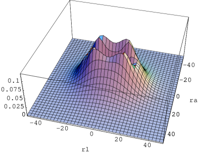
Figure 1: Conditional one-particle density function of the He₃ ground state, $r_{l}$, $r_{a}$ in Å

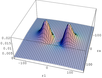
Figure 2: Conditional one-particle density function of the He₃ excited state, $r_{l}$, $r_{a}$ in Å

Omitting the integration over $z$ we define a conditional density function $\rho(r,z)$ that presents a spatial distribution for the particle 1 when the other two particles are located along the fixed axis. It is useful to plot this function in coordinates $(r_{l},r_{a})$ such that $r_{l}=rz$ is a projection of the particle 1 position to the axis connecting the other particles and $r_{a}=\frac{z}{|z|}r(1-z^{2})^{\frac{1}{2}}$ is a projection to the orthogonal axis. Three-dimensional plots of the function $\rho((r_{l}^{2}+r_{a}^{2})^{1/2},\cos\arctan\frac{r_{l}}{r_{a}})$ corresponding to the ground and excited states of the trimer calculated with LM2M2 potential are presented on the Fig. 1 and Fig. 2. The conditional density function of the ground state decreases democratically in all the directions. The density function of the excited state has two distinguishable maximums demonstrating the linear structure of the cluster. This structure has a simple physical explanation. The most probable positions of a particle in the excited state lie around two other particles. At the distances where two particles are well separated the third one forms a dimer-like bound state with each of them. This interpretation agrees with the clusterisation coefficients presented in the Tab. 4. These coefficients are calculated as a norm of the function $f_{c}$ defined as follows

$$f_{c}(y)=\int dx\,dz\,\Phi(x,y,z)\phi_{2}(x)\>,$$

where $\phi_{2}(x)$ is the dimer wave function. The values of $\|f_{c}(y)\|^{2}$ shown in the Tab. 5 demonstrate the dominating role of a two-body contribution to the trimer excited state whereas in the ground state this contribution is rather small. We could suppose that this dominating contribution of the cluster wave in the excited state has ensured fast convergence of the hyperspherical adiabatic expansion in the paper [11] to the correct value, but to get the same order of accuracy for the ground state possibly more basic functions should be taken into account.

Very demonstrative example of the advantage of Faddeev equations over the Schroedinger one in bound-state calculations is given in the Tabs. 8 and 9. Here we present the contribution of different angular states to the Faddeev component and to the wave function calculated as

$$\begin{array}[]{c}C_{n}=\|f_{n}(x,y)\|^{2}\\ \displaystyle f_{n}(x,y)=\int^{1}_{-1}dz\,F(x,y,z)P_{n}(z)\>,\end{array}$$

where $P_{n}(z)$ are the normalized Legendre polynomials, $F(x,y,z)$ is the Faddeev component or the wave function, $n=0,2,4$. The angular coefficients for the Faddeev component decrease much faster than the wave function coefficients. The Tab. 8 also demonstrates that more angular functions should be taken into account in the ground state calculations.

4 Conclusions

The high accuracy calculations of He₃ bound states were performed on the base of the most advanced few-body calculations techniques. Eight different potential models were used. For every potential model, either more (LM2M2, TTYPT) or less realistic one (LM2M2a, HFD-ID), two and only two bound states are found. The properties of these states are very different. The ground state is strongly bound, whereas the binding energy of the excited state is comparable with the binding energy of dimer. The sizes of these two states also differs much. The characteristic size of the ground state either estimated by $\langle r\rangle$ or $\langle r^{2}\rangle^{1/2}$ (Tabs. 5 and 6) is approximately 10 times less than the size of dimer molecule, but the size of the excited state has the same order of magnitude with the dimer’s one. This estimation shows the necessity to check for the absence of trimers in the experimental media during the measurement of dimer properties and vice versa.

List of tables

1. The energy of the He₂and He₃ bound states

2. Convergence of the He₃excited state energy with respect to the number of gridpoints

3. Convergence of the He₃ground state energy with respect to the number of gridpoints

4. Contribution of cluster wave to the Faddeev component

5. The mean square radius of Helium molecules

6. The mean radius of Helium molecules

7. Comparison with the results of other authors

8. Contribution of different two-body angular states to the Faddeev component

9. Contribution of different two-body angular states to the wave function

List of figures

1. Conditional one-particle density function of the He₃ ground state

2. Conditional one-particle density function of the He₃ excited state

3. He₃ ground state density function

4. He₃ excited state density function

5. He₂ density function

Table 1: The energy of the He₂ and He₃ bound states

Potential	$E_{2}$,mK	$\widetilde{E_{2}}$, mK	$E_{3}$, K	$E^{*}_{3}$, mK
HFD-A	-0.830124	-0.8305	0.11713	1.665
HFD-B	-1.685419	-1.68540	0.13298	2.734
HFD-ID	-0.40229	-0.4024	0.10612	1.06
LM2M1	-1.20909	-1.212	0.12465	2.155
LM2M2	-1.303482	-1.304	0.12641	2.271
LM2M1a	-1.52590	-1.527	0.13024	2.543
LM2M2a	-1.798436	-1.795	0.13471	2.868
TTY	-1.312262	-1.3121	0.12640	2.280

Table 2: Convergence of the He₃ excited state energy with respect to the number of gridpoints

Grid	$E^{*}_{3}$,Å${}^{-2}\times 10^{-5}$	$E_{2}$,Å${}^{-2}\times 10^{-5}$
45$\times$45$\times$9	-22.819	-14.123
60$\times$60$\times$9	-22.568	-13.913
60$\times$60$\times$15	-22.570	-13.913
75$\times$75$\times$9	-22.561	-13.907
75$\times$75$\times$15	-22.563	-13.907
90$\times$75$\times$9	-22.567	-13.912
105$\times$75$\times$9	22.555	-13.902

Table 3: Convergence of the He₃ ground state energy with respect to the number of gridpoints

Grid	$E_{3}$,Å${}^{-2}\times 10^{-5}$	$E_{2}$,Å${}^{-2}\times 10^{-5}$
45$\times$45$\times$15	-1096.35	-13.839
60$\times$60$\times$9	-1096.72	-13.894
60$\times$60$\times$15	-1097.11	-13.894
60$\times$60$\times$21	-1097.11	-13.894
105$\times$60$\times$18	-1097.19	-13.9062
105$\times$75$\times$15	-1097.25	-13.9062

Table 4: Contribution of cluster wave to the Faddeev component

Potential	$\|f_{c}\|^{2}$	$\|f_{c}^{*}\|^{2}$
HFD-A	0.2094	0.9077
HFD-B	0.2717	0.9432
HFD-ID	0.1555	0.8537
LM2M1	0.2412	0.9283
LM2M2	0.2479	0.9319
LM2M1a	0.2624	0.9390
LM2M2a	0.2780	0.9458
TTY	0.2487	0.9323

Table 5: The mean square radius of Helium molecules, Å

Potential	Ground state of He3	Excited state of He3	He2
HFD-A	6.46	66.25	88.18
HFD-B	6.23	57.89	62.71
HFD-ID	6.64	75.38	126.73
LM2M1	6.35	61.74	73.54
LM2M2	6.32	60.85	70.93
LM2M1a	6.27	59.03	65.76
LM2M2a	6.21	57.17	60.79
TTYPT	6.33	60.81	70.70

Table 6: The mean radius of Helium molecules, Å

Potential	Ground state of He3	Excited state of He3	He2
HFD-A	5.65	55.26	64.21
HFD-B	5.48	48.33	46.18
HFD-ID	5.80	62.75	91.50
LM2M1	5.57	51.53	53.85
LM2M2	5.55	50.79	52.00
LM2M1a	5.51	49.28	48.34
LM2M2a	5.46	47.72	44.82
TTYPT	5.55	50.76	51.84

Table 7: Comparison with the results of other authors

Observable	This work	[8]	[9]	[7]	[10]
HFD-A(He)
$E_{3}$, K	-0.1171	-0.117	-0.114	-0.11	-0.107
$E^{*}_{3}$, mK	-1.665		-1.74	-1.6
HFD-B(He)
$E_{3}$, K	-0.1330		-0.132		-0.130
$E_{3}^{*}$, mK	-2.734		-2.83

LM2M2
Observable	This work	[11]	[12]
$E_{3}$, K	-0.1264	-0.1252	-0.219
$E^{*}_{3}$, mK	-2.271	-2.269	-1.73
$<r^{2}>^{1/2}$, Å	6.32	6.24	7.4
$<r^{2}_{*}>^{1/2}$, Å	60.85	60.86	50.3

Table 8: Contribution of different two-body angular states to the Faddeev component

	Ground state			Excited state
Potential	S	D	G	S	D	G
HFD-A	0.9991043	0.0008859	0.0000095	0.9999964	0.0000035	0.0000000
HFD-B	0.9990000	0.0009890	0.0000107	0.9999952	0.0000048	0.0000001
HFD-ID	0.9991709	0.0008200	0.0000088	0.9999972	0.0000028	0.0000000
LM2M1	0.9990505	0.0009390	0.0000101	0.9999958	0.0000042	0.0000000
LM2M2	0.9990393	0.0009500	0.0000103	0.9999957	0.0000043	0.0000000
LM2M1a	0.9990129	0.0009762	0.0000105	0.9999954	0.0000046	0.0000001
LM2M2a	0.9989834	0.0010053	0.0000109	0.9999950	0.0000049	0.0000001
TTY	0.9990332	0.0009561	0.0000104	0.9999956	0.0000043	0.0000000

Table 9: Contribution of different two-body angular states to the wave function

	Ground state			Excited state
Potential	S	D	G	S	D	G
HFD-A	0.95416	0.03198	0.00877	0.90957	0.07543	0.01331
HFD-B	0.95193	0.03365	0.00947	0.89710	0.08546	0.01546
HFD-ID	0.95493	0.03116	0.00905	0.91919	0.06763	0.01170
LM2M1	0.95323	0.03277	0.00891	0.90337	0.08043	0.01437
LM2M2	0.95303	0.03294	0.00893	0.90201	0.08152	0.01460
LM2M1a	0.95259	0.03332	0.00899	0.89904	0.08391	0.01512
LM2M2a	0.95210	0.03374	0.00906	0.89574	0.08654	0.01569
TTY	0.95245	0.03318	0.00941	0.90186	0.08164	0.01463

Figure 3: He₃ ground state density function, $r$ in Å

Figure 4: He₃ excited state density function, $r$ in Å

Figure 5: He₂ dimer density function, $r$ in Å

References

- [1] W.Schöllkopf and J.P.Toennies J. Chem. Phys. 104(3), 1155, (1996)
- [2] F. Luo, C. F. Giese and W. R. Gentry J. Chem. Phys. 104(3), 1151, (1996)
- [3] J. C. Mester, E. S.Meyer, M. W. Reynolds, T.E. Huber, Z. Zhao, B. Freedman, J. Kim and I.F.Silvera Phys. Rev.Lett. 71(9), 1343, (1993)
- [4] V. Efimov, Phys.Lett. B 33, 563 (1970)
- [5] T. K. Lim and M.A.Zuniga J. Chem. Phys. 63(5), 2245, (1974)
- [6] T. K. Lim, S.K. Duffy and W.C.Damert Phys. Rev.Lett. 38(7), 341, (1977)
- [7] Th. Cornelius, W. Glöckle, J. Chem. Phys., 85, 3906 (1986)
- [8] V. R. Pandharipande, J. G. Zabolitzky, S. C. Pieper, R. B. Wiringa, and U. Helmbrecht, Phys. Rev. Lett., 50, 1676 (1983).
- [9] E. A. Kolganova, A. K. Motovilov, S.A. Sofianos LANL E-print chem-ph/9612012
- [10] J. Carbonell, C. Gignoux, S. P. Merkuriev, Few–Body Systems 15, 15 (1993).
- [11] E. Nielsen, D. V. Fedorov and A. S. Jensen, LANL e-print physics/9806020
- [12] T. Gonzalez-Lezana, J.Rubayo-Soneira, S.Miret-artes, F.A. Gianturco, G. Delgado-Barrio and P.Villarreal, Phys.Rev.Lett, 82(8), 1648, (1999)
- [13] V. Roudnev and S. Yakovlev, Proceedings of the first international conference Modern Trends in Computetional Physics, (1998), to be published in Comp. Phys. Comm.
- [14] L. D. Faddeev, S. P. Merkuriev, Quantum scattering theory for several particle systems (Doderecht: Kluwer Academic Publishers, (1993)).
- [15] V. V. Kostrykin, A. A. Kvitsinsky,S. P. Merkuriev Few-Body Systems, 6, 97, (1989)
- [16] N. W. Schellingerhout, L. P. Kok, G. D. Bosveld Phys. Rev. A 40, 5568-5576, (1989)
- [17] B. Liu and A. D. McLean, J. Chem. Phys. 91(4), 2348 (1989)
- [18] R. A. Aziz, V. P. S. Nain, J. S. Carley, W. L. Taylor, and G. T. McConville, J. Chem. Phys. 70, 4330 (1979).
- [19] R. A. Aziz, F. R. W. McCourt, and C. C. K. Wong, Mol. Phys. 61, 1487 (1987).
- [20] R. A. Aziz and M. J. Slaman, J. Chem. Phys. 94, 8047 (1991).
- [21] T. van Mourik and J. H. van Lenthe, J. Chem. Phys. 102(19), 7479 (1995)
- [22] K.T.Tang, J. P. Toennis and C. L. Yiu Phys. Rev.Lett. 74(9), 1546, (1995)
- [23] J. B. Anderson, C.A. Traynor and B. M. Boghosian, J. Chem. Phys. 99(1),345 (1993)