Quasi-Chemical Theory
and
Implicit Solvent Models for Simulations

Abstract

A statistical thermodynamic development is given of a new implicit solvent model that avoids the traditional system size limitations of computer simulation of macromolecular solutions with periodic boundary conditions. This implicit solvent model is based upon the quasi-chemical approach, distinct from the common integral equation trunk of the theory of liquid solutions. The idea is geometrically to define molecular-scale regions attached to the solute macromolecule of interest. It is then shown that the quasi-chemical approach corresponds to calculation of a partition function for an ensemble analogous to, but not the same as, the grand canonical ensemble for the solvent in that proximal volume. The distinctions include: (a) the defined proximal volume — the volume of the system that is treated explicitly — resides on the solute; (b) the solute conformational fluctuations are prescribed by statistical thermodynamics and the proximal volume can fluctuate if the solute conformation fluctuates; and (c) the interactions of the system with more distant, extra-system solution species are treated by approximate physical theories such as dielectric continuum theories. The theory makes a definite connection to statistical thermodynamic properties of the solution and fully dictates volume fluctuations, which can be awkward in more ambitious approaches. It is argued that with the close solvent neighbors treated explicitly the thermodynamic results become less sensitive to the inevitable approximations in the implicit solvent theories of the more distant interactions. The physical content of this theory is the hypothesis that a small set of solvent molecules are decisive for these solvation problems. A detailed derivation of the quasi-chemical theory escorts the development of this proposal. The numerical application of the quasi-chemical treatment to Li⁺ ion hydration in liquid water is used to motivate and exemplify the quasi-chemical theory. Those results underscore the fact that the quasi-chemical approach refines the path for utilization of ion-water cluster results for the statistical thermodynamics of solutions.

Introduction

Direct simulation of macromolecules in aqueous solutions typically requires consideration of a mass of solution large compared to the mass of the macromolecular solute. Frequently, the bulk of the solution is of secondary interest. The extravagant allocation of computational resources for direct treatment of macromolecular solutions limits the scientific problems that may be tackled. Thus, implicit solvent models that eliminate the direct presence of the solvent in favor of an approximate description of the solvation effects have received universal and extended interest Berkowitz:82 ; Brooks:83 ; Brunger:84 ; Belch:85 ; Brooks:85 ; Brooks:86 ; Pratt:86 ; Brunger:87 ; Brooks:89 ; Brooks:88 ; Deloof:91 ; Levchuk:91 ; Shiratori:91 ; Straub:91 ; Braatz:92 ; Tapia:92 ; Widmalm:92 ; Heller:93 ; Fritsch:93 ; Juffer:93 ; Nakagawa:93 ; Rashin:93 ; Beglov:94 ; Arnold:94 ; Axelsen:94 ; Davis:94 ; Lazaridis:94 ; Pastor:94 ; Straub:94 ; Sharp:94 ; Beglov:95 ; Eriksson:95 ; Essex:95 ; Norberg:95 ; Alaman:96 ; Bencsura:96 ; David:96 ; Larwood:96 ; Luty:96 ; Wang:96 ; Albaret:97 ; Haggett:97 ; Han:97 ; Meirovitch:97 ; Parrill:97 ; Merz:98 ; Zeng:98 ; Lounnas:99 ; Prabhu:99 ; Roux:99a ; Roux:99b ; Roux:99c ; Levy:99 .

These issues are specifically relevant to this workshop on electrostatic interactions in solution for two reasons. First, electrostatic interactions exacerbate the difficulties of solute size mentioned above. If all interactions were short-ranged, most practitioners would be satisfied with the traditional approach, adopting periodic boundary conditions and empirically examining the system size dependence of their results by performing calculations on successively larger systems. Second, the additional computational requirements to treat genuinely chemical phenomena in solution by in situ electronic structure calculations again limits the problems that can be addressed. In fact, the principal physical concepts involved in electronic structure calculations for chemical problems in liquid water universally involve electrostatic interactions of long range. The important example of metal ion chemistry in proteins combines these points.

Although a variety of implicit solvent models have been tried by now in numerous selected applications, they are still limited in fundamental aspects. A helpful recent discussion of important limitations was given by Juffer and BerendsenJuffer:93 . They emphasize that implicit solvent models should be significantly simpler than explicit models in view of the approximations and ad hoc features that are accepted. Solution chemistry problems that require direct treatment of electronic degrees of freedom are one kind of problem that must be made significantly simpler to permit a broader computational attack. A striking example is the current ‘ab initio’ molecular dynamics calculations of aqueous solutions of simple ions. They do treat electronic structure issues within simulations but have been typically limited to total system sizes of 16 – 32 water molecules in periodic boundary conditionsmarx:99 , small systems by current standards with classical simulation models. These small sizes do limit the conclusions that might be drawn; the structure and dynamics of the second hydration shell of a Li⁺ ion in liquid water, the example discussed below, undoubtedly requires calculation on systems larger than 32 water molecules. Nevertheless, much can be learned from the study of such small systems, particularly when chemical effects of the interactions of a solute with proximal solvent molecules are the issues of greatest importancelubin:99 .

The idea for the developments presented here is aggressively to adopt the Juffer-Berendsen suggestion that implicit solvent models must be significantly simpler than explicit models and apply that philosophy to the statistical thermodynamic treatment of aqueous solutions. To that end, we acknowledge that some water molecules play a specific, almost chemical, role in these hydration phenomena. We then work out the theory that permits inclusion of a small number of such molecules explicitly. The required theory is a descendent of the quasi-chemical approximations of GuggenheimGuggenheim:35 , BetheBethe:35 , and Kikuchibrush . It is a significant simplification of direct simulation calculations. Roughly described, that theory organizes and justifies treatment of a handful of water molecules essentially as ligands of the macromolecule of interest, letting the more distant solution environment be treated by simple physical approximations such as the popular dielectric continuum models.

The plan of this presentation is first to introduce an example, the hydration of the Li⁺ ion, that permits a convenient discussion of the quasi-chemical theory. That example illustrates the quasi-chemical pattern for the theory, exemplifies the basic molecular information required to construct quasi-chemical predictions, and offers a simplified derivation based upon a thermodynamic model. Following that we give an extended theoretical development of the quasi-chemical organization of calculations of solvation free energies and then use those theoretical results to suggest an explicit-implicit solvent model for statistical thermodynamic calculations of solutions.

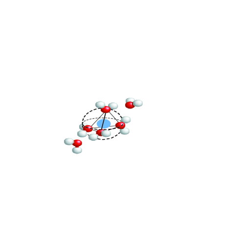
Figure 1: The minimum energy structure of a Li⁺ ion with six water molecules. The inscribed ball identifies the inner shell occupied by the four nearest water molecules. The two further water molecules are in an outer shell. This illustrates the definition of the bonding or inner shell region.

Example: the Li⁺ Ion in Water

The hydration of atomic ions provides a conceptually simple context in which to consider the quasi-chemical approaches developed below. The previous study of the hydration of ferric ion, Fe³⁺(aq), provides one such exampleMartin:98 . Here we motivate the formal developments of the theory by considering the hydration of the Li⁺ ion in dilute aqueous solution and we will discuss the principal theoretical structures in this context first. We anticipate some of the discussion below by noting that Li⁺(aq) proves to be a difficult case in some important respects. Thus, we expect to return to this example in later work. Indeed, the goal of the theoretical developments initiated here is of a sufficiently constructive nature that all pieces of the puzzle needn’t become available at the same time!

Quasi-chemical Structure for the Hydration Free Energy

The quasi-chemical theory suggests expressing the chemical potential of the lithium ion species, $\mu_{Li^{+}}$, in terms of ideal and non-ideal, or interaction, contributions:

$$\beta \mu_{Li^{+}}=\ln\left[{{{\rho_{Li^{+}}}\over{q_{Li^{+}}/V}}}\right]-\ln p_{0}-\ln\left[\sum\limits_{n\geq 0}{\tilde{K}_{n}}\,\rho_{H_{2}O}{}^{n}\right],$$ (1)

with $\beta^{-1}=RT$. In the last contribution, only a limited number of terms are included in the sum. That limited number is the maximum number of water molecules that may occur as inner hydration shell ligands. For the Li⁺ ion example, that limited number need not be greater than six (6). Fig. 1 shows the minimum energy structure of the Li⁺ ion with six water moleculesrempe:99 .

The coefficients ${\tilde{K}_{n}}$ of Eq. (1) will be defined more fully later. A virtue of this approach is that the natural initial approximation is ${\tilde{K}_{n}}\approx K_{n}^{(0)}$, the equilibrium ratio for the reactions that form various inner shell clusters

$$Li^{+}\ +\ nH_{2}O\rightleftharpoons Li^{+}(H_{2}O)_{n}$$ (2)

without consideration of medium effects, as for an ideal gas. Those coefficients can be assembled within the harmonic approximation for the cluster vibrations utilizing standard electronic structure computational packagesgbook . That idea is reinforced by the results in Tables 1, 2, and 3, which we use to develop this examplerempe:99 .

Table 1: Electronic energy (E), zero-point energy (ZPE), the interaction part of the chemical potential ($\mu^{*}$) for Li(H₂O)${}_{n}{}^{+}$ complexes, and the Mulliken charge for the Li⁺ ion in each complex utilizing the B3LYP and dielectric continuum solvation approximations. Geometries and ChelpG partial charges were obtained with basis 6-31++G** for O, H, and 6-31G* for Li⁺. The Mulliken partial charges were obtained with the smaller basis 6-31G on all atoms in order to simplify their consideration. Dielectric radii for all atoms were taken from Ref. Stefanovich except R${}_{Li^{+}}$=2.0 Å.

	$E(au)$	$ZPE(kcal/mol)$	$\mu^{*}(kcal/mol)$	$\delta(e)$
H2O	$-76.4332$	$13.4$	$-8.3$	$-$
Li+	$-7.2845$	$-$	$-82.$	$1.0$
Li(H2O)+	$-83.7750$	$15.5$	$-73.$	$0.9$
Li(H2O)${}_{2}^{+}$	$-160.2596$	$31.0$	$-68.$	$0.7$
Li(H2O)${}_{3}^{+}$	$-236.7308$	$46.5$	$-65.$	$0.6$
Li(H2O)${}_{4}^{+}$	$-313.1912$	$61.4$	$-65.$	$0.5$
Li(H2O)${}_{5}^{+}$	$-389.6390$	$76.7$	$-63.$	$0.4$
Li(H2O)${}_{6}^{+}$	$-466.0878$	$93.0$	$-61.$	$0.3$

Within the quasi-chemical approximation of collective phenomenabrush , the factors of solvent density that appear explicitly in Eq. (1) can be recognized as mean-field estimates of the influence of the solvent on the chemical potential of the Li⁺(aq) ion. That form of the solvent mean field, however, derives from specific compositional effects. For the realistic circumstances that long-ranged interactions of the classic electrostatic type are important, the approximation ${\tilde{K}_{n}}\approx K_{n}^{(0)}$ should be revised with implicit solvent theories intended to describe the influence of the more distant solution environment on the chemical potential of the Li⁺(aq) ion. This hints at the strategy for the quasi-chemical approaches. Neighbors occupying a carefully defined proximal volume are treated explicitly. But more distant neighbors are treated implicitly with the view that they can be satisfactorily treated with simple theories and, in any case, those more distant effects are a smaller part of the whole.

Table 2: Ideal gas thermochemistries (kcal/mole) at T=298.15 K and p=1 atm, using the B3LYP functionalG98 . The first column gives the electronic energy contribution, the second the zero-point energy, the third the energy, the fourth the enthalpy, and the fifth column is the Gibbs free energy, all at 298.15 K.

	${\Delta}E_{e}$	${\Delta}E{{}_{0}}$	${\Delta}E_{298}^{(0)}$	${\Delta}H_{298}^{(0)}$	${\Delta}G_{298}^{(0)}$
Li++H2O $\rightarrow$ Li(H2O)+	$-35.9$	$-33.8$	$-33.4$	$-33.4$	$-36.0$
Li(H2O)++H2O $\rightarrow$ Li(H2O)2+	$-32.2$	$-30.1$	$-29.9$	$-30.4$	$-22.5$
Li(H2O)${}_{2}^{+}$+H2O $\rightarrow$ Li(H2O)3+	$-23.8$	$-21.7$	$-21.5$	$-22.1$	$-13.5$
Li(H2O)${}_{3}^{+}$+H2O $\rightarrow$ Li(H2O)4+	$-17.1$	$-15.5$	$-15.0$	$-15.5$	$-7.5$
Li(H2O)${}_{4}^{+}$+H2O $\rightarrow$ Li(H2O)5+	$-9.2$	$-7.3$	$-7.1$	$-7.7$	$2.1$
Li(H2O)${}_{5}^{+}$+H2O $\rightarrow$ Li(H2O)6+	$-9.8$	$-6.9$	$-7.3$	$-7.9$	$4.0$

The quantity -$\ln p_{0}$ of Eq. (1) gives the free energy in units $\beta^{-1}$ required to open this defined proximal volume in the solvent in order that the construction of the complexes of Eq. (2) can be pursued. This quantity is an object of research in the theory of liquids pratt:99 in its own right. For specific applications an approximate form must be used. In the present example of the hydration of the Li⁺ ion, this packing contribution is expected to be of a secondary size, provided the thermodynamic state is not varied too broadly.

Finally, the quantity $q_{Li^{+}}$ of Eq. (1) is the canonical partition function for a single Li⁺ in a volume V at temperature Tmcq . The initial term of Eq. (1) is recognized as the ideal (no interactions) contribution to $\mu_{Li^{+}}$. Thus, the second and third terms there express the interactions of the Li⁺ ion with the solvent and we will refer to these contributions as $\beta\Delta\mu_{Li^{+}}$.

As a point of reference, for the present example of the Li⁺ at infinite dilution in water under the normal conditions of T=298.15 K and $\rho_{W}$=1 g/cm³, we calculate the quasi-chemical contributions (the last term) to Eq. (1) to be -128 kcal/mole using R${}_{Li^{+}}$=2.0Å. The experimental values for the total $\Delta\mu_{Li^{+}}$ are -114 kcal/molmarcus and -125 kcal/molFriedman:73 . The contributions of repulsive interactions will raise that calculated value toward the experimental whole, but it is unlikely to raise it enough to exceed the highest of these values. Though the agreement is satisfactory, it seems likely that the calculated result is too low, meaning that the Li⁺ ion is less well bound to liquid water than the current calculation predicts. Additionally, the clusters have been treated in the harmonic approximation in obtaining this theoretical valuerempe:99 .

Table 3: Construction of aqueous solution thermochemical results (kcal/mole) at T=298.15 K. The first column gives the gas-phase free energy from Table 2 for the sequential hydration reactions, the second reports the reaction net free energy after adjustment for the actual concentration of liquid water, and the third column gives the interaction part of the chemical potential change, $\Delta\mu^{*}=\mu^{*}_{Li(H_{2}O)_{n}{}^{+}}-\mu^{*}_{H_{2}O}-\mu^{*}_{Li(H_{2}O)_{n-1}{}^{+}}$, for n=$1,2,\ldots 6$, approximated with the dielectric model. The fourth column is the total free energy change for the indicated reaction in aqueous solution, the sum of the second and third columns. To construct the results of Fig. 2, use $\mu^{*}_{Li^{+}}\approx$ -82.0 kcal/mol, the Born model result for R${}_{Li^{+}}$=2.0 Å.

	${\Delta}G_{298}^{(0)}$	${\Delta}G_{298}$	${\Delta}\mu^{*}$	${\Delta}G_{298}(aq)$
Li++H2O $\rightarrow$ Li(H2O)+	$-36.0$	$-40.3$	$17.3$	$-23.0$
Li(H2O)++H2O $\rightarrow$ Li(H2O)2+	$-22.5$	$-26.8$	$13.3$	$-13.5$
Li(H2O)${}_{2}^{+}$+H2O $\rightarrow$ Li(H2O)3+	$-13.5$	$-17.8$	$11.3$	$-6.5$
Li(H2O)${}_{3}^{+}$+H2O $\rightarrow$ Li(H2O)4+	$-7.5$	$-11.7$	$8.3$	$-3.4$
Li(H2O)${}_{4}^{+}$+H2O $\rightarrow$ Li(H2O)5+	$2.1$	$-2.2$	$10.3$	$8.1$
Li(H2O)${}_{5}^{+}$+H2O $\rightarrow$ Li(H2O)6+	$4.0$	$-0.3$	$10.3$	$10.0$

A Thermodynamic Model

One physical view of the quasi-chemical approach is the following: Li⁺ ions in aqueous solution can, in principal, be polled for the number $n$ of water molecule ligands each possesses. We could determine the concentrations of Li⁺ ions having precisely $n$ water molecule ligands. In fact, the $n^{th}$ term in the sum of Eq. (1) is proportional to those concentrations. Denoting the mole fraction of Li⁺ ions with $n$ water molecule ligands by $x_{n}$, successive terms there can be expressed as $x_{n}\exp(-\beta\Delta\mu_{Li^{+}})$Pratt:98 . Those mole fractions, however, are not independent thermodynamic variables but are governed by the principles of chemical equilibrium. In our example of Li⁺(aq), the quasi-chemical theory predicts the mole fractions of Li⁺ ions with $n$ water molecule ligands, as is shown in Fig. 2.

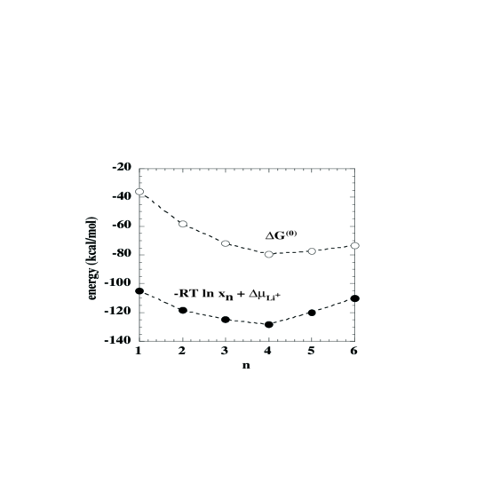
Figure 2: Free energies for Li⁺(aq) ion hydration in liquid water plotted as a function of the number, $n$, of inner shell water neighbors, T=298.15 K; see Table 3. The results marked $\Delta$G⁽⁰⁾ are the free energies predicted by the electronic structure calculations for the reaction Li⁺ + $n$H₂O = Li(H₂O)${}_{n}{}^{+}$ under standard ideal conditions, including p = 1 atm. The minimum value is at $n$=4. The solid circles labeled -RT$\,\ln\,x_{n}\,+\Delta\mu_{Li^{+}}$ are the final, net values that include the $\rho_{H_{2}O}{}^{n}$ factors of Eq. (1) adjusting the water molecule concentration from the ideal case to the actual concentration of liquid water, and the extra-cluster interaction contributions of Eq. (36). The final results predict that the $n$=4 inner sphere structure is most probable in liquid water under normal conditions.

These ideas can be the basis of an unrefined but almost thermodynamical derivation of the pattern in Eq. (1). To develop this ‘derivation’, we first make explicit that we consider the concentrations of the Li(H₂O)${}_{n}^{+}$ complexes of different size $n$ despite the fact that it is the concentration of Li⁺ ions that can be experimentally manipulated. Thus, we introduce a new set of composition variables that refer to the ion complexes,

$$N_{Li^{+}} = \sum\limits_{n\geq 0}{{\tilde{N}}_{Li\left({H_{2}O}\right)_{n}^{+}}},$$

$$N_{H_{2}O} = \tilde{N}_{H_{2}O}+\sum\limits_{n\geq 0}{n\tilde{N}_{Li\left({H_{2}O}\right)_{n}^{+}}}.$$ (3)

Here the total number of each species in solution, $N_{Li^{+}}$ and $N_{H_{2}O}$, is expressed in terms of ${\tilde{N}}_{Li\left({H_{2}O}\right)_{n}^{+}}$, the numbers of complexes of different sizes $n$, and ${\tilde{N}}_{H_{2}O}$, the number of water molecules not complexed to an ion.

For the problem initially addressed in terms of variables $N_{H_{2}O}$ and $N_{Li^{+}}$, these relations provide a translation to express the problem in terms of an alternative set of variables such as $\tilde{N}_{H_{2}O}$ and $\tilde{N}_{Li\left({H_{2}O}\right)_{n}^{+}}$. In the formal definition of the Gibbs free energy $G$, for example, with these changes of variables the multiplier of $\tilde{N}_{Li\left({H_{2}O}\right)_{n}^{+}}$ becomes $\left(\mu_{Li^{+}}+n\mu_{H_{2}O}\right)$. If the molecule number $\tilde{N}_{Li\left({H_{2}O}\right)_{n}^{+}}$ could be varied independently of other such composition variables, we would identify this multiplier as the chemical potential conjugate to $\tilde{N}_{Li\left({H_{2}O}\right)_{n}^{+}}$. In contrast, for the problem initially formally addressed in terms of variables like $\tilde{N}_{H_{2}O}$ and $\tilde{N}_{Li\left({H_{2}O}\right)_{n}^{+}}$, as we do here, then the relative concentrations, $x_{n}={{\tilde{N}}_{Li\left({H_{2}O}\right)_{n}^{+}}}/N_{Li^{+}}$, provide a translation to the problem expressed in terms of the standard variables such as $N_{H_{2}O}$ and $N_{Li^{+}}$. The coefficient of $N_{Li^{+}}$ in the Gibbs free energy expression is

$$\sum\limits_{n\geq 0}{x_{n}\left({\tilde{\mu}_{Li\left({H_{2}O}\right)_{n}^{+}}-n{\tilde{\mu}}_{H_{2}O}}\right)}\equiv\mu_{Li^{+}},$$ (4)

the thermodynamic chemical potential conjugate to $N_{Li^{+}}$. The differences within the parenthesis depend on relative concentrations of complexes of different sizes. These relative concentrations are established by nontrivial conditions of equilibrium.

To show the consequences of those conditions of equilibrium, we adopt the standard form of the chemical potential, 

$$\beta\mu_{\sigma}=\ln\left[\rho_{\sigma}V/q_{\sigma}\right],$$ (5)

so that

$$\beta\mu_{Li^{+}}=\sum\limits_{n\geq 0}{x_{n}\ln\left[{\rho_{Li^{+}}x_{n}(q_{H_{2}O}/V){}^{n}\over\rho_{H_{2}O}{}^{n}(q_{Li\left({H_{2}O}\right)_{n}^{+}}/V)}\right]}.$$ (6)

The final essential step in this thermodynamic model is the quasi-chemical step according to which the relative concentrations of the ion complexes of different sizes are expressed as a function of the chemical equilibrium constants,

$$x_{n}={{K_{n}^{(0)}\rho_{H_{2}O}{}^{n}}\over{\sum\limits_{m\geq 0}{K_{m}^{(0)}\rho_{H_{2}O}{}^{m}}}}.$$ (7)

Consistent with the notation above, chemical equilibrium requires that

$$K_{n}^{(0)}={{\left({q_{Li(H_{2}O)_{n}^{+}}/V}\right)}\over{\left({q_{Li(H_{2}O)_{n=0}^{+}}/V}\right)\left({q_{H_{2}O}/V}\right)^{n}}}.$$ (8)

The K${}_{n}^{(0)}$ are a function of the temperature T as the only thermodynamic variable. When the results above are collected, we remember that the x_n are non-negative weights that sum to one and we notice that $q_{Li^{+}}=q_{Li(H_{2}O)_{n=0}^{+}}$ so that we can separate the correct ideal contribution to $\mu_{Li^{+}}$. Thus the chemical potential of the lithium ion separates into ideal and non-ideal contributions, with the latter contribution written in terms of the equilibrium ratios K${}_{n}^{(0)}$ that appeared in Eq. (1),

$$\beta\mu_{Li^{+}}=\ln\left[{\rho_{Li^{+}}\over(q_{Li^{+}}/V)}\right]-\ln\left[\sum\limits_{n\geq 0}{K_{n}^{(0)}\rho_{H_{2}O}{}^{n}}\right].$$ (9)

Within the simplified context of this derivation, this is the result that was sought.

The previous equation should be compared with Eq. (1). Note that it doesn’t address the initial packing contribution -$\ln p_{0}$, or the other extra-cluster interaction contributions incorporated into ${\tilde{K}}_{n}$ of Eq. (1). Furthermore, it finesses the recognition issue of defining cluster structures for counting. Nevertheless, we can note that the quasi-chemical step, Eq. (7), would arise in a pedagogical context by making the free energy stationary with respect to variations in the progress of chemical reactions. Because of this variational aspect these approaches are sometimes referred to as cluster-variation theoriesbrush .

Variations of Hydration Free Energies

Predictions of variations of hydration free energy changes with temperature, pressure, composition, and solute geometry are the foremost practical weaknesses of dielectric continuum models for hydration free energies. An important facet of this issue is that the radii parameters in the dielectric models, which are initially established fully empirically, depend on solution thermodynamic conditions such as temperature, pressure, and composition, and on solute conformationPratt:94a ; Tawa:94 ; Tawa:95 ; Pratt:97 ; Hummer:98 . The Li⁺(aq) case gives direct example of this difficulty: the partial molar volume of the Li⁺(aq) is negative, -6.4 cm³/molmarcus . The magnitude of this important thermodynamic quantity is not explicable simply on the basis of the Born modelmarcus and the sign cannot be rationalized either if any reasonable description of excluded volume effects is included. At this point, considerable further evolution of dielectric models typically occurs with additional empirical parametersmarcus ; Floriano:98 . In contrast, an important feature of the present approach is that explicit contributions to the temperature and density dependences of the chemical potential are readily available. This facilitates investigation of thermodynamic derivatives.

Pressure Variation of Hydration Free Energies

The variation of the hydration free energies with pressure is the partial molar volume and gives direct information on hydration structure. Thus, it is particularly valuable in learning about the hydration process. Recalling that the chemical potential expression used in the current approach is written explicitly in Eq. (1), the partial molar volume $\left.{\left(\partial V/\partial N_{Li^{+}}\right)}\right|_{\beta,p,N_{H_{2}O}}$ is

$$v_{Li^{+}} \equiv \left.{\left({{{\partial\mu_{Li^{+}}}\over{\partial p}}}\right)}\right|_{\beta,N_{H_{2}O,}N_{Li^{+}}}$$ (10)

$$= {1\over\rho_{Li^{+}}}\left.\left({\partial\rho_{Li^{+}}\over\partial\beta p}\right)\right|_{\beta,N_{H_{2}O},N_{Li^{+}}}+\left({\partial\beta\Delta\mu_{Li^{+}}\over\partial\rho_{H_{2}O}}\right)_{\beta,\rho_{Li^{+}}}\left.\left({\partial\rho_{H_{2}O}\over\partial\beta p}\right)\right|_{\beta,N_{H_{2}O},N_{Li^{+}}}.$$

Here we are interested exclusively in the conditions of infinite dilution of the aqueous solution so that

$$\lim_{\rho_{Li^{+}}\rightarrow 0}v_{Li^{+}}=(\kappa_{T}/\beta)\left[{1+\rho_{H_{2}O}\left({{{\partial\beta\Delta\mu_{Li^{+}}}\over{\partial\rho_{H_{2}O}}}}\right)_{\beta}}\right],$$ (11)

where $\kappa_{T}$ = $(-1/V)\left(\partial V/\partial p\right)_{T}$ is the isothermal coefficient of bulk compressibility of the pure solvent. Upon differentiation, the first two terms of Eq. (1) produce the partial molar volume of a hard inert sphere of the right size at infinite dilution; call it $v_{0}$. As indicated above this is a topic of separate studypalma:93 . Thus,

$$\lim_{\rho_{Li^{+}}\rightarrow 0}\,v_{Li^{+}} = v_{0}-(\rho_{H_{2}O}RT\kappa_{T})\left({\partial\over\partial\rho_{H_{2}O}}\right)_{\beta}\ln\left[\sum\limits_{n\geq 0}{\tilde{K}_{n}}\,\rho_{H_{2}O}{}^{n}\right].$$ (12)

If the initial approximation ${\tilde{K}_{n}}\approx K_{n}^{(0)}$ is retained, or more generally if the extra-complex, or implicit solvent parts are only weakly density dependent, then the derivative indicated in Eq. (12) can be evaluated explicitly. Within this approximate view, the formula in Eq. (12) can be given a direct interpretation. We can parse the final term in Eq. (12) as

$$\Delta v=(\kappa_{T}\rho_{H_{2}O}RT)\;v_{H_{2}O}\;{\overline{n}}$$ (13)

where $v_{H_{2}O}=1/\rho_{H_{2}O}$ is the partial molar volume of the pure solvent (water) and

$${\overline{n}}=\left({\partial\over\partial\ln\rho_{H_{2}O}}\right)_{\beta}\ln\left[\sum\limits_{n\geq 0}{\tilde{K}_{n}}\,\rho_{H_{2}O}{}^{n}\right]=\sum\limits_{n\geq 0}nx_{n}.$$ (14)

The leading factor $\rho_{H_{2}O}RT\kappa_{T}$ appropriately converts a density change to a pressure change. The following factors assess the volume change per ligand and the number of ligands. This interpretation doesn’t work in this specific sense if the density dependence of the coefficients in Eq. (14) is significant. (It is interesting to note, however, the more general interpretation given by References Matubayasi:94 ; Matubayasi:96 to the partial molar quantities.)

We find ${\overline{n}}$ = 4.0, as demonstrated in Fig. 2 in the present example of the Li⁺ at infinite dilution in water under the normal conditions of T=298.15 K and $\rho_{W}$=1 g/cm³. As depicted in Fig. 3, the value ${\overline{n}}$ = 4.0 has been corroborated by ‘ab initio’ molecular dynamics calculationsrempe:99 . Combined with the other factors, ${\overline{n}}$ = 4.0 produces a contribution of -4.9 cm³/mole to the partial molar volume of Eq. (13). The simplest idea for estimation of the non-electrostatic contributions is to use the experimental value for the partial molar volume of He as a solute in water, 14.8 cm³/moleclever , making the total predicted partial molar volume of Li⁺ $v_{Li^{+}}$=9.9 cm³/mole. Therefore, this pain-staking accounting of the effects through the first hydration shell, detailed though it is, does not satisfactorily explain the partial molar volume of Li⁺ in liquid water. Since Li⁺(aq) is known to have a strongly structured second hydration shellHeinzinger:79 ; Mezei:81 ; Impey:83 ; Chandrasekhar:84 ; bounds:85 ; Zhu:91 ; Romero:91 ; lee:94 ; toth:96 ; Koneshan:98b , use of the dielectric model for the interactions of the Li⁺ with the outer hydration shells is a concern and may account for the difference between the calculated and experimental partial molar volumes.

We note that Eq. (13) assumes that the implicit contributions to the pressure variation are negligible. Use of the Born model directly without an empirical attribution of pressure dependence to the Born radii but with the measured pressure dependence of the solvent dielectric constantnbs contributes -0.3 cm³/mol, a negligible magnitude here. The density dependences of hydration free energies for the auto-dissociation reaction $2H_{2}O\rightleftharpoons H_{3}O^{+}+OH^{-}$ in water were studied some time agoTawa:95 from the point of view of a dielectric continuum model with the conclusion that a non-trivial density dependence was required of the dielectric model by the experimental data. In contrast, the formula Eq. (13) is properly insensitive to radii parameters assigned to the solute.

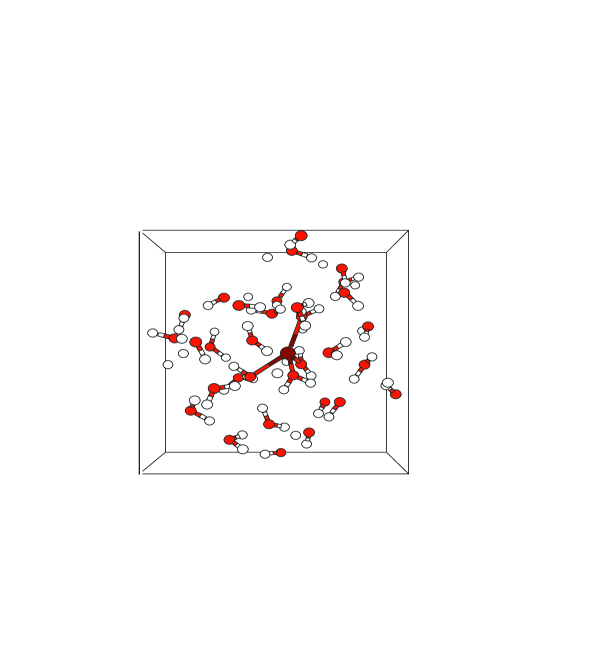
Figure 3: A structure from ‘ab initio’ molecular dynamics calculations based upon a gradient-corrected electron density functional description of the interatomic forces, after Ref. rempe:99 . Initially a hexa-coordinate inner sphere structure, rigidly constrained, was equilibrated with 26 additional water molecules by Monte Carlo calculations using classical model force fields. The structure shown, with $n=4$ water ligands, resulted 125 fs later and remained the dominant inner shell complex for the duration of the simulation. The bonds drawn in identify water oxygen atoms within 2.65 Å of the Li⁺ ion.

Temperature Variation of Hydration Free Energies

The temperature variation of the hydration free energy is the partial molar entropy and, because of its interpretation as an indicator of disorderliness, is of wide interest. As before, we focus here on the conditions of infinite dilution in the aqueous solution. Again, the first two terms of Eq. (1) produces the partial molar entropy of a hard inert sphere of the right size at infinite dilutiongarde:96 . We will call that contribution $s_{0}$. Differentiation of the quasi-chemical contributions in Eq. (1) with respect to temperature at constant pressure yields the partial molar entropy:

$$\lim_{\rho_{Li^{+}}\rightarrow 0}s_{Li^{+}} = s_{0}+\left[{\left({{\partial\rho_{H_{2}O}}\over{\partial T}}\right)}_{p}{\left({{\partial}\over{\partial\rho_{H_{2}O}}}\right)}_{T}+{\left({{\partial}\over{\partial T}}\right)}_{\rho_{H_{2}O}}\right]\left(RT\ln\left[\sum\limits_{n\geq 0}{\tilde{K}_{n}}\,\rho_{H_{2}O}{}^{n}\right]\right)$$ (15)

The middle term accounts for the temperature dependence of the solvent density, which brings in the coefficient of thermal expansion for the pure solvent $\alpha_{p}$ =$(1/V)(\partial V/\partial T)_{p}$, and then requires the density derivative of the quasi-chemical contributions. That density derivative was analyzed above when we considered the partial molar volume. Using Eq. (12) produces

$$\lim_{\rho_{Li^{+}}\rightarrow 0}s_{Li^{+}} = s_{0}+{\alpha_{p}\over\kappa_{T}}(v_{Li^{+}}-v_{0})+{\left({{\partial}\over{\partial T}}\right)}_{\rho_{H_{2}O}}\left(RT\ln\left[\sum\limits_{n\geq 0}{\tilde{K}_{n}}\,\rho_{H_{2}O}{}^{n}\right]\right)$$ (16)

$$= s_{0}+{\alpha_{p}\over\kappa_{T}}(v_{Li^{+}}-v_{0})+R\left({1-\beta\left({{\partial\over{\partial\beta}}}\right)_{\rho_{H_{2}O}}}\right)\ln\left[\sum\limits_{n\geq 0}\tilde{K_{n}}\rho_{H_{2}O}{}^{n}\right].$$

The developments below establish that the fundamental quantities ${\tilde{K_{n}}}$ are well-defined and therefore the temperature derivative indicated here can be investigated with well defined procedures. For the purposes of this specific section and example, we will insist on the approximation ${\tilde{K_{n}}}\approx K^{(0)}_{n}$. In that case, the last form of Eq. (16) highlights quasi-chemical contributions to standard enthalpy changes for the reactions in Eq. (2) because

$$\left({{\partial\over{\partial\beta}}}\right)_{\rho_{H_{2}O}}\ln\left[\sum\limits_{n\geq 0}K^{(0)}_{n}\rho_{H_{2}O}{}^{n}\right]=-\sum\limits_{n\geq 0}{x_{n}\Delta H_{n}^{(0)}},$$ (17)

with $x_{n}$ the normalized relative concentrations of the Li(H₂O)${}^{+}_{n}$ complexes defined earlier in Eq. (7) and $\Delta H^{(0)}_{n}$ the enthalpies of reaction for the ion hydration reactions listed in Table 2. With this identification Eq. (16) then becomes

$$\lim_{\rho_{Li^{+}}\rightarrow 0}s_{Li^{+}} \approx s_{0}+(v_{Li^{+}}-v_{0}){\alpha_{p}\over\kappa_{T}}+R\;\ln\left[\sum\limits_{n\geq 0}{K^{(0)}_{n}}\rho_{H_{2}O}{}^{n}\right]+{1\over T}\sum\limits_{n\geq 0}x_{n}\Delta H^{(0)}_{n}.$$ (18)

The term associated with the quasi-chemical contributions to the partial molar volume here contributes -0.5 cal K^-1 mol^-1 to the partial molar entropy. The subsequent terms can be evaluated from Tables 2 and 3, yielding -16.1 cal K^-1 mol^-1. Again using the experimental value for He as a solute in water to estimate the non-electrostatic contribution produces $s_{0}$ = -9.3 cal K^-1 mol^-1clever . The combined value for the partial molar entropy of lithium ion is -25.9 cal K^-1 mol^-1 compared to experimental values of -38.5 cal K^-1 mol^-1marcus and -40.1 cal K^-1 mol^-1Friedman:73 . This calculated partial molar entropy is less negative than the experimental value. Our neglect of the outer hydration shells may explain that difference. In this context, however, the comparison given by Friedman and KrishnanFriedman:73 of the hydration entropies of K⁺ + Cl^- and Ar + Ar is particularly relevant: the hydrophobic contributions to these negative entropies of hydration can be the principal contributions. Here that hydrophobic contribution has been estimated crudely using the He results as a model.

It is striking that this careful account of the inner hydration shell structure, with the complete neglect of effects of the more distant medium and thus neglect of dielectric properties, produces such a substantial part of the experimental partial molar entropy. It is similarly striking that the quasi-chemical contribution to the partial molar volume, and specifically ${\overline{n}}$, is insensitive to the dielectric model utilized. This suggests the hypothesis that the popular dielectric continuum models can be satisfactory with some empiricism for the hydration free energies but such dielectric effects contribute only secondarily to variations in hydration free energies.

Quasi-Chemical Theory

This section gives a detailed derivation of the quasi-chemical pattern of calculation for statistical thermodynamics. This derivation discusses a variety of details in order to provide additional perspective on the mechanisms of the theory. The construction of the derivation depends on two basic ingredients: the potential distribution theorem and a clustering analysis. These developments culminate in a generalization of the thermodynamic model above and a quasi-chemical rule, Eq. (41), that is then given a succinct direct proof.

Potential Distribution Theorem

According to the potential distribution theoremWidom:82

$$\rho_{\sigma}=\left\langle{e^{-\beta\Delta U}}\right\rangle_{0}z_{\sigma}\left({q_{\sigma}/V}\right),$$ (19)

where $\rho_{\sigma}$ is the density of molecules of type $\sigma$ (the ‘solute’ under consideration), $z_{\sigma}=\exp(\beta\mu_{\sigma})$ is the absolute activity of that species, q_σ is the single molecule partition function for that species, and V is the volume. The indicated average is the usual test particle calculation: the average over the thermal motion of the bath of the interaction potential energy between the test particle and the bath. A virtue of this result is that the indicated average is similar to a partition function but local in character. Thus all the concepts relevant to evaluation of a partition function are relevant here too, but they typically work out more simply because of the local character of this formulation.

The potential distribution formula, Eq. (19), can be directly generalized to treat conformational problems:ecc

$$\rho_{\sigma}({\bf 1})=s_{\sigma}^{(0)}({\bf 1})\left\langle{e^{-\beta\Delta U}}\right\rangle_{0,{\bf 1}}z_{\sigma}q_{\sigma}$$ (20)

where $s_{\sigma}^{(0)}({\bf 1})$ is the isolated molecule distribution function over single molecule conformational space, including translations and rotations. This function is normalized so that

$$\int{s_{\sigma}^{(0)}({\bf 1})d{\bf 1}}=1.$$ (21)

The additional subscript on the $\left<\ldots\right>_{0,{\bf 1}}$ brackets in Eq. (20) indicate that the average is obtained for the solute in conformation 1. This generalization suggests a notational simplification according to which Eq. (19) can be expressed as

$$\rho_{\sigma}=\left\langle{\left\langle{e^{-\beta\Delta U}}\right\rangle}\right\rangle_{0}z_{\sigma}\left({q_{\sigma}/V}\right).$$ (22)

Now the double brackets $\left<\left<\ldots\right>\right>_{0}$ indicate the average over the thermal motion of the solute and the solvent under the conditions of no interaction between them, and the averaged quantity is the Boltzmann factor of those interactions. The average indicated here is the ratio of the activity of an isolated solute, $\rho_{\sigma}V/{q_{\sigma}}$, divided by the absolute activity, $z_{\sigma}$, of the actual solute. In the developments that follow we will focus on the resulting feature

$$\left\langle\left\langle e^{-\beta\Delta U}\right\rangle\right\rangle_{0}\equiv e^{-\beta\Delta\mu_{\sigma}},$$ (23)

performing series expansions and otherwise analyzing this average.

Clustering Analysis

The second basic ingredient to deriving the quasi-chemical pattern is a counting device used to sort configurations according to proximity. It can be motivated by focusing again on the averaged quantity in Eq. (23). If $\Delta$U were pairwise decomposible we would write

$$e^{-\beta\Delta U}=\prod\limits_{j}{(1+f_{\sigma j})},$$ (24)

where f_σj is the Mayer f-(cluster)-function describing the interactions between the $\sigma$ solute and the solvent molecule $j$uhlenbeck . Series expansions then proceed in a direct and simple way for this case. The clustering features of these expansions are valuable and we can preserve them in cases that don’t present pairwise decomposable $\Delta$U by writing

$$1=\prod\limits_{j}{(1+b_{\sigma j}+f_{\sigma j})}.$$ (25)

b_σj is one (1) in a geometrically defined $\sigma j$-bonding region and zero (0) otherwise; b_σj is an indicator functionvankampen:indicator or an ‘inclusion counter.’ f_σj is then defined by

$$f_{\sigma j}=-b_{\sigma j}.$$ (26)

With this setup the f_σj is entirely analogous to a Mayer f-function for a hard object and can play the same role of monitoring the description of packing effects in liquids. Fig. 1 shows the natural definition of the bonding region for the application to spherical atomic ions: b_σj is one (1) inside the sphere that includes the inner shell of water molecules whereas f_σj is negative one (-1) there. Both b_σj and f_σj are zero (0) outside of this bonding region.

The strategy for our derivation will be to insert this ‘resolution of 1,’ Eq. (25), within the averaging brackets of the potential distribution theorem, then expand and order the contributions according to the number of factors of b_σj that appear. We emphasize that physical interactions are not addressed here and that the ‘hard sphere interactions’ appear for counting purposes only.

Low Order Contributions

Let’s note some of the properties of this expansion and the terms that result. Consider initially the term that is zeroth order, no factors of b_σj appearing. That term is

$$0^{th}\;order\;in\;b_{\sigma j}:\prod\limits_{j}{(1+f_{\sigma j})}.$$ (27)

This would be the interaction potential energy for the bath with a hard object that excludes the bath from any bonding region because then f_σj =-1 and the statistical weight of Eq. (27) would be zero. Next

$$1^{st}\;order\;in\;b_{\sigma j}:Nb_{\sigma 1}\prod\limits_{j\geq 2}{(1+f_{\sigma j})}.$$ (28)

There is just one bath/solvent molecule in the bonding region and N possibilities for that specific molecule due to the existence of N solvent molecules in the system. All other molecules are excluded from the bonding region. Next

$$2^{nd}\;order\;in\;b_{\sigma j}:\left({{{N\left({N-1}\right)}\over 2}}\right)b_{\sigma 1}b_{\sigma 2}\prod\limits_{j\geq 3}{(1+f_{\sigma j})}.$$ (29)

Now there are two bath/solvent molecules in the bonding region, that pair could have been chosen in N(N-1)/2 ways and all other molecules excluded.

General Term

The pattern of these contributions to the cluster expansion is obvious. If we take the general formula for the $n^{th}$ order expansion term and now include the Boltzmann factor for the full system of solute and solvent molecules, then we can illustrate the equivalence of two different views of the total system. In one view the system is divided into one solute and the set of $N$ solvent molecules compared to an alternative view in which the solute might be a cluster. In the cluster view, the solute is surrounded by $n$ solvent molecules in the bonding region with the remaining $N-n$ solvent molecules occupying the external region. Including the interactions, the general term takes the form

$$n^{th}\; order \;in\;b_{\sigma j}:s_{\sigma}^{(0)}({\bf 1}){e^{-\beta(U(N)+\Delta U)}\;\left({\matrix{N\cr n\cr}}\right)\prod\limits_{i=1}^{n}{b_{\sigma n}}\prod\limits_{j\neq\{1,\ldots,n\}}{(1+f_{\sigma j})}}$$ (30)

$$= \left({{{n!q_{\sigma W_{n}}}\over{q_{\sigma}}}}\right)s_{\sigma W_{n}}{}^{(0)}({\bf 1+n}){e^{-\beta(U(N-n)+\Delta U)}\;\left({\matrix{N\cr n\cr}}\right)\prod\limits_{j\neq\{1,\ldots,n\}}{(1+f_{\sigma j})}}.$$

Although the expression on each side of this equation contains the full Boltzmann factor for the complete N+1 molecule system, the $\Delta U$ on each side differs. The final $\Delta U$ is the difference between the potential energy of the N+1 molecule system and the energies of the separate N-n and (1+n) systems. Thus the final $\Delta U$ expresses the interaction energy between the separate cluster and external solvent systems. None of the energies considered here need be pairwise decomposable. $q_{\sigma W_{n}}$ is the canonical partition function of a cluster of n solvent molecules with the $\sigma$ (solute) molecule in a volume V at temperature T. In the Li⁺(aq) example, the Li(H₂O)${}_{n}{}^{+}$ are the clusters and $q_{Li\left({H_{2}O}\right)_{n}^{+}}$ are the cluster partition functions. Similarly, $s_{\sigma W_{n}}{}^{(0)}({\bf 1+n})$ is the canonical configurational distribution for the complex at temperature T.

It is convenient and natural to express the averaging required by the basic potential distribution formula of Eq. (20) as a product of averages for the two separate systems. Since the Boltzmann factors for the separate systems are identified in Eq. (30), we can do this merely by factoring the correct normalizing denominators into the proper places:

$$n^{th}\;order\;contribution\;to\left\langle{\left\langle{e^{-\beta\Delta U}}\right\rangle}\right\rangle:$$

$$\left({{{n!q_{\sigma W_{n}}}\over{q_{\sigma}}}}\right)\left\langle\left\langle{e^{-\beta\Delta U}\;\left({\matrix{N\cr n\cr}}\right)\prod\limits_{j\neq\{1,\ldots,n\}}{(1+f_{\sigma j})}}\right\rangle_{0}\right\rangle_{n}\left({Q(N-n)(N-n)!\over Q(N)N!}\right)$$

$$=\left\langle\left\langle{e^{-\beta\Delta U}\prod\limits_{j\neq\{1,\ldots,n\}}{(1+f_{\sigma j})}}\right\rangle_{0}\right\rangle_{n}z^{n}{{{q_{\sigma W_{n}}}/{q_{\sigma}}}},$$ (31)

noting that $z^{n}=Q(N-n)/Q(N)$ are absolute activity factors for the solvent molecules. The brackets $\left\langle\left\langle\ldots\right\rangle_{0}\right\rangle_{n}$ indicate the average with the distribution that is the product of the distributions for the bath and for the complex with $n$ ligands in addition to the solute. Finally, we define an additional quantity

$$p_{0}=\left\langle\prod\limits_{j\neq\{1,\ldots,n\}}{(1+f_{\sigma j})}\right\rangle_{0}.$$ (32)

p₀ is independent of $n$ in the thermodynamic limit for finite $n$. The quantity averaged is zero for any solvent configuration for which some solvent molecule penetrates the defined proximal volume of the solute. In the simplest examples, such as the Li⁺ ion example above, this volume does not depend on solute conformation. In general, however, p₀ can depend on solute conformation. Consider, for example, an extended solute with two or more hydrophilic sites where that the proximal volume is defined to be the union of spheres centered on each hydrophilic site. In any case, with knowledge of p₀ we can incorporate the exclusion factors of Eq. (31) into the bath distribution and write

$$n^{th}\;order\;contribution\;to\left\langle{\left\langle{e^{-\beta\Delta U}}\right\rangle}\right\rangle:$$

$$\left\langle p_{0}\left\langle e^{-\beta\Delta U}\right\rangle^{*}_{0}\right\rangle_{n}z^{n}{{{q_{\sigma W_{n}}}/{q_{\sigma}}}},$$ (33)

The superscript * indicates that the bath distribution function now rigidly excludes additional solvent molecules from the defined volume.

Collecting these results and rewriting Eq. (23), finally we get the structure of a partition function,

$$e^{-\beta\Delta\mu_{\sigma}}=\sum_{n\geq 0}\left\langle p_{0}\left\langle e^{-\beta\Delta U}\right\rangle^{*}_{0}\right\rangle_{n}z^{n}{{{q_{\sigma W_{n}}}/{q_{\sigma}}}},$$ (34)

as intended. The systems described by this partition function, however, do not constitute a familiar statistical thermodynamic ensemble. Instead the system is an open microscopic volume defined relative to a specific molecule of type $\sigma$. Additionally, the energies involved are energy differences. The calculation identifies $\beta\Delta\mu_{\sigma}$ as the thermodynamic potential determined by this partition function directly. This result is directly comparable to pedagogical depictions of Bethe-Guggenheim approximate treatments of order-disorder theoryfeynman .

Quasi-Chemical Approximation and Generalization

In a previous publicationPratt:98 , a specific quasi-chemical approximation was identified that allowed a simplified expression of the interaction part of the solute chemical potential in terms of the solvent densities, rather than activities. A general way to achieve this result is to apply Eq. (23) to the ligand (water) species, and use the resulting expression to eliminate the activities $z$ in Eq. (34). If we assume that p₀ is independent of conformation and that the resulting ratios of bath contributions equal unity, then we obtain precisely that quasi-chemical approximation

$$e^{-\beta\Delta\mu_{\sigma}}\approx p_{0}\sum_{n\geq 0}K_{n}^{(0)}\,\rho_{H_{2}O}{}^{n}.$$ (35)

The equilibrium ratio for the aggregation reaction where $n$ ligand (water) molecules associate with the $\sigma$ species, as in Eq. (2) with Li⁺ ion, evaluated without consideration of the effects of the more distant medium is K${}_{n}^{(0)}$. That evaluates naturally to one (1) when n=0. This is a first opportunity to compare the results of these theoretical considerations with the proposed form of the solute chemical potential in Eq. (1), where medium effects on the clusters are included. In fact, the example results of Eqs. (13) and (18) utilized this approximation.

For the problems of interest here, long-ranged external-cluster interactions should be included, even though the assumption that p₀ is independent of solute conformations can be retained a while longer. Since we are in full possession of the formally complete quasi-chemical result, Eq. (34), we can restore the correct factors to the approximate result in Eq. (35) by definingHummer:98

$$\tilde{K}_{n}=K_{n}^{(0)}\left[{{{\left\langle{\left\langle{e^{-\beta\Delta U}}\right\rangle_{0}^{\ast}}\right\rangle_{n}}\over{\left\langle{e^{-\beta\Delta U}}\right\rangle_{0}{}^{n}}}}\right].$$ (36)

Here the factor in the numerator still refers to cluster and external solvent interactions while the denominator factors refer to the ligand (water) and external solvent interactions. The generalized expression for the solute chemical potential becomes

$$e^{-\beta\Delta\mu_{\sigma}}=p_{0}\sum\limits_{n\geq 0}{\tilde{K}_{n}}\,\rho_{H_{2}O}{}^{n}.$$ (37)

The bracketed ratio in Eq. (36) should be amenable to physical approximation because it should be insensitive to details of intermolecular interactions at short-range. One possible way to estimate the value of the ratio is with the common dielectric continuum modelHummer:98 . Using this model, we notice that the factors in the denominator are similar to contributions that will be involved in the numerator of the ratio. The contributions that aren’t balanced in this way are of two types. The first of these are contributions associated with the nucleus of the cluster; but that nucleus is typically well-buried by a coating of ligands. The second unbalanced contribution is associated with through-solvent interferences between different ligands. Thus, the interactions that aren’t balanced in this desirable way are all of somewhat longer range than the ones that are balanced. These arguments are of just the type that might be presented to support the classic quasi-chemical approximation of Eq. (35). But if a physical approximation for external-cluster interactions is available — as with the dielectric models — then the results should be insensitive to details of the implementation, even when the quantitative contributions aren’t negligible. In fact, this proved to be true in the lithium example. There it was found that increasing the radius assumed for the Li⁺ ion from R${}_{Li^{+}}$=2.0Å to 2.65Å increased the predicted hydration free energy by only 1%rempe:99 .

Generalization of the Thermodynamic Derivation

The thermodynamic model developed in the previous section, culminating with Eq. (9), can be generalized to include longer ranged correlations. This is achieved by exploiting the potential distribution theorem, Eq. (19), through the replacement

$$q_{\sigma}\leftarrow q_{\sigma}\left\langle{e^{-\beta\Delta U}}\right\rangle_{0}.$$ (38)

With this replacement of the ideal solute partition function, the mass-action relations in Eqs. (7) and (8) remain valid because the central thermodynamic information in Eq. (5) is correctly generalized to $\mu_{\alpha}=RT\ln\left[\rho_{\alpha}V/q_{\alpha}\left\langle{e^{-\beta\Delta U}}\right\rangle_{0}\right]$, as the potential distribution theorem in Eq. (19) indicates. The equilibrium ratios K_n now have the interpretation as the actual, observed ratios established in solution

$$K_{n}={\rho_{Li(H_{2}O)_{n}{}^{+}}\over\rho_{Li(H_{2}O)_{n=0}{}^{+}}\rho_{H_{2}O}{}^{n}}.$$ (39)

Finally we obtain the generalized expression for the interaction part of the chemical potential,

$$\beta\Delta\mu_{Li^{+}}=-\ln\left[\left\langle{e^{-\beta\Delta U}}\prod\limits_{j}{(1+f_{\sigma j})}\right\rangle_{0}\right]-\ln\left[\sum\limits_{n\geq 0}{K_{n}\,\rho_{H_{2}O}{}^{n}}\right].$$ (40)

We have elaborated the notation to clarify how the remaining Widom factor refers to the solute with zero ligands, as defined in the first logarithmic term. The average $\langle{e^{-\beta\Delta U}}\prod{}_{j}{(1+f_{\sigma j})}\rangle_{0}$ in Eq. (40) eliminates close solvent contacts with the bare solute and should be well described with the aid of dielectric continuum models. It should be compared with the p₀ term of Eq. (37) that was constructed by consideration of ‘cluster interference’ issuesPratt:98 . The difference in the structure of this result compared to Eq. (1) is a consequence of arranging the expression so that the actual, observed chemical equilibrium ratios K_n appear here.

Insisting on this latter point produces the remarkable quasi-chemical rule

$$\beta\Delta\mu_{Li^{+}}=-\ln\left[\left\langle{e^{-\beta\Delta U}}\prod\limits_{j}{(1+f_{\sigma j})}\right\rangle_{0}\right]+\ln x_{0},$$ (41)

where $x_{0}$ refers to the relative concentration of the $n=0$ solute cluster, as defined in Eq. (7) but with the actual equilibrium ratios K_n utilized. This last form is more elegant than the previous expressions for the interaction contribution to the solute chemical potential. For simulation purposes, however, it is unlikely to be of direct practical use because $x_{0}$ will be difficult to determine with statistical precision from simulation observations. A virtue of the earlier result in Eq. (37) was its constructive character, which emphasized how these hydration problems could be broken down into smaller component problems that individually might be more susceptible to approximation. Nevertheless, this quasi-chemical rule is a new, general, and strikingly simple expression.

Of course, the $x_{0}$ indicated in this quasi-chemical rule, Eq. (41), must still be well-defined, therefore the recognition problem that was central to the technical discussion above is still essential. Nevertheless, the flexibility offered by the definition of the bonding indicator functions, $b_{\sigma j}$, should be used in designing quasi-chemical approximations. The quasi-chemical rule expresses the compromise that is sought in that design. If those bonding regions are defined to be large, the average $\langle{e^{-\beta\Delta U}}\prod{}_{j}{(1+f_{\sigma j})}\rangle_{0}$ should be simple because macroscopic approximations should suffice. But then $x_{0}$ would be correspondingly difficult to determine. In contrast, if those bonding regions are aggressively defined to be small, the determination of $x_{0}$ would be simpler, but then the exclusion average becomes nearly as difficult as the original problem. A compromise should be sought that makes each of these component problems manageable.

Direct Derivation of the Quasi-chemical Rule

The quasi-chemical rule, Eq. (41), is so simple that a direct derivation is called for. In view of the potential distribution theorem in Eq. (19), a more succinct statement of the quasi-chemical rule would be

$$x_{0}={\langle{e^{-\beta\Delta U}}\prod\limits_{j}{(1+f_{\sigma j})}\rangle_{0}\over\left\langle{e^{-\beta\Delta U}}\right\rangle_{0}}.$$ (42)

The two indicated averages involve the same sample and the same normalizing denominators. The ratio is the average

$$x_{0}=\left\langle\prod\limits_{j}{(1+f_{\sigma j})}\right\rangle$$ (43)

which includes the solute actually present, not as a test particle, and involves the full solute-solvent interactions. The quantity averaged, $\prod{}_{j}(1+f_{\sigma j})$, is one (1) if no solvent molecule penetrates the defined inner shell and zero (0) otherwise. Thus, $x_{0}$ of Eq. (43) is indeed the fraction of Li⁺ ions with zero inner shell neighbors. This identification together with the potential distribution theorem of Eq. (19) then gives a direct derivation of the quasi-chemical rule, Eq. (41). This derivation justifies the name quasi-chemical rule because Eq. (41) is a simple, directly proved result that permits regeneration of all the quasi-chemical approximations discussed earlier.

Though our earlier discussion noted the analogy of the first term on the right of Eq. (41) with the -$\ln p_{0}$ of Eq. (1), it is worthwhile to consider an alternative analogy. The $x_{0}$ of the quasi-chemical rule can be interpreted probabilistically. This suggests that the information theory tools that have recently been applied to the analysis of p₀ pratt:99 ; garde:96 ; Hummer:96 ; Hummer:98a ; Hummer:98b ; Gomez:99 ; Garde:99 might be usefully applied to understanding $x_{0}$ also. Nevertheless, those are physically distinct problems.

An Explicit-Implicit Solvation Model

Next we drive specifically toward a simulation procedure that permits treatment of the bulk of the solution in an implicit solvent fashion. As a beginning we note some broad points relevant to this goal. We do not intend to eliminate all the solvent molecules. It is clear that in many cases the solvent water molecules participate directly and individually on a molecular basis. In the interest of physical directness of the description, those molecules shouldn’t be eliminated. The models we seek are then explicit-implicit hydration models. With a few important water molecules explicitly in the calculation, we will be satisfied with rough theories, such as dielectric models of the aqueous solution, for the solution more distant from the explicit action.

Another important point is that we want to carefully limit the possibilities for explicit water molecules. This is more than merely an economic consideration. We want the thermal distributions of those explicit water molecules to be simple because it is the entropic aspects of these problems that are the least clear. Untempered structural fluctuations would be an undesirable feature of the implicit solvent models that we seek. The introduction of complications intended to make implicit solvent models more realistic, such as flexible external boundaries, can make more difficult the theoretical issues and the problem generally. The models we envision will be successful to the extent that only a few explicit water molecules with simple possibilities for distribution must be treated and when rough theories will be satisfactory for the implicit solvent portions of the system. Our final point here is that we want to embed these models in a theoretical structure that can be used to analyze and test the limitations of the inevitable approximations.

The idea for how to use the quasi-chemical development of Eq. (34) as an explicit-implicit solvation model is suggested by Fig. 4. Proximal volumes are defined around sites of the macromolecule that require specific care in treatment of neighboring water molecules. Referring to the formal treatment above, this definition implies specification of the bonding functions $b_{i\sigma}$, and that definition does not require that the protein structure be rigidly constrained. As the theory is applied, therefore, the protein structure can respond to specific features of the complexation. Since the volumes permitted for specific hydration are limited and sharply defined, the possibilities for problematic fluctuations of the structure of the complex are limited. Furthermore, the possibilities for a troublesome broad distribution of ligand occupancies are also limited.

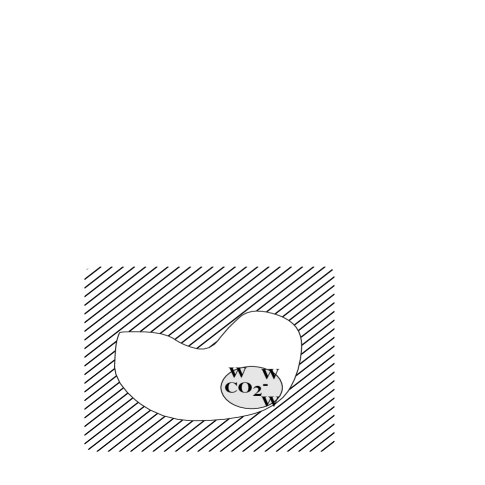
Figure 4: How the quasi-chemical approach might provide an explicit-implicit model of macromolecule hydration. The proximal volume is defined about a hydrophilic (carboxylate) side chain of a protein. The ‘W’s indicate water molecules that might occupy the defined bonding region. The material external to the protein plus ligand complex might be treated by a crude physical model such as a dielectric continuum model appropriate for longer-ranged and weaker interactions.

In these complicated settings, it is worthwhile to notice that the theoretical development can be expressed in a way that is consistent with understood simulation techniques. We consider a specific $n^{th}$ term of the sum of Eq. (34) and then the inner-most average expressed there:

$$s_{\sigma W_{n}}{}^{(0)}({\bf 1+n})p_{0}\left\langle{e^{-\beta\Delta U}}\right\rangle_{0}^{*}z^{n}q_{\sigma W_{n}}=e^{-\beta{\mathcal{F}}_{\sigma W_{n}}({\bf 1+n})}\left({{{z^{n}}\over{n!}}}\right).$$ (44)

This equation introduces the conformational free energy ${\mathcal{F}}_{\sigma W_{n}}({\bf 1+n})$ associated with a geometry of the solute and $n$ specific solvent (water) molecules within the defined proximal volume. The factor $n!$ on the right arises because $n!\,q_{\sigma W_{n}}$ is the normalizing feature of $s_{\sigma W_{n}}{}^{(0)}({\bf 1+n})$ involved in Eq. (30). Our quasi-chemical master formula, Eq. (34), can then be expressed as

$${\rho_{\sigma}\over z_{\sigma}}=V^{-1}\sum\limits_{n\geq 0}{\left({{{z^{n}}\over{n!}}}\right)Tr_{n}\left({e^{-\beta{\mathcal{F}}_{\sigma W_{n}}}}\right)}.$$ (45)

$Tr_{n}\left(\ldots\right)$ indicates the trace as it might appear, for example, in the conventional evaluation of a canonical partition function. That term evaluates to $n!\,q_{\sigma W_{n}}$ — the ‘configuration integral’ hill:config_int for the isolated cluster — in the case that the external-cluster interactions are negligible. The formula Eq. (45) suggests a grand canonical ensemble calculation but with some primitive and essential differences. Firstly, the volume of the system is attached to the solute and, in fact, this volume can change as the solute changes conformation. Secondly, the function appearing where the potential energy would appear is the conformational free energy ${\mathcal{F}}_{\sigma W_{n}}({\bf 1+n})$. This depends on the thermodynamic state of the solvent, that is, on $z$ and $\beta$. When $z$=0, only the n=0 term of Eq. (45) is non-zero and then Eq. (45) is trivially verified with $\beta\Delta\mu_{\sigma}$=0. Finally, the thermodynamic identification of this partition function is the combination on the left side of Eq. (45).

Despite these important differences, the structural similarity of Eq. (45) with a grand canonical partition function is remarkable. Calculations that used this approach would be built upon a model for ${\mathcal{F}}_{\sigma W_{n}}({\bf 1+n})$, which included physical approximations for the extra-cluster contributions, and on the simulation algorithms for calculations on grand canonical ensembles. Grand canonical simulation calculations are less routine than other types of simulations and probably more demanding when applied to condensed phases. If grand canonical simulations were prohibative in a particular case because of a lack of facility of molecule exchange, then these approaches might also be prohibitive because of that. Practical points of difference might help, however. The present development is designed so that the number of ligand molecules needn’t be great. Additionally, the conformational changes of the solute can change the defined proximal volume, changing the local ligand binding characteristics either to squeeze out ligands or to open space for insertion of new ligands.

Again we emphasize the idea that if the proximal volumes are defined to be aggressively small then the evaluation of the partition functions indicated in Eq. (45) should be simpler. In the most favorable case, the indicated partition functions might be evaluated by a maximum term and gaussian distribution procedure. In that case, the computational work to exploit this proposal is only slightly greater than a determination of an optimum hydration structure for the ligands. Roughly put, the theory provides a justification for treating a small set of waters as part of the solute molecule under study. The theory then suggests consideration of the ‘chemical’ reaction for isolated reaction species. According to this approach, the study of the ligands and of the complex, then inclusion of a simple implicit solvent model permits an inference of the basic hydration free energy for the solute alone.

Discussion

In the area of computational theory for aqueous solution chemistry and biochemistry, there seems to be a well developed folklore that judicious inclusion of a pivotal few water molecules is typically the important next step beyond dielectric continuum implicit solvent models. The quasi-chemical approach developed here is the statistical mechanical theory for how to do that properly for solution thermodynamics.

Implicit Solvent Models

One goal of an implicit solvent model is to increase computational scope. Otherwise inaccessible problems might become accessible to study. Or, perhaps, hundreds of instances might be checked with implicit solvent models where only one instance could be examined if sufficient water must be explicitly included. This increased scope is accomplished, in concept at least, by reducing the amount of solvent that must be explicitly tracked in a simulation calculation. The prices to be paid for this reduction are the approximations that must be accepted and the increased complexity of the implicit calculation. How the advantages and complications balance in particular cases typically has been unclear.

Nevertheless, there are other potential advantages of implicit solvent models and the chief of these is the same advantage offered by approximate physical theories. Scientific use of such theories serves to establish simplified concepts that are valid and valuable where the goal is understanding as well as predicting. The physical idea implicit in the developments above is that a handful of proximal water molecules are decisive for chemistry and biochemistry in aqueous solution. Even for such extended molecular events as protein folding, it is a valuable hypothesis that a small number of water molecules, perhaps hundreds rather than a hundred times that, play a decisive role.

The quasi-chemical factors of $\rho_{H_{2}O}{}^{n}$ of Eqs. (1) and (35) are the most basic feature of the environment mean-field operating on the solvent molecules included explicitly. This identification is a basic difference from other implicit solvent models and suggests the possibility of aggressively pushing the numbers of explicitly included solvent molecules down to minimal chemically reasonable values.

Dielectric Models and Electronic Structure Calculations for Solution Thermodynamics

Explicit treatment of water molecules that are near-neighbors of the solutes should mitigateHummer:97c the awkward, not always well-defined invocations of “dielectric saturation and electrostriction.” In this way, quasi-chemical developments also address lingering foundational problems with dielectric models in applications to solution chemistry. Parameterization of dielectric models to describe variations of hydration free energies with temperature, pressure, composition, and solute conformationPratt:94a ; Tawa:94 ; Tawa:95 ; Pratt:97 ; Hummer:98 are as relevant as the foundational issues. For the quasi-chemical models used here, some empirical parameterization is still required for the ligands that form the exterior of the complex. In the Li⁺ example, this means radii parameters are required for the water molecules involved. However, the results are insensitive to radii parameters required for the solute Li⁺ ion; and furthermore, as the theoretical development emphasizes, the product of such efforts is the thermodynamic characteristics of the solute, not the ligands. The development above has emphasized that much of the thermodynamic state dependence of hydration free energies is explicitly available in quasi-chemical approaches.

Similarly, phenomena involving the electronic structure of the solute are naturally, though approximately, included in quasi-chemical theories. Examples of such phenomena are nuclear versus electronic time scale issues, dispersion interactions and electron correlation more generally, the orthogonality or ‘charge-leakage’ issues that are currently discussed for dielectric models, and solute-solvent charge transfer that was observed for the Li⁺ example, see Table 1. They may be excluded in unvarnished dielectric models, or included in only ad hoc ways. Since it is the molecular and thermodynamic properties of the solute that is the goal of the quasi-chemical theories, the phenomena listed above are reasonably included for the solute properties.

Conclusions

This paper has given an extended development of the quasi-chemical approach to computational solution chemistry and biochemistry and discussed the relevance of this development to problems of implicit solvent models of the structural molecular biology. The new implicit solvent model presented here is, more accurately, an explicit-implicit model applicable to the statistical thermodynamics of solutions. The physical idea for the model is that a small subset of solvent molecules are decisive for the statistical thermodynamics and require explicit treatment, whereas the remaining solvent molecules are less important and may be treated implicitly.

The formal derivation of the quasi-chemical formula depends on the well-known potential distribution theorem aided by a clustering analysis that serves as a counting device. In the process of the derivation, it is shown how the view of the system is transformed from a single solute in solution to a solute complexed to solvent ligand molecules interacting with the extra-complex solution. The thermodynamic derivation and the quasi-chemical rule that results, Eq. (41), are new.

To illustrate the quasi-chemical approach, the hydration thermodynamic properties of Li⁺(aq) are calculated. The problem is framed as a series of ion hydration reactions involving the isolated ion, water molecule ligands, and ion-ligand complexes. Application of an implicit solvent model to the species, the standard dielectric continuum model in this case, accounts for interactions with the extra-complex solvent molecules. The results predict that Li⁺ in liquid water is surrounded by four (4) inner shell water molecule ligands with a chemical potential comparable to experimental results. Since the explicit pressure and temperature dependencies of the chemical potential are analytically available in the quasi-chemical formula, results for the partial molar volume and entropy of Li⁺(aq) are explicitly available. The evaluations of the partial molar volume and partial molar entropy of the Li⁺(aq) give a snapshot of the status of molecular theory for these properties.

References

- (1) Berkowitz, M. and McCammon, J. A., Chem. Phys. Letts. 90, 215 (1982).
- (2) Brooks, C. L., and Karplus, M., J. Chem. Phys. 79, 6312 (1983).
- (3) Brunger, A.,Brooks, C. L., and Karplus, M., Chem. Phys. Letts. 105, 495 (1984).
- (4) Belch, A. C., and Berkowitz, M., Chem. Phys. Letts. 113, 278 (1985).
- (5) Brooks, C. L., Brunger, A.,and Karplus, M., Biopolymers 24, 843 (1985).
- (6) Brooks, C. L., and Karplus, M., Meth. Enzym. 127, 369 (1986).
- (7) Pratt, L. R., and Chandler, D., Meth. Enzym. 127, 48 (1986).
- (8) Brunger, A. T., Huber, R., and Karplus, M., Biochem. 26, 5153 (1987).
- (9) Brooks, C. L., and Karplus, M., J. Molec. Bio. 208, 159 (1989).
- (10) Brooks, C. L., III, Karplus, M., and Pettitt, B. M., Adv. Chem. Phys. LXXI, 1 (1988).
- (11) Deloof, H., Harvey, S. C., Segrest, J. P., and Pastor, R. W., Biochem. 30, 2099 (1991).
- (12) Levchuk, V. N., Sheykhet, I., and Simkin, B. Y., Chem. Phys. Letts. 185, 339 (1991).
- (13) Shiratori, Y. and Nakagawa, S., J. Comp. Chem. 12, 717 (1991).
- (14) Straub, J. E., and Karplus, M., Chem. Phys. 158, 221 (1991).
- (15) Braatz, J. A., Paulsen, M. D., and Ornstein, R. L., J. Biomol. Struct. Dyn. 9, 935 (1992).
- (16) Tapia, O., J. Math. Chem. 10, 139 (1992).
- (17) Widmalm, G., and Pastor, R. W., J. Chem. Soc. Faraday Trans. 88, 1747 (1992).
- (18) Heller, H., Schaefer, M., and Schulten, K., J. Phys. Chem. 97, 8343 (1993).
- (19) Fritsch, V., Ravishanker, G., Beveridge, D. L., and Westhof, E., Biopolymers 33, 1537 (1993).
- (20) Juffer, A. H., and Berendsen, H. J. C., Molec. Phys. 79, 623 (1993).
- (21) Nakagawa, S., Yu, H. A., Karplus, M., and Umeyama, H., Prot. Struct. Func. Gene. 16, 172 (1993).
- (22) Rashin, A. A., Prog. Biophys. Molec. Bio. 60, 73 (1993).
- (23) Beglov, D., and Roux, B. J. Chem. Phys. 100, 9050 (1994).
- (24) Arnold, G. E., and Ornstein, R. L., Prot. Struct. Func. Gene. 18, 19 (1994).
- (25) Axelsen, P. H., Harel, M., Silman, I., and Sussman, J. L., Protein Science 3, 188 (1994).
- (26) Davis, M. E., Biophys. J. 66, A290 (1994).
- (27) Lazaridis, T., and Paulaitis, M. E., J. Am. Chem. Soc. 116, 1546 (1994).
- (28) Pastor, R. W., Curr. Op. Struct. Bio. 4, 486 (1994).
- (29) Straub, J. E., Lim, C., and Karplus, M., J. Am. Chem. Soc. 116, 2591 (1994).
- (30) Sharp, K. A., Curr. Op. Struct. Bio. 4, 234 (1994).
- (31) Beglov, D., and Roux, B. Biopolymers 35, 171 (1995).
- (32) Eriksson, M. A. L., and Nilsson, L., J. Molec. Bio. 253, 453 (1995).
- (33) Essex, J. W., and Jorgensen, W. L., J. Comp. Chem. 16, 951 (1995).
- (34) Norberg, J., and Nilsson, L., J. Phys. Chem. 99, 14876 (1995).
- (35) Alaman, C., J. Biomol. Struct. Dyn. 14, 193 (1996).
- (36) Bencsura, A., Enyedy, I. Y., and Kovach, I. M., J. Am. Chem. Soc. 118, 8531 (1996).
- (37) David, L., and Field, M. J., J. Molec. Mod. 2, 427 (1996).
- (38) Larwood, V. L., Howlin, B. J., and Webb, G. A., J. Mol. Mod. 2, 175 (1996).
- (39) Luty, B. A., and van Gunsteren, W. F., J. Phys. Chem. 100, 2581 (1996).
- (40) Wang, L., and Hermans, J., Molec. Sim. 17, 67 (1996).
- (41) Albaret, C., et al., Prot. Struct. Func. Gene. 28, 543 (1997).
- (42) Haggett, N. M. W., Hoffmann, R. A., Howlin, B. J., and Webb, G. A., J. Mol. Mod. 3, 301 (1997).
- (43) Han, J., Jaffe, R. L., and Yoon, D. Y., Macromol. 30, 7245 (1997).
- (44) Meirovitch, H., and Hendrickson, T. F., Prot. Struct. Func. Gene. 29, 127 (1997).
- (45) Parrill, A. L., Mamuya, N., Dolata, D. P., and Gervay, J., Glycoconjugate J. 14, 523 (1997).
- (46) Nadig, G., Van Zant, L. C., Dixon, S. L., and Merz, K. E., J. Am. Chem. Soc. 120, 5593 (1998).
- (47) Zeng, J., Treutlein, H. R., and Simonson, T., Prot. Struct. Func. Gene. 31, 186 (1998).
- (48) Lounnas, V., Ludemann, S. K., and Wade, R. C., Biophys. Chem. 78, 157 (1999).
- (49) Prabhu, N. V. et al., Biophys. Chem. 78, 113 (1999).
- (50) Roux, B.,and Simonson, T., Biophys. Chem. 78, R9 (1999).
- (51) Roux, B. and Simonson, T., Biophys. Chem. 78, 1 (1999).
- (52) Roux, B., Beglov, D., and Im, W., Generalized Solvent Boundary Potential for Computer Simulations, this volume (1999).
- (53) Zhang, L. Y., Gallicchio, E., and Levy, R. M., Implicit Solvent Models for Protein-Ligand Binding: Insights Based on Explicit Solvent Simulations, this volume (1999).
- (54) Marx, D., in New Approaches in Problems in Liquid State Theory, Vol. 529 of NATO Science Series, edited by C. Caccamo, J.-P. Hansen, and G. Stell (Kluwer, Dordrecht, 1999), pp. 439–457.
- (55) Lubin, M. I., Bylaska, E. J., and Weare, J. H., xxx.lanl.gov cond-mat/9905197, (1999).
- (56) Guggenheim, E. A., Proc. Rov. Soc. London A 148, 304 (1935).
- (57) Bethe, H., Proc. Rov. Soc. London A 150, 552 (1935).
- (58) Brush, S. G., and Kikuchi, R., Technical Report No. UCRL-14287, University of California, Lawrence Radiation Laboratory, Livermore, California (unpublished).
- (59) Martin, R. L., Hay, P. J., and Pratt, L. R., J. Phys. Chem. A 102, 3565 (1998).
- (60) Rempe, S. B. et al., Technical Report No. LA-UR-99-3360, Los Alamos National Laboratory (unpublished).
- (61) Foresman, J. B., and Frisch, Æ., Exploring Chemistry with Electronic Structure Methods (Gaussian, Inc., Pittsburgh, PA 15106, 1996).
- (62) Stefanovich, E. V., and Truong, T. N., Chem. Phys. Lett. 244, 65 (1995).
- (63) Frisch, M. J. et al., Gaussian 98 (Revision A.2) (Gaussian, Inc., Pittsburgh PA, 1998).
- (64) Pratt, L. R., Hummer, G., and Garde, S., in New Approaches in Problems in Liquid State Theory, Vol. 529 of NATO Science Series, edited by C. Caccamo, J.-P. Hansen, and G. Stell (Kluwer, Dordrecht, 1999), pp. 407–420.
- (65) McQuarrie, D. A., in Statistical Mechanics (Harper & Row, New York, 1976), see Chapter 9.
- (66) Marcus, Y., Biophys. Chem. 51, 111 (1994).
- (67) Friedman, H. L., and Krishnan, C. V., in Water A Comprehensive Treatise, edited by F. Franks (Plenum Press, New York, 1973), Vol. 3, pp. 1–118.
- (68) Pratt, L. R., and LaViolette, R. A., Mol. Phys. 94, 909 (1998).
- (69) Pratt, L. R., Hummer, G., and García, A. E., Biophys. Chem. 51, 147 (1994).
- (70) Tawa, G. J., and Pratt, L. R., in Structure and Reactivity in Aqueous Solution. Characterization of Chemical and Biological Systems, Vol. 568 of ACS SYMPOSIUM SERIES, edited by C. J. Cramer and D. G. Truhlar (American Chemical Society, Washington DC, 1994), pp. 60–70.
- (71) Tawa, G. J., and Pratt, L. R., J. Am. Chem. Soc. 117, 1625 (1995).
- (72) Pratt, L. R. et al., Int. J. Quant. Chem. 64, 121 (1997).
- (73) Hummer, G., Pratt, L. R., and García, A. E. J. Phys. Chem. A 102, 7885 (1998).
- (74) Floriano, W. B., Nascimento, M. A. C., Domont, G. B., and Goddard, W. A., Protein Science 7, 2301 (1998).
- (75) Pratt, L. R., and Pohorille, A., in Proceedings of the EBSA 1992 International Workshop on Water-Biomolecule Interactions, edited by M. U. Palma, M. B. Palma-Vittorelli, and F. Parak (Societa Italiana di Fisica, Bologna, 1993), pp. 261–268.
- (76) Matubayasi, N., Reed, L. H., and Levy, R. M., J. Phys. Chem. 98, 10640 (1994).
- (77) Matubayasi, N., and Levy, R. M., J. Phys. Chem. 100, 2681 (1996).
- (78) Clever, H. L., in Solubility Data Series (Pergamon Press, Oxford, 1979), Vol. 1, p. 4.
- (79) Heinzinger, K., and Pálinkás, G., in The Chemical Physics of Solvation, edited by R. R. Dogonadze (Elsevier, Amsterdam, 1985), Vol. 38a, p. 313.
- (80) Mezei, M., and Beveridge, D. L., J. Chem. Phys. 74, 6902 (1981).
- (81) Impey, R. W., Madden, P. A., and McDonald, I. R., J. Phys. Chem. 87, 5071 (1983).
- (82) Chandrasekhar, J., Spellmeyer, D. C., and Jorgensen, W. L., J. Am. Chem. Soc. 106, 903 (1984).
- (83) Bounds, D. G., Mol. Phys. 54, 1335 (1985).
- (84) Zhu, S. B., and Robinson, G. W., Z. Naturforsch. A 46, 221 (1991).
- (85) Romero, C., J. Chim. Phys. 88, 765 (1991).
- (86) Lee, S. H., and Rasaiah, J. C., J. Chem. Phys. 101, 6964 (1994).
- (87) Toth, G., J. Chem. Phys. 105, 5518 (1996).
- (88) Koneshan, S., Rasaiah, J. C., Lynden-Bell, R. M., and Lee, S. H., J. Phys. Chem. B 102, 4193 (1998).
- (89) Haar, L., Gallagher, J. S., and Kell, G. S., NBS/NRC Steam Tables (Hemisphere Publishing Company, New York, 1984).
- (90) Garde, S., et al., Phys. Rev. Letts. 77, 4966 (1996).
- (91) Widom, B., J. Phys. Chem. 86, 869 (1982).
- (92) Pratt, L. R., in Encyclopedia of Computational Chemistry, edited by Schleyer, P. v. R., et al. (John Wiley & Sons, Chichester, 1998), pp. 1286–1294.
- (93) Uhlenbeck, G. E., and Ford, G. W., in Lectures in Applied Mathematics (American Mathematical Society, Providence, RI, USA, 1963), Vol. I, pp. 36–38.
- (94) van Kampen, N. G., in Stochastic Processes in Physics and Chemistry, revised and enlarged ed. (North Holland, Amsterdam, 1992), page 31.
- (95) Feynman, R. P., in Statistical Mechanics (W. A. Benjamin, Inc., Reading, Massachusetts, 1972), Chap. 5. Order-disorder Theory.
- (96) Hummer, G., et al., Proc. Nat. Acad. Sci. USA 93, 8951 (1996).
- (97) Hummer, G., et al., Proc. Natl. Acad. Sci. USA 95, 1552 (1998).
- (98) Hummer, G., et al., J. Phys. Chem. B 102, 10469 (1998).
- (99) Gomez, M. A., Pratt, L. R., Hummer, G., and Garde, S., J. Phys. Chem. B 103, 3520 (1999).
- (100) Garde, S., García, A. E. Pratt, L. R., and Hummer, G., Biophys. Chem. 78, 21 (1999).
- (101) Hill, T. L., in Statistical Mechanics (Dover, New York, 1956), see section 22.
- (102) Hummer, G., Pratt, L. R., and García, A. E., J. Am. Chem. Soc. 119, 8523 (1997).