Extended Gaussian wave packet dynamics

Abstract

We examine an extension to the theory of Gaussian wave packet dynamics in a one-dimensional potential by means of a sequence of time dependent displacement and squeezing transformations. Exact expressions for the quantum dynamics are found, and relationships are explored between the squeezed system, Gaussian wave packet dynamics, the time dependent harmonic oscillator, and wave packet dynamics in a Gauss-Hermite basis. Expressions are given for the matrix elements of the potential in some simple cases. Several examples are given, including the propagation of a non-Gaussian initial state in a Morse potential.

I Introduction

Wave packet dynamics has exposed interesting new phenomena in several fields. In femto-chemistry [1, 2] we are now able to time-resolve chemical processes and also observe effects such as the breakup and revival of wave packets [3]. In atom optics wave packets are used to model matter waves [4], and electron wave packets are seen in the dynamics of Rydberg atoms [5]. The numerical modelling of wave packet dynamics has been achieved by a number of methods [6, 2], but one of the earliest approaches was by Heller [7] who simply used the Ansatz of a time dependent Gaussian wave packet. This Gaussian approach is very useful, but it is usually an approximation and can be quite wrong, for example at turning points. Several improvements have been made: for example, the method of generalised Gaussian wave packets [8] used complex classical trajectories for Gaussian wave packets, and the hybrid method [9] used an expansion in terms of a grid of Gaussian wave packets.

The idea of using a time dependent harmonic (i.e. Gauss-Hermite) basis, in the context of wave packet propagation, was put forward by Lee and Heller [10] and Coalson and Karplus [11]. The basis was chosen so that the lowest eigenstate matches the Heller Gaussian wave packet, but with the inclusion of a complete set of basis states the modelling can be performed accurately. This approach was generalised to multi-dimensional systems by Lee [12]. However, several possibilities for using a Gauss-Hermite basis exist: parameters for the dynamic basis were treated in a variational method by Kay [13] and by Kucar and Meyer [14], more recently the phase space picture was explored by Møller and Henriksen [15], and the use of a Gauss-Hermite basis with a variational treatment has been expanded by Billing [16, 17, 18] to examine non-adiabatic transitions and corrections to classical path equations.

The approach that is used in this paper is similar, in principle, to the time dependent Gauss-Hermite basis of Refs. [10] and [11]; in each case the basis follows the Heller Gaussian wave packet. However, the focus here is on the evolution operator and transformations associated with the time-dependent basis which becomes both “displaced” and “squeezed”. That is, unlike previous extensions to Gaussian wave packet dynamics, the system Hamiltonian is transformed by displacement and squeezing in a way that removes all operator dependence which is quadratic or less. The result is an evolution equation which depends on a time dependent ‘residual potential’ which is based on the original (one-dimensional) potential with harmonic terms removed. This means that if the higher order derivatives of the potential are small, the system evolution will change relatively slowly, which allows a rapid numerical integration (of a set of ordinary differential equations). The method, which is in principle exact, is then similar to a time-dependent perturbation theory in a time dependent basis or interaction picture. Indeed, it can be developed as a perturbation theory in the higher order derivatives of the system potential about the classical motion.

Because the evolution operator is found, the possibility exists for applying this extended Gaussian wave packet method to initial states that are not Gaussian. The evolution operator also allows us to use the displacement and squeezing transformations to find explicit matrix elements of the residual potential using standard operator algebra.

In section II of this paper we set up the problem and perform a basis shift according to the classical dynamics. Section III examines Gaussian wave packet dynamics in this displaced basis, and in the original basis by two different approaches. The relationship between the two approaches is established. In section IV we establish the squeezing transformation necessary to map the time evolution of a Gaussian wave packet from its initial state. By using the same transformation for another change of basis we can find the equations for corrections to Gaussian wave packet dynamics. These equations are expressed in a Fock basis in section V, where we also compare our results to the Gauss-Hermite basis. Some examples of useful matrix elements for potentials are given in section VI, and in section VII the results are applied to several different problems.

II Displaced basis

A Scaling of the problem

The problem we wish to describe is the one dimensional problem of a wave packet in a potential described by the Hamiltonian

$${\widetilde{H}}=\frac{{\widetilde{p}}^{2}}{2m}+{\widetilde{U}}({\widetilde{x}})\;.$$ (1)

The position and momentum co-ordinates have been denoted by ${\widetilde{x}}$ and ${\widetilde{p}}$ to distinguish them from scaled quantities that will shortly be introduced. The initial wave packet will be taken to be a Gaussian one. This is not essential, but it will simplify the treatment that will follow. The key feature is that a length scale, characteristic of the initial wave packet defines the width of the harmonic oscillator basis that we will use. For a Gaussian initial wave packet

$$\Psi_{0}({\widetilde{x}})=\frac{1}{(2\pi\sigma_{0}^{2})^{1/4}}\exp\left[-\frac{({\widetilde{x}}-{\widetilde{x}}_{0})^{2}}{4\sigma_{0}^{2}}+i\frac{{\widetilde{p}}_{0}{\widetilde{x}}}{\hbar}\right]\;,$$ (2)

which has a width $\sigma_{0}$ and is located at ${\widetilde{x}}_{0}$ with momentum ${\widetilde{p}}_{0}$.

We will now adopt a scaling of the problem such that we use the operators

$$\hat{x}=\frac{{\widetilde{x}}}{\sqrt{2}\sigma_{0}}$$ (3)

$$\hat{p}=\frac{\sqrt{2}\sigma_{0}{\widetilde{p}}}{\hbar}$$ (4)

which have the commutator $[\hat{x},\hat{p}]=i$. The Schrödinger equation then reduces to

$$i\frac{\partial\Psi}{\partial t}=\left[\frac{\hat{p}^{2}}{2}+U(\hat{x})\right]\Psi\;,$$ (5)

where we use scaled time and energy,

$$t={\widetilde{\omega}}_{0}{\widetilde{t}}$$ (6)

$$U={\widetilde{U}}/(\hbar{\widetilde{\omega}}_{0})\;.$$ (7)

The frequency ${\widetilde{\omega}}_{0}$ is determined by the width of the initial wave packet. It is the frequency of the harmonic oscillator for which the wave function (2) is a ground state wave function,

$${\widetilde{\omega}}_{0}=\frac{\hbar}{2m\sigma_{0}^{2}}\;.$$ (8)

In terms of the scaled quantities the initial wave function is now

$$\Psi_{0}(x)=\frac{1}{\pi^{1/4}}\exp\left[-\frac{(x-x_{0})^{2}}{2}+ip_{0}x\right]\;,$$ (9)

when we use the appropriately scaled $x_{0}$ and $p_{0}$.

B Local expansion of the potential

The motion of a Gaussian wave packet in a harmonic potential is exactly solvable, even when the potential is time dependent, and we will use this to define the local basis for the wave packet. That is, the potential function $U(x)$ will be expanded to second order about the the position of the wave packet. The dynamics of a Gaussian wave packet in this harmonic potential will be determined, and these dynamics will be used to define the basis for the full (non-Gaussian) wave packet dynamics.

The wave packet (9) is located at the position $x_{0}$, which will in general be time dependent; we then take its location to be given by $x_{0}(t)$. If we expand the potential about this point we obtain,

$$U(x)=U(x_{0})+U^{\prime}(x_{0})(x-x_{0})+\frac{U^{\prime\prime}(x_{0})}{2}(x-x_{0})^{2}+U_{R}(x,x_{0})\;,$$ (10)

where the spatial derivatives are indicated with the primes. The terms in the expansion are not explicitly time dependent; they vary only with time through the position $x_{0}(t)$. The potential function $U_{R}(x,x_{0})$ is the residual potential found after making the harmonic expansion. That is, it contains the higher order, cubic and above, terms in the expansion. The residual potential will play a central role in the non-Gaussian dynamics of the wave packet, and Eq. (10) serves as its definition.

C Displacement of the basis

In the following, we will make two basis changes in order to match the Gaussian part of the wave packet dynamics. The first basis transformation will be a displacement to remove the linear term in $x$ from the potential in Eq. (10). The necessary displacement is simply $x_{0}(t)$ in space and a momentum $p_{0}(t)$, such that the wave function is shifted to the origin. The new wave function will be

$$\psi_{d}(x,t)=\hat{D}(-\beta(t))\Psi(x,t)\;,$$ (11)

i.e. $\Psi(x,t)=\hat{D}(\beta(t))\psi_{d}(x,t)$, where $\hat{D}(\beta(t))$ is the time dependent displacement operator

$$\hat{D}(\beta(t))=\hat{D}^{-1}(-\beta(t))=\exp\left(ip_{0}(t)\hat{x}-ix_{0}(t)\hat{p}\right)\;,$$ (12)

with

$$\beta=\frac{x_{0}+ip_{0}}{\sqrt{2}}\;.$$ (13)

The potential $U(x)$ in the Schrödinger equation (5) will become transformed as $D^{-1}(\beta(t))U(\hat{x})\hat{D}(\beta(t))=U(x_{0}+\hat{x})$ and we will then use the expansion in Eq. (10).

The requirement to remove the linear $\hat{x}$ term (and linear $\hat{p}$ term) from the potential means that after inserting Eq. (11) in the Schrödinger equation (5) we obtain the conditions:

$$x_{0}^{\prime} = p_{0}(t)$$ (14)

$$p_{0}^{\prime} = -U^{\prime}(x_{0}(t))$$ (15)

which are, of course, the classical equations of motion. With these conditions the linear term in $\hat{x}$ is lost and the Schrödinger equation now reads

$$i\frac{\partial\psi_{d}(x,t)}{\partial t}=\left[\frac{\hat{p}^{2}}{2}+U(x_{0}(t))-\frac{1}{2}U^{\prime}(x_{0}(t))x_{0}(t)+\frac{U^{\prime\prime}(x_{0}(t))}{2}\hat{x}^{2}+U_{R}(x_{0}+\hat{x},x_{0})\right]\psi_{d}(x,t)\;.$$ (16)

The non-operator parts of Eq. (16) are easily removed with a time dependent phase factor

$$\phi_{U}(t)=\int^{t}\left[U(x_{0}(t^{\prime}))-\frac{1}{2}x_{0}(t^{\prime})U^{\prime}(x_{0}(t^{\prime}))\right]dt^{\prime}=\int^{t}\left[\frac{1}{2}x_{0}(t^{\prime})p^{\prime}_{0}(t^{\prime})+U(x_{0}(t^{\prime}))\right]dt^{\prime}\;,$$ (17)

where for the second form we have used Eq. (15). Then if we define the displaced wave function with a phase shift as

$$\psi_{dp}(x,t)=e^{i\phi_{U}(t)}\psi_{d}(x,t)=e^{i\phi_{U}(t)}\hat{D}(-\beta(t))\Psi(x,t)\;,$$ (18)

we obtain the Schrödinger equation

$$i\frac{\partial\psi_{dp}(x,t)}{\partial t}=\left[\frac{\hat{p}^{2}}{2}+\frac{U^{\prime\prime}(x_{0}(t))}{2}\hat{x}^{2}+U_{R}(x_{0}+\hat{x},x_{0})\right]\psi_{dp}(x,t)\;.$$ (19)

Basis displacement has been of interest in the study of quantum state diffusion (QSD) [19] where the non-linear dynamics create wave packet localisation. By using a displaced basis a reduction in computational effort is gained. However, in quantum state diffusion there is no strong motive for going to the next step of squeezing the basis because QSD localised wave packets all have the same size. In ordinary Schrödinger wave packet dynamics wave packets can change their widths enormously making basis squeezing desirable.

III Gaussian wave packet dynamics

A Heller’s approach

For completeness we include here an outline of standard Gaussian wave packet dynamics. Heller started with the Ansatz [7]

$$\Psi_{GWP}=\exp\left[i\alpha(t)(x-x_{0}(t))^{2}+ip_{0}(t)(x-x_{0}(t))+i\gamma(t)\right]$$ (20)

in the original basis [here we use the scaled basis of Eq. (4)]. The normalisation is included in the time dependent complex parameter $\gamma(t)$, and Heller introduced the parameter $\alpha(t)$ which characterises (the reciprocal of) the width of the Gaussian wave packet. The position $x_{0}$ and momentum $p_{0}$ of the wave packet obey the classical equations of motion, exactly as in Eqs. (14) and (15). By substituting the Gaussian wave packet into the Schrödinger equation (5) with the truncated potential

$$U(x)\sim U(x_{0})+U^{\prime}(x_{0})(x-x_{0})+\frac{U^{\prime\prime}(x_{0})}{2}(x-x_{0})^{2}\;,$$ (21)

we can show that

$$\alpha^{\prime} = -2\alpha^{2}-U^{\prime\prime}(x_{0})/2$$ (22)

$$\gamma^{\prime} = i\alpha+p_{0}x_{0}^{\prime}-E$$ (23)

where $E$ is the classical energy $p_{0}^{2}/2+U(x_{0})$.

Thus the dynamics of an approximate Gaussian wave packet are completely defined by solving the differential equations (14), (15), and (23). The result is approximate because Eq. (21) is an approximation to Eq. (10).

B Gaussian wave packets in the displaced basis

In order to establish some notation, and motivate the squeezing transformation in section IV, this section gives an overview of Gaussian wave packet dynamics as found in the displaced basis of Eq. (11). Thus starting with Eq. (19), we again neglect the residual potential $U_{R}$ to obtain

$$i\frac{\partial\psi_{s}(x,t)}{\partial t}=\left[\frac{\hat{p}^{2}}{2}+\frac{k(t)}{2}\hat{x}^{2}\right]\psi_{s}(x,t)\;,$$ (24)

where $k(t)=U^{\prime\prime}(x_{0}(t))$ is a time dependent spring constant. This Schrödinger problem does have a known time dependent ‘ground’ state solution (see, for example, Ref. [20]), which is not a stationary state, because of the time dependence in $k(t)$. The ‘ground’ state solution can be formulated in terms of local classical trajectories. Using some of the notation of Ref. [20] we define a quantity $\epsilon(t)$, through the equation

$$\epsilon^{\prime\prime}(t)=-k(t)\epsilon(t)\;,$$ (25)

which would make $\epsilon$ follow the classical trajectory of a point close to the centre of the wave packet. For $\epsilon$ we have the following, complex, initial conditions

$$\epsilon(0) = 1$$ (26)

$$\epsilon^{\prime}(0) = i$$ (27)

so that we have a time independent Wronskian with the value

$${\cal W}=\epsilon^{\prime}\epsilon^{\ast}-\epsilon\epsilon^{\prime}\!\,{}^{\ast}=2i\;.$$ (28)

Then the ground state wave function takes the form [20]

$$\psi_{s}(x,t)=\frac{1}{\pi^{1/4}\sqrt{\epsilon(t)}}\exp\left[\frac{i\epsilon^{\prime}(t)}{2\epsilon(t)}x^{2}\right]\;,$$ (29)

as may be verified by substitution into Eq. (24). We note that the time dependent width of this wave packet is $1/\surd[2$Im$(\epsilon^{\prime}/\epsilon)]$ which is found to be $|\epsilon|/\sqrt{2}$ on using the Wronskian (28). The ground state wave function (29) is identical to the Heller Gaussian wave packet if we transform it back to the original basis using the inverse of Eq. (18). That is,

$$\Psi_{GWP}=e^{-i\phi_{U}(t)}\hat{D}(\beta(t))\psi_{s}(x,t)\;.$$ (30)

If we perform the displacement of the wave packet we obtain Eq. (20) with the identifications:

$$\alpha(t) = \epsilon^{\prime}(t)/[2\epsilon(t)]$$ (31)

$$\gamma(t) = x_{0}p_{0}/2-\phi_{U}(t)+g_{n}$$ (32)

where $g_{n}$ is a complex term arising from the normalisation of Eq. (29), i.e.

$$\exp(-ig_{n})=\pi^{1/4}\sqrt{\epsilon(t)}\;.$$ (33)

Thus we see that the Heller Gaussian wave packet corresponds to the evolution of the ‘ground’ state of the time dependent harmonic oscillator (24).

IV Time dependent squeezed basis

In order to go beyond the Gaussian wave packet approximation we need to take into account the non-Gaussian behaviour introduced by the residual potential $U_{R}$. This could, of course, be achieved in any reasonable basis, but in order to take advantage of the power of Gaussian wave packet dynamics, which is often such a good approximation to the time evolution, it makes sense to use a time dependent basis which matches the Gaussian wave packet. To find this basis it is not enough to use the displaced basis of section II C; we must also squeeze the basis to match the (time dependent) width of the Gaussian wave packet as well as its location. Thus, in the same way that we use a displacement operator to remove the linear dependence of the Hamiltonian on $\hat{x}$ in section II C, we will here use a squeezing transformation to remove all quadratic ($\hat{x}$ and $\hat{p}$) terms from the Hamiltonian, thereby leaving the naked dependence on the residual potential $U_{R}$. This will ensure that in the special case where the residual potential is zero, $U_{R}=0$, the transformed wave function is stationary. In this case the displacement and squeezing transformations will map an initial Gaussian wave packet onto Heller’s moving Gaussian wave packet (20). To remove the quadratic operator dependence we denote the squeezing transformation as $\hat{U}_{s}$ and define a wave function $\psi_{sdp}$ in the squeezed and displaced basis as

$$\psi_{sdp}(x,t)=\hat{U}_{s}^{-1}\psi_{dp}(x,t)=\hat{U}_{s}^{-1}e^{i\phi_{U}(t)}\psi_{d}(x,t)=\hat{U}_{s}^{-1}e^{i\phi_{U}(t)}\hat{D}^{-1}(\beta(t))\Psi(x,t)\;.$$ (34)

Writing Eq. (19) as

$$i\frac{\partial\psi_{dp}(x,t)}{\partial t}=\left[H_{s}(t)+U_{R}(x_{0}+\hat{x},x_{0})\right]\psi_{dp}(x,t)\;,$$ (35)

we may substitute for $\psi_{dp}$ from Eq. (34) to obtain

$$i\hat{U}_{s}^{-1}\frac{\partial\hat{U}_{s}}{\partial t}\psi_{sdp}+i\frac{\partial\psi_{sdp}}{\partial t}=\hat{U}_{s}^{-1}\left[H_{s}+U_{R}(x_{0}+\hat{x},x_{0})\right]\hat{U}_{s}\psi_{sdp}\;.$$ (36)

The term $H_{s}$ contains all the quadratic operator dependence and can be removed if the operator $\hat{U}_{s}$ obeys

$$i\hat{U}_{s}^{-1}\frac{\partial\hat{U}_{s}}{\partial t}=\hat{U}_{s}^{-1}H_{s}\hat{U}_{s}\;.$$ (37)

To determine $\hat{U}_{s}$ we will start in the basis of the displaced harmonic oscillator, using the annihilation and creation operators

$$\hat{a} = \frac{\hat{x}+i\hat{p}}{\sqrt{2}}$$ (38)

$$\hat{a}^{\dagger} = \frac{\hat{x}-i\hat{p}}{\sqrt{2}}$$ (39)

so that the Hamiltonian of Eq. (24) [$H_{s}$ in Eq. (35)] becomes

$$H_{s}=\frac{1}{4\epsilon}\left[2(\epsilon-\epsilon^{\prime\prime})\hat{N}-(\epsilon+\epsilon^{\prime\prime})(\hat{a}^{2}+\hat{a}^{\dagger 2})\right]\;,$$ (40)

where

$$\hat{N}=\frac{\hat{a}^{\dagger}\hat{a}+\hat{a}\hat{a}^{\dagger}}{2}=\hat{a}^{\dagger}\hat{a}+1/2\;.$$ (41)

After some consideration we express the unitary operator $\hat{U}_{s}$ in the form

$$\hat{U}_{s}=\hat{S}(\xi)e^{-i\hat{N}\theta}\;,$$ (42)

where $\hat{S}(\xi)$ is the usual squeezing operator [21]

$$\hat{S}(\xi)=\exp\left(-\frac{\xi}{2}\hat{a}^{\dagger 2}+\frac{\xi^{\ast}}{2}\hat{a}^{2}\right)\;.$$ (43)

Then using the standard expressions for the action of the squeeze operator [21], and the phase shifting properties of $e^{-i\hat{N}\theta}$, the operator $\hat{U}_{s}$ will transform the annihilation and creation operators as

$$\hat{U}_{s}^{-1}\hat{a}\hat{U}_{s} = \hat{a}e^{-i\theta}\cosh r-\hat{a}^{\dagger}e^{i(\phi+\theta)}\sinh r$$ (44)

$$\hat{U}_{s}^{-1}\hat{a}^{\dagger}\hat{U}_{s} = \hat{a}^{\dagger}e^{i\theta}\cosh r-\hat{a}e^{-i(\phi+\theta)}\sinh r$$ (45)

where

$$\xi=re^{i\phi}\;.$$ (46)

Explicit expressions for $r$, $\phi$, and $\theta$, will be found by substitution in Eq. (37). However, to determine $\hat{U}_{s}^{-1}\frac{\partial\hat{U}_{s}}{\partial t}$ in Eq. (37) from the Ansatz (42) we need to differentiate the exponential operator $\hat{S}$ with respect to the time dependence of its parameters. This is accomplished by first disentangling the operator, i.e. by using the relation [22]

$$\hat{S}(\xi)=\exp\left(-\frac{1}{2}e^{i\phi}\tanh r\hat{a}^{\dagger 2}\right)\exp\left[-\ln(\cosh r)\hat{N}\right]\exp\left(\frac{1}{2}e^{-i\phi}\tanh r\hat{a}^{2}\right)$$ (47)

and then differentiating. It is then necessary to pull the non-exponential factors containing $\hat{a}$ and $\hat{a}^{\dagger}$ to one side, and re-entangle the squeeze operator before a comparison can be made between both sides of Eq. (37). Some details of this calculation are presented in Appendix A. The final results for the squeezing, and phase, parameters are

$$\tanh r=\frac{\left|\epsilon+i\epsilon^{\prime}\right|}{\left|\epsilon-i\epsilon^{\prime}\right|}$$ (48)

$$e^{i\phi}=-\frac{(\epsilon+i\epsilon^{\prime})}{\left|\epsilon+i\epsilon^{\prime}\right|}\frac{\left|\epsilon-i\epsilon^{\prime}\right|}{(\epsilon-i\epsilon^{\prime})}$$ (49)

$$e^{i\theta}=\frac{(\epsilon-i\epsilon^{\prime})}{\left|\epsilon-i\epsilon^{\prime}\right|}\;.$$ (50)

A few additional relations between $r,\phi$, and $\theta$ can be found in Appendix A.

In this way Eq. (37) is solved and we are left with the residual potential $U_{R}(x_{0}+\hat{x},x_{0})$ in Eq. (36). Because $U_{R}(x_{0}+\hat{x},x_{0})$ depends on the operator $\hat{x}$ it will be transformed under the squeezing transformation (42). Simply by using Eq. (39) with Eq. (45) we find that

$$\hat{U}_{s}^{-1}\hat{x}\hat{U}_{s}=\mbox{Re}[\epsilon(t)]\hat{x}+\mbox{Im}[\epsilon(t)]\hat{p}\;.$$ (51)

Then we obtain from Eq. (36) the “Schrödinger equation”

$$i\frac{\partial\psi_{sdp}}{\partial t}(x,t)=U_{R}\left(x_{0}+\mbox{Re}[\epsilon(t)]\hat{x}+\mbox{Im}[\epsilon(t)]\hat{p}\;,\;x_{0}\right)\psi_{sdp}(x,t)\;,$$ (52)

which is one of our key results. It describes the evolution of a wave function entirely in terms of a “potential” with higher than quadratic behaviour, i.e. in terms of the residual potential $U_{R}$.

We note that neglect of $U_{R}$ in Eq. (52) returns us to Gaussian wave packet dynamics. In this case $\psi_{sdp}$ is stationary and we thus find from Eq. (34) that

$$\Psi_{GWP}(x,t)=e^{-i\phi_{U}(t)}\hat{D}(\beta(t))\hat{U}_{s}(t)\hat{U}_{s}^{-1}(0)\hat{D}^{-1}(\beta(0))\Psi(x,t=0)\;.$$ (53)

This expresses the Heller Gaussian wave packet in terms of a sequence of displacement and squeezing transformations, and would allow us, for example, to propagate a non-Gaussian wave packet in the same way as the Heller Gaussian wave packet is propagated in time.

V Fock state implementation

Our result so far, Eq. (52), describes corrections to Gaussian wave packet dynamics, but is hard to implement because of the appearance of the operator $\hat{p}$ throughout the transformed $U_{R}$. However, it is amenable to treatment in a Fock basis. If we return to the operators $\hat{a}$ and $\hat{a}^{\dagger}$ in Eq. (39) we can write

$$\hat{U}_{s}^{-1}\hat{x}\hat{U}_{s}=\frac{\epsilon^{\ast}(t)\hat{a}+\epsilon(t)\hat{a}^{\dagger}}{\sqrt{2}}\;,$$ (54)

so that the Eq. (52) becomes

$$i\frac{\partial\psi_{sdp}}{\partial t}(x,t)=U_{R}\left(x_{0}(t)+\frac{\epsilon^{\ast}(t)\hat{a}+\epsilon(t)\hat{a}^{\dagger}}{\sqrt{2}}\;,\;x_{0}(t)\right)\psi_{sdp}(x,t)\;.$$ (55)

If we now solve Eq. (55) in a Fock basis we obtain the non-Gaussian wave packet dynamics, i.e. the extended Gaussian wave packet, in the basis defined by the motion of the Gaussian part of the wave packet. To do this we expand the wave function in the Fock basis (of states labelled $|n\rangle$), defined by the Gaussian wave packet ground state

$$\psi_{sdp}(x,t)=\sum_{n}a_{n}(t)|n\rangle\;.$$ (56)

Then the equation of motion becomes

$$i\frac{\partial a_{n}(t)}{\partial t}=\sum_{m}\left\langle n\left|U_{R}\left(x_{0}+\frac{\epsilon^{\ast}\hat{a}+\epsilon\hat{a}^{\dagger}}{\sqrt{2}}\;,\;x_{0}\right)\right|m\right\rangle a_{m}(t)\;.$$ (57)

The equations which have now to be solved depend on the form of $U_{R}$ and its matrix elements. In section VI we will look at some specific functional forms for the residual potential in order to determine explicit expressions for Eq. (57) when matrix elements are taken.

To determine the spatial wave function in the original (scaled) basis and in terms of the coefficients $a_{n}$ we need to express Eq. (56) in the original spatial basis by using the transformation (34). That is, using also Eq. (42),

$$\Psi(x,t)=e^{-i\phi_{U}(t)}\sum_{n=0}^{\infty}a_{n}e^{-i(n+1/2)\theta}\left\langle x\left|\hat{D}(\beta(t))\hat{S}(\xi)\right|n\right\rangle\;.$$ (58)

We then utilize the spatial distribution of squeezed displaced Fock states [23] and after some calculation obtain

$$\Psi(x,t)= \frac{1}{\pi^{1/4}\sqrt{\epsilon}}\exp\left\{i\left[\frac{\epsilon^{\prime}}{2\epsilon}(x-x_{0})^{2}+xp_{0}-x_{0}p_{0}/2-\phi_{U}(t)\right]\right\}$$ (60)

$$\times\sum_{n=0}^{\infty}a_{n}\left(\frac{|\epsilon|}{\sqrt{2}\epsilon}\right)^{n}\frac{1}{\sqrt{n!}}H_{n}\left(\frac{x-x_{0}}{|\epsilon|}\right)\;.$$

The values of $x_{0}(t),p_{0}(t),\epsilon(t),\epsilon^{\prime}(t)$ and $a_{n}(t)$ can be used to determine the spatial wave function. This result for $\Psi$ can be compared to the Ansatz employed as the starting point of the analysis used in Refs. [10, 11, 13, 14, 17], which each use a Gauss-Hermite basis. Refs. [13, 14, 17] all use a variational method where the parameters of the basis depend on the wave function. Refs. [10, 11] use a basis similar to Eq. (60), but since they chose the simplest kind of basis related to the Heller Gaussian wave packet (20) for $n=0$, the expansion used differs from Eq. (60) by phase factors. The $n$th term in Eq. (60) has an additional phase of $(|\epsilon|/\epsilon)^{n}$. Similar phase factors, are absent in variational treatments, for example from Billing’s Ansatz [17] (see also Appendix B). The $n$ dependence of this phase factor means that some quadratic operator dependence is still present in the equations for the amplitudes of the $n$th Fock state. However, the variational methods try to optimise the wave packet trajectory—a process we do not consider here which may compensate. Also note that while Eq. (57) requires the evaluation of matrix elements of the residual potential, similar matrix elements for the full potential are required in Ref. [17]. Again, some analytical approaches to these matrix elements are given in section VI.

Finally, we expect to perform a numerical integration of the various equations to determine the wave packet dynamics of our particular system. The equations which have to be numerically integrated are: (i) the classical equations of motion Eqs. (14), (15), (ii) the $\epsilon$ equation (25), which may be split into two complex first order differential equations, or four real first order equations, and (iii) the amplitudes of the corrections in Eqs. (57). For a basis size of $N$ states, including the lowest energy state, this amounts to $6+2N$ real, first order, linear differential equations. The initial conditions are specified by the initial position and momentum of the wave packet, the initial conditions for $\epsilon$ [Eq. (27)], and, in the case of a Gaussian initial wave packet, $a_{0}=1,a_{n\neq 0}=0$. Then once the various matrix elements in Eq. (57) have been set up, typically involving some finite sums (see the next section), the numerical integration can be done in a straightforward way. Note that, unlike Ref. [10], it is not necessary to use finite difference methods on nearby trajectories, which can result in a reduction of numerical effort.

VI Matrix elements of the residual potential

A Exponential terms in $U_{R}$

We consider a term in $U_{R}$ of the form

$$U_{\beta}(x)=\exp(-\beta_{U}x)\;,$$ (61)

where $\beta_{U}$ is a constant characterising the potential. This term might arise from consideration of a Morse potential and in that case there would be two exponential terms like this one (see Section VII B). Then, following Eq. (55), we will need to evaluate

$$U_{\beta nm}=\left\langle n\left|U_{\beta}\left(\frac{\epsilon^{\ast}(t)\hat{a}+\epsilon(t)\hat{a}^{\dagger}}{\sqrt{2}}\right)\right|m\right\rangle=\left\langle n\left|\exp\left[-\beta_{U}\frac{\epsilon^{\ast}(t)\hat{a}+\epsilon(t)\hat{a}^{\dagger}}{\sqrt{2}}\right]\right|m\right\rangle\;.$$ (62)

We start by disentangling the operators in the exponential,

$$\exp\left[-\beta_{U}\frac{\epsilon^{\ast}(t)\hat{a}+\epsilon(t)\hat{a}^{\dagger}}{\sqrt{2}}\right]=\exp(-\beta_{U}\epsilon\hat{a}^{\dagger}/\sqrt{2})\exp(-\beta_{U}\epsilon^{\ast}\hat{a}/\sqrt{2})\exp(\beta_{U}^{2}|\epsilon|^{2}/4)\;.$$ (63)

We can then proceed several ways. For example, writing the exponentials as a power series and using

$$\hat{a}^{k}|m\rangle=\sqrt{\frac{m!}{(m-k)!}}|m-k\rangle\;,$$ (64)

we obtain

$$\exp(-\beta_{U}\epsilon^{\ast}\hat{a}/\sqrt{2})|m\rangle=\sum_{k=0}^{m}\frac{(-\beta_{U}\epsilon^{\ast}/\sqrt{2})^{k}}{k!}\sqrt{\frac{m!}{(m-k)!}}|m-k\rangle\;,$$ (65)

with a similar expression for $\langle n|\exp(-\beta_{U}\epsilon\hat{a}^{\dagger}/\sqrt{2})$. Putting both of these expressions together we obtain the finite sums

$$U_{\beta nm}=\left\{\begin{array}[]{ll}{\displaystyle\sqrt{n!m!}\;e^{|\eta|^{2}/2}\;(-\eta)^{\Delta}\;\sum_{k=0}^{m}\frac{|\eta|^{2k}}{k!(k+\Delta)!(m-k)!}}&\;\;\;\;\;\;\;n\geq m\\ {\displaystyle\sqrt{n!m!}\;e^{|\eta|^{2}/2}\;(-\eta^{\ast})^{-\Delta}\;\sum_{k=0}^{n}\frac{|\eta|^{2k}}{k!(k-\Delta)!(n-k)!}}&\;\;\;\;\;\;\;n\leq m\end{array}\right.\;,$$ (66)

where

$$\Delta=n-m$$ (67)

and

$$\eta=\beta_{U}\epsilon/\sqrt{2}\;.$$ (68)

B Power terms in $U_{R}$

We consider a term in $U_{R}$ of the form

$$U_{q}(x)=x^{q}\;,$$ (69)

where $q$ is an integer. Terms like this could arise in any Taylor series expansion of a potential. Again, following Eq. (55), we will need to evaluate

$$U_{qnm}=\left\langle n\left|U_{q}\left(\frac{\epsilon^{\ast}(t)\hat{a}+\epsilon(t)\hat{a}^{\dagger}}{\sqrt{2}}\right)\right|m\right\rangle=\left\langle n\left|\left[\frac{\epsilon^{\ast}(t)\hat{a}+\epsilon(t)\hat{a}^{\dagger}}{\sqrt{2}}\right]^{q}\right|m\right\rangle\;.$$ (70)

One way to proceed is to recognise that the exponential operator in Eq. (62) can be written as

$$\exp\left[-\beta_{U}\frac{\epsilon^{\ast}(t)\hat{a}+\epsilon(t)\hat{a}^{\dagger}}{\sqrt{2}}\right]=\sum_{q=0}^{\infty}\frac{(-\beta_{U})^{q}}{q!}\left[\frac{\epsilon^{\ast}(t)\hat{a}+\epsilon(t)\hat{a}^{\dagger}}{\sqrt{2}}\right]^{q}\;,$$ (71)

so that the coefficient of $(-\beta_{U})^{q}/q!$ in Eq. (66) will lead to the matrix element (70). Thus, after expanding the exponential in Eq. (66), and writing $\epsilon$ in terms of its modulus and phase as $\epsilon=|\epsilon|e^{i\theta_{\epsilon}}$ we find

$$U_{qnm}=\left\{\begin{array}[]{l}{\displaystyle q!\sqrt{n!m!}\;\frac{|\epsilon|^{q}e^{i\Delta\theta_{\epsilon}}}{2^{q-\Delta/2}}\;\sum_{k=0}^{{\mbox{min}}(m,(q-\Delta)/2)}\frac{2^{k}}{k!(k+\Delta)!(m-k)![(q-\Delta)/2-k]!}}\\ \hskip 256.0748ptn\geq m,\;q-\Delta\geq 0\\ {\displaystyle q!\sqrt{n!m!}\;\frac{|\epsilon|^{q}e^{i\Delta\theta_{\epsilon}}}{2^{q+\Delta/2}}\;\sum_{k=0}^{{\mbox{min}}(n,(q+\Delta)/2)}\frac{2^{k}}{k!(k-\Delta)!(n-k)![(q+\Delta)/2-k]!}}\\ \hskip 256.0748ptn\leq m,\;q+\Delta\geq 0\end{array}\right.\;,$$ (72)

where for non-zero matrix elements we must have $q$ even if $\Delta=n-m$ is even, or $q$ odd if $\Delta=n-m$ is odd. We must also have $q\geq 0$. Note that these coefficients have a very simple dependence on $|\epsilon|$ and $\theta_{\epsilon}$. This means that if the matrix elements are calculated on a computer, the (finite) sums do not need to be completely re-evaluated as $\epsilon$ changes in time.

We can write down a few examples for small $q$, which can also be determined by explicitly expanding Eq. (70). For reference, some results are shown in Table I for the non-zero matrix elements when ($n$=0, 1, 2, 3…)

C Using a Taylor series for the potential

We can now use the results of section VI B to determine the transformed residual potential when we expand the potential as a Taylor series about the classical position of the wave packet,

$$U(x)=\sum_{k=0}^{\infty}\frac{U^{(k)}(x_{0})}{k!}(x-x_{0})^{k}\;,$$ (73)

with $U^{(k)}(x)$ as the $k$th derivative of the potential. Then the residual potential is simply given by

$$U_{R}(x,x_{0})=\sum_{k=3}^{\infty}\frac{U^{(k)}(x_{0})}{k!}(x-x_{0})^{k}\;,$$ (74)

and the transformed residual potential, as in Eq. (57), is

$$U_{R}\left(x_{0}+\frac{\epsilon^{\ast}\hat{a}+\epsilon\hat{a}^{\dagger}}{\sqrt{2}}\;,\;x_{0}\right)=\sum_{k=3}^{\infty}\frac{U^{(k)}(x_{0})}{k!}\left[\frac{\epsilon^{\ast}(t)\hat{a}+\epsilon(t)\hat{a}^{\dagger}}{\sqrt{2}}\right]^{k}\;.$$ (75)

The matrix elements of the last part of Eq. (75), needed in Eq. (57), can be determined by using the result found in Eq. (72),

$$\left\langle n\left|U_{R}\left(x_{0}+\frac{\epsilon^{\ast}\hat{a}+\epsilon\hat{a}^{\dagger}}{\sqrt{2}}\;,\;x_{0}\right)\right|m\right\rangle=\sum_{k=3}^{\infty}\frac{U^{(k)}(x_{0})}{k!}U_{knm}\;.$$ (76)

For example, the Lennard-Jones potential

$$U_{LJ}(x)=\frac{C_{1}}{x^{12}}-\frac{C_{2}}{x^{6}}\;,$$ (77)

may be expanded as

$$U_{LJ}^{(k)}(x)=\frac{(-1)^{k}}{x^{k}}\left(C_{1}\frac{(k+11)!}{11!}\frac{1}{x^{12}}-C_{2}\frac{(k+5)!}{5!}\frac{1}{x^{6}}\right)\;,$$ (78)

leading to

$$\left\langle n\left|U_{R}\left(x_{0}+\frac{\epsilon^{\ast}\hat{a}+\epsilon\hat{a}^{\dagger}}{\sqrt{2}}\;,\;x_{0}\right)\right|m\right\rangle=\sum_{k=3}^{\infty}\frac{(-1)^{k}}{x_{0}^{k}k!}\left(C_{1}\frac{(k+11)!}{11!}\frac{1}{x_{0}^{12}}-C_{2}\frac{(k+5)!}{5!}\frac{1}{x_{0}^{6}}\right)U_{knm}\;.$$ (79)

VII Examples

A Application to an exponential potential: NaI

In this section we will apply the techniques developed in the previous sections to an example with a potential energy that varies exponentially with distance. Such a problem could arise in atom optics where mirrors made from evanescent waves [24], or a periodic magnetisation [25], have an exponential dependence on distance from the mirror. However, the example we will consider here arises in a diatomic molecule where the energy of the molecule depends on the inter-nuclear separation (denoted by $R$ here).

Wave packet dynamics in the NaI molecule have been much described [26, 27, 28], both theoretically and experimentally. Figure 1 shows the essential elements of the system. We consider two potential energy curves: one ionic and one covalent. The unexcited system is ionic, but at large separations of the two atoms there is an attractive Coulomb force which results in the level crossing near to 7 Å separation. For this system we may use the potentials of Refs. [29] and [30] as, for example, used in Refs. [27, 28] with

$$V_{1}(R)=A_{1}\exp(-\beta_{1}(R-R_{0}))$$ (80)

for the covalent surface and

$$V_{2}(R)= (A_{2}+(B_{2}/R)^{8})\exp(-R/\rho)-e^{2}/R-e^{2}(\lambda_{+}+\lambda_{-})/2R^{4}$$ (82)

$$-C_{2}/R^{6}-2e^{2}\lambda_{+}\lambda_{-}/R^{7}+\Delta E$$

for the ionic surface. The centrifugal term in the dynamics is neglected. The values for the constants in Eqs. (80) and (82) are taken from [28] (see Table II).

In experiments on NaI (see Refs. [26]) the ground state wave packet on the ionic surface is subjected to an ultra short laser pulse which places a wave packet on the covalent surface as indicated for $t=0$ on Fig. 1. On the covalent surface the wave packet is not in an equilibrium position, and so it it starts to move towards the crossing point. At the crossing the wave packet divides into two pieces, and the subsequent oscillations of the wave packet in the upper adiabatic surface have been much discussed [26, 27, 28].

Here we will suppose the laser pulse is sufficiently short that its amplitude can be considered to be a delta function. In that case the wave packet on the covalent surface at $t=0$ is simply proportional to the ground state wave function [27, 2]. As a result the ionic potential (82) will only serve to define the initial wave packet appearing on the covalent potential: we take it here to be a Gaussian with a width of 0.056 Å. This narrow packet spreads quite rapidly, making this system of interest to an extended Gaussian wave packet method. We concern ourselves initially with the wave packet motion, prior to the crossing point, on the exponential potential (80).

With the potential given by Eq. (80) the residual potential [Eq. (10)] is (we will now use $x$, rather than $R$, for the co-ordinate to maintain the notation of sections I-V)

$$U_{R}(x,x_{0})=U(x_{0}+x)-U(x_{0})-U^{\prime}(x_{0})x-U^{\prime\prime}(x_{0})x^{2}/2\;.$$ (83)

Then when we move to the squeezed basis, $x$ becomes transformed as $x\rightarrow x_{0}+{\tilde{\tilde{x}}}$, with ${\tilde{\tilde{x}}}=\hat{U}_{s}^{-1}\hat{x}\hat{U}_{s}$ as in Eq. (54). When we form the matrix elements, as in Eq. (57), we obtain

$$\left\langle n\left|U_{R}\left(x_{0}+\frac{\epsilon^{\ast}\hat{a}+\epsilon\hat{a}^{\dagger}}{\sqrt{2}}\;,\;x_{0}\right)\right|m\right\rangle = \left\langle n\left|U_{R}\left({\tilde{\tilde{x}}}\;,\;x_{0}\right)\right|m\right\rangle$$ (84)

$$= A_{1}\exp(-\beta_{1}(x_{0}(t)-R_{0}))\Bigl{[}<n|\exp(-\beta_{1}{\tilde{\tilde{x}}})|m>-\delta_{n,m}$$ (86)

$$+\beta_{1}<n|{\tilde{\tilde{x}}}|m>-\beta_{1}^{2}<n|{\tilde{\tilde{x}}}^{2}|m>/2\Bigr{]}\;.$$

Then the exponential term in Eq. (86) may be evaluated by using Eq. (66), and the two power terms may be evaluated with the $q=1,2$ results from Table I, i.e.

$$\left\langle n\left|U_{R}\left({\tilde{\tilde{x}}}\;,\;x_{0}\right)\right|m\right\rangle = A_{1}\exp(-\beta_{1}(x_{0}(t)-R_{0}))$$ (88)

$$\times\Bigl{[}U_{\beta_{1}nm}-\delta_{n,m}+\beta_{1}U_{1nm}-\beta_{1}^{2}U_{2nm}/2\Bigr{]}\;.$$

With these matrix elements for the residual potential, the equations to be numerically integrated are: Eqs. (14), (15), and (25).

The results for the NaI molecule may be seen in Fig. 1 as the two wave packets on the right of the figure. The full, extended wave packet is furthest to the right, and the simple Gaussian wave packet approximation, Eq. (20), is seen just slightly to the left. The wave packets have been derived from the amplitudes $a_{n}$ by simply combining the $a_{n}$ with the spatial representation of the harmonic oscillator eigenfunctions, as in Eq. (60), and then squaring the result.

The same two wave packets are shown on a larger scale in Fig. 2. The extended Gaussian wave packet (XGWP) is on the right, and as well as being displaced from the Gaussian wave packet it does not have a Gaussian shape because its base is skewed slightly to right. These results have been tested against a standard numerical integration of the Schrödinger equation using a split step fast Fourier transform method (see, for example, Ref. [2] for a description of the method). The number of basis states used for the extended Gaussian wave packet in Fig. 2 was just six. However, for this example it is found that just four basis states are sufficient for a reasonable approximation to the wave packet.

B Morse potential with Gaussian and non-Gaussian initial state

We consider next wave packet dynamics in a Morse potential model with a potential

$$U_{M}(x)=D\left[1-\exp(-\beta_{M}(x-x_{M}))\right]^{2}\;.$$ (89)

Because this potential can be expressed as the sum of two exponentials and a constant, we can use the results of Eqs. (86,88) (for the exponential potential) to find the matrix elements of the residual potential in the squeezed basis:

$$\left\langle n\left|U_{R}\left({\tilde{\tilde{x}}}\;,\;x_{0}\right)\right|m\right\rangle = D\Bigl{\{}\exp\left[-2\beta_{M}(x_{0}(t)-x_{M})\right]\left[U_{2\beta~{}nm}-\delta_{n,m}\right]$$ (92)

$$-2\exp\left[-\beta_{M}(x_{0}(t)-x_{M})\right]\left[U_{\beta~{}nm}-\delta_{n,m}\right]\Bigr{\}}$$

$$-U_{M}^{\prime}(x_{0}(t))U_{1nm}-U_{M}^{\prime\prime}(x_{0}(t))U_{2nm}\;,$$

where $U_{\beta~{}nm}$ and $U_{2\beta~{}nm}$ are given by Eq. (66), $U_{1nm}$ and $U_{2nm}$ are given in Table I, and $U_{M}^{\prime}$ and $U_{M}^{\prime\prime}$ are the first and second derivatives of the Morse potential (89) which will be evaluated at the classical position $x_{0}(t)$.

The parameters for the potential (see Fig. 3) have been chosen so that the initial wave packet broadens considerably during the time evolution. The scaled units of Section II A are used (equivalent to $m=1,\hbar=1$) with an initial wave packet width of $1/\sqrt{2}$. The results shown in Figures 3 and 4 show how the wave packet develops an asymmetry. In Fig. 4 the final wave packet (computed with 20 basis states) is compared to the Gaussian wave packet (20). We see that the top of the extended Gaussian wave packet is shifted to the right in the Figure, and appears distinctly non-Gaussian when compared to the Gaussian wave packet. The 20 basis states used are sufficient to obtain convergence.

It was briefly mentioned at the end of Section IV that the squeezing and displacement transformations could be used to propagate a non-Gaussian wave packet. This is straightforwardly done in the Fock basis of Section V where it is simply a question of assigning the initial amplitudes $a_{n}$ in Eq. (56). Figure 5 shows the results of such a case where the initial state was chosen such that $a_{1}=1$ (with the remaining amplitudes set to zero) corresponding to the first excited state of a harmonic oscillator. In this case the spatial wave packet has the form:

$$\Psi(x)=\frac{2(x-x_{0})}{\pi^{1/4}}\exp[-(x-x_{0})^{2}/2]\;.$$ (93)

This initial state is propagated in the same potential shown in Fig. 3 and for the same time as the Gaussian initial wave packet was propagated in Fig. 4. The curve marked XGWP in Fig. 5 shows the result of the extended Gaussian wave packet propagation with 20 basis states. The dashed curve (marked UNC) shows the wave packet that results when there is no coupling from the $n=1$ Fock state in the dynamic basis. In this case the final wave packet has the same form as the initial wave packet (i.e. it is still characterised by $n=1$) but the width, position and momentum have all changed. This means that the curve marked UNC amounts to the same kind of approximation to the actual final wave packet (XGWP) in Fig. 5 as the Gaussian wave packet in Fig. 4 is to the actual (XGWP) wave packet there. For Fig. 5, we see that, as for the Gaussian initial wave packet in Fig. 4, it is important to have the coupling of the residual potential.

The ability of the extended Gaussian wave packet method to be used for such non-Gaussian initial states can clearly increase the applicability of this type of method. Not only can the ground states of anharmonic potentials be propagated, but we could also propagate a thermal wave packet. In this case we would separately propagate the thermally populated vibrational states and then add (with thermal weightings) the final probability distributions.

VIII conclusion

In this paper we have seen a description of wave packet dynamics in terms of a time dependent Gaussian basis. Explicit expressions have been found for the displacement and squeezing parameters that describe the basis, and the displacement and squeezing transformations have been used to determine analytic expressions for matrix elements of simple forms of potentials. By expanding a potential as a Taylor series about the classical trajectory it is possible to use the analytic expressions for the matrix elements (in a truncated expansion) for almost any reasonable potential [as in Eq. (76)]. As an example, the extended Gaussian wave packet method was applied to the dissociation of NaI.

The extended Gaussian wave packet (XGWP) method is good for wave packet evolution where the packet remains close to a Gaussian one, and the method is especially appropriate if there are large changes in scale during the motion (as found in the examples treated in section VII). In these cases we can expect the XGWP method to be faster than a numerical grid propagation method, and more accurate than a plain Gaussian wave packet method. Whether it is faster, or how much faster the XGWP method is, will depend on a particular situation. In the case of the example treated in section VII A, a numerical split operator FFT method was found to be roughly a thousand times slower than the XGWP method.

Finally, we should note that while the idea of the Gauss-Hermite basis has been exploited by a number of authors, in different ways, the emphasis in this paper has been on the transformations involved. Only 1D results have been presented, and it is not clear if the method extends easily to more degrees of freedom. The method may not be so good for collision processes where the development of large asymmetries in the wave packet can result in large excitation of the squeezed basis. However, the method does seem appropriate for dissociative processes where there are large changes in scale, and the potential does not change on a length scale much smaller than the wave packet. The extended Gaussian wave packet method presented here can also be used to propagate non-Gaussian wave packets. Finally, although other Gauss-Hermite methods may have a similar numerical performance, it is hoped that the analytic results given here may give useful insights in the future.

A Determination of $r$, $\phi$, and $\theta$

If we differentiate Eq. (47) we obtain

$$\frac{\partial}{\partial t}\hat{S}(\xi)=-\frac{A^{\prime}}{2}\hat{a}^{\dagger 2}\hat{S}(\xi)+\frac{A^{\prime}\!\,{}^{\ast}}{2}\hat{S}(\xi)\hat{a}^{2}-B^{\prime}e^{-A\hat{a}^{\dagger 2}/2}e^{-B\hat{N}}\hat{N}e^{A^{\ast}\hat{a}^{2}/2}$$ (A1)

where

$$A = e^{i\phi}\tanh r$$ (A2)

$$B = \ln(\cosh r)\;.$$ (A3)

Then on shifting the non-exponential $\hat{N}$ term to the right we can form

$$ie^{i\hat{N}\theta}\hat{S}(-\xi)\frac{\partial}{\partial t}\hat{S}(\xi)e^{-i\hat{N}\theta} = -i\frac{A^{\prime}\cosh^{2}r}{2}\hat{a}^{\dagger 2}e^{2i\theta}$$ (A6)

$$+i\frac{1}{2}\left[2B^{\prime}A^{\ast}+A^{\prime}\!\,{}^{\ast}-A^{\prime}\sinh^{2}re^{-2i\phi}\right]\hat{a}^{2}e^{-2i\theta}$$

$$+i\left[A^{\prime}e^{-i\phi}\sinh r\cosh r-B^{\prime}\right]\hat{N}$$

as will be required for the LHS of Eq. (37). We will also need

$$ie^{i\hat{N}\theta}\frac{\partial}{\partial t}e^{-i\hat{N}\theta}=\hat{N}\theta^{\prime}\;.$$ (A7)

Now if we let

$$y = \cosh r$$ (A8)

$$z = e^{i\phi}\sinh r\;,$$ (A9)

so that

$$A^{\prime} = (z^{\prime}y-zy^{\prime})/y^{2}$$ (A10)

$$B^{\prime} = y^{\prime}/y\;,$$ (A11)

the LHS of Eq. (37) can be written as

$$i\hat{U}_{s}^{-1}\frac{\partial\hat{U}_{s}}{\partial t} = \frac{-i\hat{a}^{\dagger 2}e^{2i\theta}}{2}(z^{\prime}y-zy^{\prime})+\frac{i\hat{a}^{2}e^{-2i\theta}}{2}(z^{\prime}\!\,{}^{\ast}y-z^{\ast}y^{\prime})+i\hat{N}(z^{\prime}z^{\ast}-y^{\prime}y-\theta^{\prime})\;.$$ (A12)

According to Eq. (37) $H_{s}$ will become squeezed, and on using Eqs. (45) we will find

$$\hat{U}_{s}^{-1}H_{s}\hat{U}_{s} = \frac{1}{4\epsilon}\left\{-a^{\dagger 2}e^{2i\theta}\left[2(\epsilon-\epsilon^{\prime\prime})yz+(\epsilon+\epsilon^{\prime\prime})(y^{2}+z^{2})\right]\right.$$ (A15)

$$-a^{2}e^{-2i\theta}\left[2(\epsilon-\epsilon^{\prime\prime})yz^{\ast}+(\epsilon+\epsilon^{\prime\prime})(y^{2}+z^{\ast 2})\right]$$

$$\left.+2\hat{N}\left[(\epsilon-\epsilon^{\prime\prime})(y^{2}+|z|^{2})+(\epsilon+\epsilon^{\prime\prime})(yz+yz^{\ast})\right]\right\}\;.$$

Then comparing Eq. (A15) with Eq. (A12), and inspecting the coefficient of $\hat{a}^{\dagger 2}$ we find that

$$\frac{\partial}{\partial t}(z/y)=\frac{\partial}{\partial t}A=-\frac{i}{2\epsilon}\left[\epsilon(A+1)^{2}+\epsilon^{\prime\prime}(A-1)^{2}\right]$$ (A16)

with the solution

$$A=e^{i\phi}\tanh r=-\frac{\epsilon+i\epsilon^{\prime}}{\epsilon-i\epsilon^{\prime}}\;.$$ (A17)

Then comparing Eq. (A15) with Eq. (A12), and inspecting the coefficient of $\hat{N}$ we find, after some algebra, that

$$\theta^{\prime}=-i\frac{\epsilon^{\prime}-i\epsilon^{\prime\prime}}{\epsilon-i\epsilon^{\prime}}$$ (A18)

and

$$e^{i\theta}=\frac{\epsilon-i\epsilon^{\prime}}{|\epsilon-i\epsilon^{\prime}|}\;.$$ (A19)

It then follows that

$$\cosh r=\frac{1}{2}(\epsilon-i\epsilon^{\prime})e^{-i\theta}=\frac{1}{2}\left|\epsilon-i\epsilon^{\prime}\right|\;,$$ (A20)

$$\sinh r=-\frac{1}{2}(\epsilon+i\epsilon^{\prime})e^{-i(\theta+\phi)}=\frac{1}{2}\left|\epsilon+i\epsilon^{\prime}\right|\;.$$ (A21)

B

To connect Eqs. (57) and (60) more closely to the work of Billing [17] we would define some coefficients

$$c_{n}=(\epsilon^{\ast}/\epsilon)^{n/2+1/4}a_{n}$$ (B1)

and then insert Eq. (B1) into Eq. (57), using

$$\frac{\partial}{\partial t}(\epsilon^{\ast}/\epsilon)^{n/2+1/4}=-i\frac{n}{|\epsilon|^{2}}(\epsilon^{\ast}/\epsilon)^{n/2+1/4}\equiv-2i\mbox{Im}(\alpha)n(\epsilon^{\ast}/\epsilon)^{n/2+1/4}$$ (B2)

to obtain,

$$i\frac{\partial c_{n}(t)}{\partial t}= \mbox{Im}(\alpha)(2n+1)c_{n}(t)$$ (B4)

$$+\sum_{m}\left\langle n\left|U_{R}\left(x_{0}+\frac{\epsilon^{\ast}(t)\hat{a}+\epsilon(t)\hat{a}^{\dagger}}{\sqrt{2}}\;,\;x_{0}\right)\right|m\right\rangle(\epsilon^{\ast}/\epsilon)^{(n-m)/2}c_{m}(t)$$

as the equation of motion for the coefficients $c_{n}$.

	$n$	$m$	$U_{qnm}$
$q=1$	$n$	$n+1$	$\epsilon^{\ast}\sqrt{\frac{n+1}{2}}$
	$n+1$	$n$	$\epsilon\sqrt{\frac{n+1}{2}}$
$q=2$	$n$	$n$	$|\epsilon|^{2}\frac{n+1}{2}$
	$n$	$n+2$	$\epsilon^{\ast 2}\frac{\sqrt{(n+1)(n+2)}}{2}$
	$n+2$	$n$	$\epsilon^{2}\frac{\sqrt{(n+1)(n+2)}}{2}$
$q=3$	$n$	$n+3$	$\frac{1}{2\sqrt{2}}\epsilon^{\ast 3}\sqrt{(n+1)(n+2)(n+3)}$
	$n+3$	$n$	$\frac{1}{2\sqrt{2}}\epsilon^{3}\sqrt{(n+1)(n+2)(n+3)}$
	$n$	$n+1$	$\frac{3}{2\sqrt{2}}\epsilon\epsilon^{\ast 2}(n+1)^{3/2}$
	$n+1$	$n$	$\frac{3}{2\sqrt{2}}\epsilon^{2}\epsilon^{\ast}(n+1)^{3/2}$

TABLE I.: For the potential $x^{q}$, values of $U_{qnm}$ are shown as determined from Eq. (72).

Ionic		Covalent
$A_{2}$[eV]	$2760$	$A_{1}$ [eV]	$0.813$
$B_{2}$ [eV1/8Å]	$2.398$	$\beta_{1}$ [Å-1]	$4.08$
$C_{2}$ [eVÅ6]	$11.3$	$R_{0}$ [Å]	$2.67$
$\lambda_{+}$ [Å3]	$0.408$
$\lambda_{-}$ [Å3]	$6.431$
$\rho$ [Å]	$0.3489$
$\Delta E$ [eV]	$2.075$

TABLE II.: Parameters for the potentials (80) and (82) taken directly from Ref. [28].

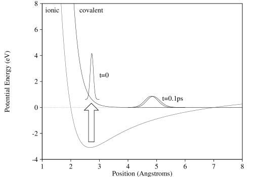
FIG. 1.: Relevant potentials for the NaI molecule with superimposed wave packets. Expressions for the ionic and covalent potentials are given in Eqs. (82) and (80). The wave packets shown for $t=0$ and $t=0.1$ ps have been scaled. The wave packet at $t=0$ has been promoted from the ionic potential to the covalent potential by an ultra-short pulse. The two wave packets shown at $t=0.1$ ps arise from the Gaussian wave packet approximation (left) and the extended Gaussian wave packet approach (right). These two wave packets are shown more clearly in Fig. 2.

FIG. 2.: Wave packet evolution in NaI after a time of 0.1 ps. The wave packet on the left (GWP) is from the Gaussian wave packet approximation, Eq. (20). The wave packet on the right (XGWP) is the extended Gaussian wave packet from Eqs. (14), (15), (25), and Eqs. (57) with six basis states.

FIG. 3.: Morse potential showing the initial Gaussian wave packet (left) and the final time evolved wave packet (right) which is shown in more detail in Fig. 4. The initial and final wave packets are shown together here to show the dramatic change of width; a situation where the extended Gaussian wave packet approach may be appropriate. The initial wave packet is located at $x=19.5$ (with a width of $1/\sqrt{2}$ in scaled units) and the final wave packet is shown for $t=70.0$ in scaled units (i.e. $m=1,\hbar=1$). The Morse potential, Eq. (89), has parameters $D=10,\beta_{M}=0.02$, and $x_{M}=60$.

FIG. 4.: Final wave packet, determined with 20 basis states (XGWP), for the evolution on the Morse potential in Fig. 3. The Gaussian wave packet (GWP) appears skewed to the left. The time elapsed since the initial state is 70.0 in scaled units.

FIG. 5.: Final wave packets, determined at $t=70$, for an initial $n=1$ wave packet located at $x=19.5$ in the potential shown in Fig. 3. The solid curve (XGWP) shows the extended Gaussian wave packet calculated in a basis of 20 states. The dashed curve (UNC) shows the final wave packet when there is no coupling between the basis states, and the initial wave packet only changes its location, width, and momentum.

REFERENCES

- [1] A.H. Zewail, Science 242, 1645 (1988); M. Gruebele and A.H. Zewail, Physics Today 43 (5), 24 (1990); A.H. Zewail, Sci. Am. 263 (12), 40 (1990); A.H. Zewail (ed.), The Chemical Bond (Academic Press, San Diego, 1992); A.H. Zewail, J. Phys. Chem. 97, 12427 (1993).
- [2] B.M. Garraway and K.-A. Suominen, Rep. Prog. Phys. 58, 365 (1995).
- [3] I.S. Averbukh and N.F. Perelman, Sov. Phys. JETP 69, 464 (1989); Phys. Lett. A 139, 449 (1989); M.J.J. Vrakking, D.M. Villeneuve, and A. Stolow, Phys. Rev. Lett. 54, 37 (1996).
- [4] C.S. Adams, M. Sigel, and J. Mlynek, Phys. Rep. 240, 143 (1994).
- [5] M. Nauenberg, C. Stroud, and J. Yeazell, Scientific American, 270, 44 (1994); M. Nauenberg, Phys. Rev. A 40, 1133 (1989); G. Alber and P. Zoller, Phys. Rep. 199, 231 (1991).
- [6] See, for example, A. Goldberg, H.M. Schey, and J.L. Schwartz, Am. J. Phys. 35, 177 (1967); J.A. Fleck, J.R. Morris, and M.D. Feit, Appl. Phys. 10, 129 (1976); M.D. Feit, J.A. Fleck, and A. Steiger, J. Comput. Phys. 47, 412 (1982); C. Leforestier, R.H. Bisseling, C. Cerjan, M.D. Feit, R. Friesner, A. Guldberg, A. Hammerich, G. Jolicard, W. Karrlein, H.-D. Meyer, N. Lipkin, O. Roncero, and R. Kosloff, J. Comput. Phys. 94, 59 (1991).
- [7] E. J. Heller, J. Chem. Phys. 62, 1544 (1975).
- [8] D. Huber and E. J. Heller, J. Chem. Phys. 87, 5302 (1987).
- [9] D. Huber and E. J. Heller, J. Chem. Phys. 89, 4752 (1988).
- [10] S.-Y. Lee and E. J. Heller, J. Chem. Phys. 76, 3035 (1982).
- [11] R.D. Coalson and M. Karplus, Chem. Phys. Lett. 90, 301 (1982).
- [12] S.-Y. Lee, Chem. Phys. 108, 451 (1986).
- [13] K.G. Kay, J. Chem. Phys. 91, 170 (1989); Phys. Rev. A 46, 1213 (1992).
- [14] J. Kucar and H.-D. Meyer, J. Chem. Phys. 90, 5566 (1989).
- [15] K.B. Møller and N.E. Henriksen, J. Chem. Phys. 105, 5037 (1996).
- [16] G.D. Billing, J. Chem. Phys. 107, 4286 (1997).
- [17] G.D. Billing, J. Chem. Phys. 110, 5526 (1999).
- [18] S. Adhikari and G.D. Billing, J. Chem. Phys. 111, 48 (1999).
- [19] R. Schack, T. A. Brun, and I. C. Percival, J. Phys. A 28, 5401 (1995); Phys. Rev. A 53, 2694 (1996).
- [20] G. Schrade, V. I. Man’ko, W. P. Schleich, and R. J. Glauber, Quantum Semiclasss. Opt. 7, 307 (1995).
- [21] C.M. Caves, Phys. Rev. D 23, 1693 (1981); D. Stoler, ibid. 1, 3217 (1970); for an overview of squeezing in the context of light see R. Loudon and P.L. Knight, J. Mod. Opt. 34, 709 (1987).
- [22] A. Mufti, H.A. Schmitt, and M. Sargent III, Am. J. Phys. 61, 729 (1993); D.R. Truax, Phys. Rev. D 31, 1988 (1985).
- [23] K.B. Møller, T.G. Jørgensen, and J.P. Dahl, Phys. Rev. A 54, 5378 (1996).
- [24] R.J. Cook and R.K. Hill, Opt. Commun. 43, 258 (1982).
- [25] G.I. Opat, S.J. Wark and A. Cimmino, Appl. Phys. B54, 396 (1992); T.M. Roach, H. Abele, M.G. Boshier, H.L. Grossman, K.P. Zetie, and E.A. Hinds, Phys. Rev. Lett. 75, 629 (1995); I.G. Hughes, P.A. Barton, T.M. Roach, M.G. Boshier, and E.A. Hinds, J. Phys. B 30, 647 (1997); I.G. Hughes, P.A. Barton, T.M. Roach and E.A. Hinds, ibid. 2119 (1997).
- [26] T.S. Rose, M.J. Rosker, and A.H. Zewail, J. Chem. Phys. 88, 6672 (1988); M.J. Rosker, T.S. Rose, and A.H. Zewail, Chem. Phys. Lett. 146, 175 (1988); V. Engel, H. Metiu, R. Almeida, R.A. Marcus, and A.H. Zewail, ibid. 152, 1 (1988); S.-Y. Lee, W.T. Pollard, and R.A. Mathies, J. Chem. Phys. 90, 6146 (1989); T.S. Rose, M.J. Rosker, and A.H. Zewail, ibid. 91, 7415 (1989); A. Mokhtari, P. Cong, J.L. Herek, and A.H. Zewail, Nature 348, 225 (1990); P. Cong, A. Mokhtari, and A.H. Zewail, Chem. Phys. Lett. 172, 109 (1990); S. Chapman and M.S. Child, J. Phys. Chem. 95, 578 (1991); H. Kono and Y. Fujimura, Chem. Phys. Lett. 184, 497 (1991); J.L. Herek, A. Materny, and A.H. Zewail, ibid. 228, 15 (1994).
- [27] S.E. Choi and J.C. Light, J. Chem. Phys. 90, 2593 (1989).
- [28] V. Engel and H. Metiu, J. Chem. Phys. 90, 6116 (1989).
- [29] M.B. Faist and R.D. Levine, J. Chem. Phys. 64, 2953 (1976).
- [30] N.J.A. van Veen, M.S. de Vries, J.D. Sokol, T.Baller, and A.E. de Vries, Chem. Phys. 56, 81 (1981).