Motion of Three Vortices near Collapse

Abstract

A system of three point vortices in an unbounded plane has a special family of self-similarly contracting or expanding solutions: during the motion, vortex triangle remains similar to the original one, while its area decreases (grows) at a constant rate. A contracting configuration brings three vortices to a single point in a finite time; this phenomenon known as vortex collapse is of principal importance for many-vortex systems. Dynamics of close-to-collapse vortex configurations depends on the way the collapse conditions are violated. Using an effective potential representation, a detailed quantitative analysis of all the different types of near-collapse dynamics is performed when two of the vortices are identical. We discuss time and length scales, emerging in the problem, and their behavior as the initial vortex triangle is approaching to an exact collapse configuration. Different types of critical behaviors, such as logarithmic or power-law divergences are exhibited, which emphasizes the importance of the way the collapse is approached. Period asymptotics for all singular cases are presented as functions of the initial vortices configurations. Special features of passive particle mixing by a near-collapse flows are illustrated numerically.

¹Courant Institute of Mathematical Sciences, New York University, 251 Mercer St., New York, NY 10012, USA

²Department of Physics, New York University, 2-4 Washington Place, New York, NY 10003, USA

1 Introduction

The importance of point vortices in applications is due to the dominant role of coherent vortical structures in many $2D$ turbulent flows. Experimental and numerical studies performed in [1]-[8] have demonstrated, that in cases of driven or freely decaying $2D$ turbulence a number of concentrated vortices develops out of an originally unstructured flow. In many situations, dynamics of this finite-size vortices can be reasonably well approximated by point-vortex models [9]-[11], allowing the reduction of the study of a time dependent field, to a simpler Hamiltonian system of $N$ interacting particles. Point-vortex dynamics is an essential ingredient of punctuated Hamiltonian models, which have been successfully used to describe the evolution of $2D$ turbulence after the emergence of the vortices [8, 12, 13]. In these models, the advection of well-separated vortices is approximated via Hamiltonian point-vortex dynamics; to account for the change in the vortex population toward smaller number of bigger vortices, dissipative merging processes [14, 15] are included for vortices which have approached each other closer than a certain critical distance. Point-vortex dynamics is responsible for bringing vortices together, i.e. it determines what kind of merger processes will occur and how often.

The number of vortices in a flow can be quite large, in which case a complete dynamical description gets intractable, but still can yield some important statistical quantities [16, 17]. On the other hand, few-vortex systems can be investigated in much more detail. Recent interest in this area was mainly directed towards the study of Lagrangian chaos in different settings [18]-[23]. Apart from this, low-dimensional vortex dynamics is essential for the understanding of the evolution of many-vortex flows, since it describes their "elementary interactions" [24]. On an unbounded plane one needs at least three vortices to get a non-trivial dynamics, leading to non-constant inter-vortex distances. On the other hand, motion of three vortices on an unbounded plane is always integrable, whereas a generic four-vortex system is already chaotic [25, 26, 27]. Hence, a three-vortex system is the only generic nontrivial case, which allows a complete dynamical analysis. General classification of different types of three vortex motion, as well as studies of special cases of particular interest were repeatedly addressed by many authors [30, 37, 24, 26, 31, 29, 32, 18], see [35] for a review.

If we think about point vortices as an approximation of a finite-size patches of concentrated vorticity, than we have to be sure that they always stay separated by a distance several times larger than a characteristic size of the patch, in order for the approximation to be valid (see [10] for a direct comparison of finite-size patch dynamics with its point vortex counterpart). A natural question is how close can the vortices approach each other during their motion? A rather surprising answer is that three vortices can be brought to a single point in finite time by their mutual interaction. Aref [35] points out that this result was already known to Gröbli more than a century ago. This phenomenon, known as point-vortex collapse was studied in [24, 29, 31, 32]. The dynamics of exact collapse is relatively simple due to a self-similarity of vortex motion in this case: a triangle formed by vortices (vortex triangle) rotates and shrinks, but stays similar to the initial one. Vortex triangle area decreases linearly with time, at a rate determined by vortex strengths and triangle shape [24]. A spatial reflection of a vortex triangle is equivalent to a time reversal, so that a reflection of a collapse configuration will experience an infinite self-similar expansion with the same rate of change of triangle area. The finite-time collapse of three point vortices into one (or its reverse the splitting of one vortex into three) changes the topology of the flow field, this feature itself has important consequences: this phenomenon may play an important role in topologically driven transitions where vortices are involved, and it conceptually allows the concentration (collapse) or spreading (splitting) of vorticity even for non-viscous media.

As a matter of fact, analysis of rare gas of vortex patches, performed in [28] indicates, that in the limit of low vortex density (vortex occupation less than one-two percent), strong interactions occur only between three vortices in a specific way, similar to the three point-vortex collapse. These processes may be thought of as resonance interactions in the vortex gas.

For the collapse to happen certain conditions on vortex strengths and initial positions have to be satisfied exactly, so that in a real system, probability of this event is zero: true resonances do not occur. However, actual vortices have some characteristic size, and when distance between them gets comparable with their size, vortices experience a considerable distortion, and may merge together, which means, that from a broader physical point of view, a collapse can be thought of as a process which brings vortices close enough (up to their size) to each other. For three initially well-separated vortices to collapse in the above sense, their strength and positions may satisfy "resonance conditions" only approximately. We refer to this kind of motion as near-collapse dynamics. Its importance stems from the fact, that inter-vortex distances are changed considerably (by orders of magnitude) during the motion, which brings the system to a different length-scale, where new physical mechanisms enter into play.

The main goal of this article is to describe different scenarios of the 3-vortex system in near-collapse dynamics, in other words we perform a quantitative analysis of the motion in near-collapse situations, when the resonance initial conditions are slightly distorted, and/or the vortex strengths are not precisely tuned. These results are briefly resumed in tables 1-3 included in Section 3. We restrict our attention to the case when two of the vortices are identical, for which it is possible to map the dynamics of the vortices to a motion of a particle in a one dimensional potential. Our description is tailored to obtain the dynamical characteristics of the motion, such as the intervals of vortex distance variation, period of relative motion, etc, and even in a simplified situation of two equal-strength vortices, we have found a rich pattern of vortices dynamics. Shortly, depending on the parameters of the system, the vortices can perform periodic dynamics with different singular periods as well as periodic dynamic with non-singular period. More importantly we have found that the singularity of the periods can be of the logarithmic or pole type. This information about possible time scalings of the near collapse motion should be taken into account when many-vortex systems are considered and, particularly it is significant for studying advection in 3-vortex systems. We will come to this issue in a forthcoming publication.

In Section 2 the basic equations of vortex motion, their symmetries and corresponding first integrals are specified. Effective Hamiltonian for a three-vortex system with two identical vortices is introduced in Section 3. Using this Hamiltonian, different types of near-collapse dynamics are classified and analyzed. In Section 4 we discuss various routes to collapse, i.e. the manner in which near-collapse motion types approach self-similarly contracting (expanding) solutions as initial configuration is taken closer to the exact resonance. In Section 5 we give an illustration of how the approach to collapse affects passive particle advection.

2 Dynamical equations

Point vortices are exact solutions of Euler equation (see for example [33]); which writes for the vorticity $\Omega$

$$\frac{\partial\Omega}{\partial t}+\left[\Omega,\psi\right]=0\>,$$ (1)

where $[\cdot,\cdot]$ is the usual Poisson bracket, and $\psi$ is the stream function; for two dimensional motion of incompressible fluid $\Omega=-\nabla^{2}\psi$. Equation (1) expresses the conservation of generalized vorticity along the path lines of the flow.

A point vortex system is defined by a vorticity distribution given by a superposition of Dirac functions:

$$\Omega({\textbf{R}},t)=\sum_{i=1}^{N}k_{i}\delta\left({\textbf{x}}-{\textbf{x}}_{i}(t)\right)\>,$$ (2)

where x is a vector in the plane of the flow, $k_{i}$ is the circulation of $i$-th vortex, $N$ is the total number of vortices, and ${\textbf{x}}_{i}(t)$ is the vortex position at time $t$. Using this expression for the vorticity, and solving Poisson equation, in the Euler case, one obtains a stream function of a point vortex system. By Helmholtz theorem [34], the motion of vortices is determined by the value of the velocity field at the position of the vortex. The equation of a point vortex motion is:

$$k_{i}\frac{d{\textbf{x}}_{i}}{dt}={\textbf{e}}_{z}\wedge\frac{\partial\psi}{\partial{\textbf{x}}_{i}}\>.$$ (3)

where ${\textbf{e}}_{z}$ is the unit vector perpendicular to the flow. The motion has an Hamiltonian structure with the two Cartesian coordinates as conjugated variables, and by convention we shall drop $\psi$ and use the notation $H$ instead. The Hamiltonian $H$ is given by:

$$H=\frac{1}{2\pi}\sum_{i>j}k_{i}k_{j}U(x_{ij})$$ (4)

where $x_{ij}=|{\textbf{x}}_{i}-{\textbf{x}}_{j}|$ and the interaction potential $U(x)=-\log(x)$ in case of an unbounded plane. The Hamiltonian (4) is invariant under translation and rotation, which implies both the conservation of the vortex momentum:

$${\textbf{P}}\equiv\sum^{N}_{i=1}k_{i}{\textbf{x}}_{i}(t)=const.$$ (5)

and vortex angular momentum $L{\textbf{e}}_{z}$ with:

$$L^{2}\equiv\sum_{i=1}^{N}k_{i}{\textbf{x}}_{i}^{2}(t)=const.$$ (6)

In this paper we consider a case of three vortices in an unbounded domain. We restrict our attention to the relative motion of vortices, taking inter-vortex distances $R_{i}$ as prime variables. The notation we use is illustrated in Fig. 1. The invariance of the Hamiltonian (4) under translations allows us a free choice of the coordinate origin, which we put to the center of vorticity (when it exists). Then, the other two constants of motion (energy and angular momentum) written in a frame independent form become:

$$\left\{\begin{array}[]{l}H=-\frac{1}{2\pi}\left[k_{1}k_{2}\ln R_{3}+k_{1}k_{3}\ln R_{2}+k_{3}k_{2}\ln R_{1}\right]\\ K=\left[\left(\sum_{i}k_{i}\right)L^{2}-P^{2}\right]=k_{1}k_{2}R^{2}_{3}+k_{1}k_{3}R^{2}_{2}+k_{3}k_{2}R^{2}_{1}\>.\end{array}\right.$$ (7)

The equations of motion (3) yield the following non canonical system for the dynamics of the inter-vortex distances:

$$\left\{\begin{array}[]{l}k^{-1}_{1}R_{1}\dot{R}_{1}=A/\pi(R^{-2}_{2}-R^{-2}_{3})\\ k^{-1}_{2}R_{2}\dot{R}_{2}=A/\pi(R^{-2}_{3}-R^{-2}_{1})\\ k^{-1}_{3}R_{3}\dot{R}_{3}=A/\pi(R^{-2}_{1}-R^{-2}_{2})\>,\end{array}\right.$$ (8)

where $A$ is the area of the triangle $A_{1}A_{2}A_{3}$ (see Fig. 1), and $\dot{x}$ refers to the time derivative of $x$, (See [24, 31] for details).

The physical system being defined, we shall now focus on the near collapse configuration. As mentioned earlier, for the three point vortex problem, under certain conditions, which depends both on the initial conditions, and the vortex strengths, the motion is self similar, leading either to the collapse of the three vortices in a finite time, or by time reversal, to an infinite expansion of the triangle formed by the vortices. These conditions of a collapse or an infinite expansion of the three point vortices are easily found. The first condition is immediate as for a collapse to occur $K$ has to vanish. For the second condition we just need to look for conditions to obtain a scale invariant Hamiltonian. With such spirit let us divide all lengths $R_{i}$ by a common factor $\lambda$ in the Hamiltonian $H$. We readily obtain $H^{\prime}(\lambda)=H+\left(\sum k_{i}k_{j}\right)\ln\lambda$, we then obtain the collapse conditions:

$$K=0$$ (9)

$$\sum_{i}\frac{1}{k_{i}}=0\>,$$ (10)

i.e, the harmonic mean of the vortex strengths (10) and the total angular momentum in its frame free form (9), are both zero. Near a collapse configuration, the two conditions (9), (10) allow two different ways to approach the singularity. Namely, we can change initial conditions which changes the value of $K$, or change the vortex strength and modify the harmonic mean. Unfortunately the motion of the three vortices even though integrable is not easily computed analytically. It then seemed useful to restrict the problem to some less general case, assuming that the basic mechanisms of collapse should not differ much in the general case. To emphasize this last statement, let us first consider a general collapse situation, for which the total strength is $k_{tot}$. The following conditions are then fulfilled

$$\sum_{i}k_{i}=k_{tot}\>,\sum_{i}\frac{1}{k_{i}}=0\>,$$ (11)

which are equivalent to

$$\sum_{i}k_{i}=k_{tot}\>,\sum_{i}k^{2}_{i}={k_{tot}}^{2}\>.$$ (12)

The values for the vortex strengths corresponding to a collapse configuration are therefore located on the circle resulting from the intersection of the sphere of radius ${k_{tot}}^{2}$ and the plane imposing a total vortex strength equal to $k_{tot}$. Since we have a circle, we shall assume that, from this point of view, no special configuration exists, and any should be sufficient to describe qualitatively the different possible behaviors.

In the following we will be considering the case, when two of the three vortices are identical. Since the rescaling of time scales leads to a freedom in vortex strength normalization, we will assume

$$k_{2}=k_{3}=1$$ (13)

Then, in order for a collapse to happen, the strength of the third vortex has to satisfy (10) which gives the resonance value of the first vortex: $k_{1c}=-1/2$. We will be mostly interested in the situations, when $k_{1}$ is negative and close to its resonance value, so we will denote

$$k\equiv|k_{1}|\>,$$ (14)

and define the deviation from the resonance as

$$\delta=1/2-k\>.$$ (15)

3 Near-collapse dynamics of vortices

In the case when two out of three vortices are identical, there exists a convenient representation of the system dynamics in terms of a motion of a particle in a one-dimensional potential, parametrically depending on vortex initial condition. To derive this representation, we introduce a new set of variables: $X=R^{2}_{1}$, $Y=R^{2}_{2}R^{2}_{3}$, and $Z=R^{2}_{2}+R^{2}_{3}$. The constants of motion (7) can be written as:

$$\left\{\begin{array}[]{l}\Lambda=e^{4\pi H}=Y^{k}/X\\ K=X-kZ\>.\end{array}\right.$$ (16)

where new parameter $\Lambda$ is introduced instead of $H$ in order to simplify formulas.

An equation on $X$ can be directly obtained from the first equation of (8), squaring it gives:

$$\dot{X}^{2}=\frac{4}{\pi^{2}}A^{2}k^{2}\frac{(R_{2}^{2}+R^{2}_{3})^{2}-4R^{2}_{2}R^{2}_{3}}{R_{2}^{4}R^{4}_{3}}=\frac{4}{\pi^{2}}A^{2}k^{2}\frac{Z^{2}-4Y}{Y^{2}}\>.$$ (17)

Square of the vortex triangle area $A$ can be found from geometrical identities

$$\left\{\begin{array}[]{l}A=\sqrt{Y}|\sin\theta|/2\\ X=Z-2\sqrt{Y}\cos\theta\>,\end{array}\right.$$ (18)

which leads to

$$16A^{2}=4Y-(X-Z)^{2}\>.$$ (19)

Using the expression for the constants of motion (16), we obtain:

$$\dot{X}^{2}=\frac{1}{4\pi^{2}}\frac{[4k^{2}Y-(K-(1-k)X)^{2}][(K-X)^{2}-4k^{2}Y]}{k^{2}Y^{2}},$$ (20)

where $Y=(\Lambda X)^{1/k}$. This equation has a form of an energy conservation law for a particle of mass $1$ and zero total energy moving in a potential $V(X;\Lambda,K,k)$, defined by

$$V(X;\Lambda,K,k)\equiv\frac{{[(K-(1-k)X)^{2}-4k^{2}Y][(X-K)^{2}-4k^{2}Y]\}}}{8\pi^{2}k^{2}Y^{2}}\>.$$ (21)

Indeed, equation (20) can be rewritten as

$$H_{eff}(\dot{X},X;\Lambda,K,k)\equiv P^{2}/2+V(X;\Lambda\,K,k)=0\>,$$ (22)

with Hamiltonian equations

$$\dot{X}=\partial H_{eff}/\partial P\equiv P\>,\hskip 28.45274pt\dot{P}=-\partial H_{eff}/\partial X\>.$$ (23)

Thus, dynamics of vortex configuration is governed by an effective Hamiltonian $H_{eff}$, where the shape of the potential well $V$ depends on the initial vortex positions through the values of first integrals $\Lambda$ and $K$ (16), and the strength of the first vortex $k$.

Effective Hamiltonian representation (22), gives a number of advantages, allowing to use simple standard techniques for one-dimensional conservative systems to find dynamical properties of vortex motion. In a sense, the problem is reduced to determining the shape of the potential $V$ as a function of its parameters.

Before proceeding to the analysis of the types of potentials, emerging in our problem, we have to mention the restrictions, imposed on the system by the fact that three vortices form a triangle. Since this was not taken into account in the derivation of the effective Hamiltonian (22), it may put additional boundaries on the possible values of $X$. Note, that since the effective energy $H_{eff}$ in (22) is always zero, a motion exists only on the segments where the potential is negative. Therefore, triangle inequalities and the condition $V\leq 0$ define the physical domain of $X$. Triangle inequalities

$$|R_{2}-R_{3}|\leq R_{1}\leq R_{2}+R_{3}\>,$$ (24)

written in terms of new variables can be obtained by taking the square of (24): $Z-2\sqrt{Y}\leq X\leq Z+2\sqrt{Y}$, which is equivalent to

$$(X(k-1)+K)^{2}-4k^{2}Y\leq 0\>.$$ (25)

The condition (25) is equivalent to the positiveness of the right hand side of equation (19) and translates that the square of the area of the triangle $A_{1}A_{2}A_{3}$ is positive. The condition $V(X)\leq 0$ together with the triangle inequalities (25) imposes then

$$(K-X)^{2}-4k^{2}Y\geq 0\>,$$ (26)

Recalling that $Z>0$, we have $X\geq K$, which together with inequality (26), gives finally

$$X\geq K+2k\sqrt{Y}\>.$$ (27)

Now we have a precise information on where the motion should lie, and can proceed to the study of different regimes of near-collapse dynamics. Although the effective potential representation is valid for any $k\neq 0$, we will restrict our study (and our definition of “near-collapse”) to the interval $k\in]0;1[$, since the special cases $k=1$ (escaping vortex pair) and $k=2$ (neutral tripole), as well as the degenerate case $k=0$ (two vortices and a passive particle) bring up their specific singularities, unrelated to the collapse phenomenon. Let us consider different regimes such that each regime corresponds to a class of qualitatively similar motions [24]. Using the effective Hamiltonian representation (22), we infer that different regimes may be encountered corresponding to the number of roots of the potential $V(X;\Lambda,K,k)$ lying within the physical domain. This number changes with variation of the parameters $(\Lambda,K,k)$.

Note, that the absolute value of $K$ depends on the length units and can be scaled out of the problem. Indeed, the potential $V$ and the physical domain boundary (27) are invariant under the scaling transformation (compare to (16))

$$X\rightarrow\frac{X}{|K|},\hskip 28.45274pt\Lambda\rightarrow\Lambda|K|^{\delta}\>,$$ (28)

and the problem can be reduced to the study of the three following cases

$$K=1\>,\;K=-1\>,\;K=0\;,$$ (29)

where the last case is singular. The different situations encountered have been condensed in the tables 1-3, which are presented at the end of this Section. This is intended to briefly summarize the result of this work and allow the reader to browse through this paper more easily.

In the following we will discuss in details the different types of motions and critical situation encountered; most of the figures illustrating the problem will correspond to the values (29), although we will keep $K$ as a scale parameter in formulas, keeping in mind, that only its sign is relevant to distinguish different regimes. We insist that the scaling of $\Lambda$ in (28), which can be rewritten in terms of vortex energy (7) as

$$H\rightarrow H+\delta\ln|K|\>,$$ (30)

leaves $\Lambda$ and $H$ unchanged, when $\delta=0$, i.e. when vortex strengths exactly satisfy the collapse condition (10). The scales of the motion are determined by the value of the angular momentum $K$, while from a pure energetic point of view the motion would be thought as scale invariant.

3.1 Critical situations for $K\neq 0$

To detect bifurcations, leading to the appearance of new roots of the potential, we look for the degenerate roots of (21). As a first step, we just want to find these roots, leaving their detailed interpretation for the following paragraphs. Such roots $X_{c}$ exist only for certain critical values $\Lambda_{c}$ of the energy parameter $\Lambda$, and can be found from:

$$\left\{\begin{array}[]{l}V(X_{c},\Lambda_{c})=0\\ \partial V/\partial X(X_{c},\Lambda_{c})=0\end{array}\right.$$ (31)

The above system can be easily solved if one notices, that the potential (21) is written in a factorized form: $V=V_{1}*V_{2}/(8\pi^{2}k^{2}Y^{2})$, with

$$V_{1}\equiv[(K-(1-k)X)^{2}-4k^{2}Y],\hskip 28.45274ptV_{2}\equiv[(K-X)^{2}-4k^{2}Y]$$ (32)

Then, if a solution $X_{c},\,\,\Lambda_{c}$ exists and is different from $X=0$, it should be either a double zero of $V_{1}$ or $V_{2}$, or a zero of both $V_{1}$ and $V_{2}$.

We start from finding a double zero of $V_{2}$, which yields a system similar to (31), where $V$ is substituted by $V_{2}$, that leads to:

$$\left\{\begin{array}[]{l}\left(X-K\right)^{2}-4k^{2}Y=0\\ 2kX\left(X-K\right)-4k^{2}Y=0\end{array}\right.$$ (33)

and after some substitutions we readily obtain,

$$\left\{\begin{array}[]{l}X_{c_{1}}=K/2\delta\\ \Lambda_{c_{1}}=\left(K/2\delta\right)^{-2\delta}\end{array}\right.$$ (34)

For $X_{c_{1}}$ to be positive, $K$ and $\delta$ must have the same sign, so this bifurcation pertains to the physical region only for the cases $K>0,\,\,k<1/2$ and $K<0,\,\,k>1/2$ (it is easy to check that substitution of (34) into (27) turns the latter into an identity). Another solution, $X=K,\,\,\Lambda=0$, corresponds to the situation when the negative vortex merges with one of the two others, reducing the system to a two-vortex case. Notice that $X_{c_{1}}$ diverge as vortex strength collapse condition (10) is approached ($\delta\rightarrow 0,k\rightarrow 1/2$), which announces a special behavior of the case $\delta=0$, requiring a special treatment.

Double zeros of $V_{1}$ are found in the same manner. After some algebra we obtain:

$$\left\{\begin{array}[]{l}X_{c_{2}}=X_{c_{1}}/\left(1-k\right)\\ \Lambda_{c_{2}}=(1+2\delta)\Lambda_{c_{1}}/2\end{array}\right.$$ (35)

and a solution $X=K/(1-k),\,\,\Lambda=0$ for the merged situation. Being proportional to $X_{c_{1}}$, $X_{c_{2}}$ diverges in the same manner as $\delta\rightarrow 0$, and requires sign of $K$ and $\delta$ to be the same, in order to lie in a physical range. It also diverges when $k\rightarrow 1$, as we have mentioned earlier, this is the case of a scattering of a neutral vortex pair on a vortex, which is out of the scope of the present paper. Finally we note, that since $V_{1}$ is proportional to the area of the vortex triangle $A$, the critical equilibrium position $X_{c_{2}}$ corresponds to an aligned vortex configuration; in a similar manner we deduce that $X_{c_{1}}$ corresponds to an equilateral configuration [24, 31].

A third possibility, when both $V_{1}=0$ and $V_{2}=0$, leads to the following system:

$$\left\{\begin{array}[]{l}\left(X-K\right)^{2}-4k^{2}Y=0\\ (K-(1-k)X)^{2}-4k^{2}Y=0\end{array}\right.$$ (36)

which yields:

$$\left\{\begin{array}[]{l}X_{c_{3}}=2K/(2-k)\\ \Lambda_{c_{3}}=\left[K/\left(3+2\delta\right)\right]^{-2\delta}/4\;.\end{array}\right.$$ (37)

This critical case also corresponds to an aligned configuration, where the negative vortex of strength $-k$ is in the middle between the two identical vortices. In near collapse situation $2-k>0$, and since $X_{c_{3}}$ has to be positive, this critical situation appears only for positive total vortex angular momentum $K>0$. Here a merged solution also exists ($X=0,\,\,\Lambda=+\infty$), which corresponds to the merging of the two identical vortices. We also notice that the divergence of $X_{c_{3}}$ for $k=2$ corresponds to a special case of a neutral tripole, when the total vorticity is zero, and the center of vorticity is not defined.

Now we turn our attention to the three different specific cases distinguished by the sign of $K$. For each case, we will indicate which of the above found bifurcations do occur, and study the phase space trajectories of the effective Hamiltonian (22) for different regimes.

3.2 The case $K>0$, $k\neq 1/2$

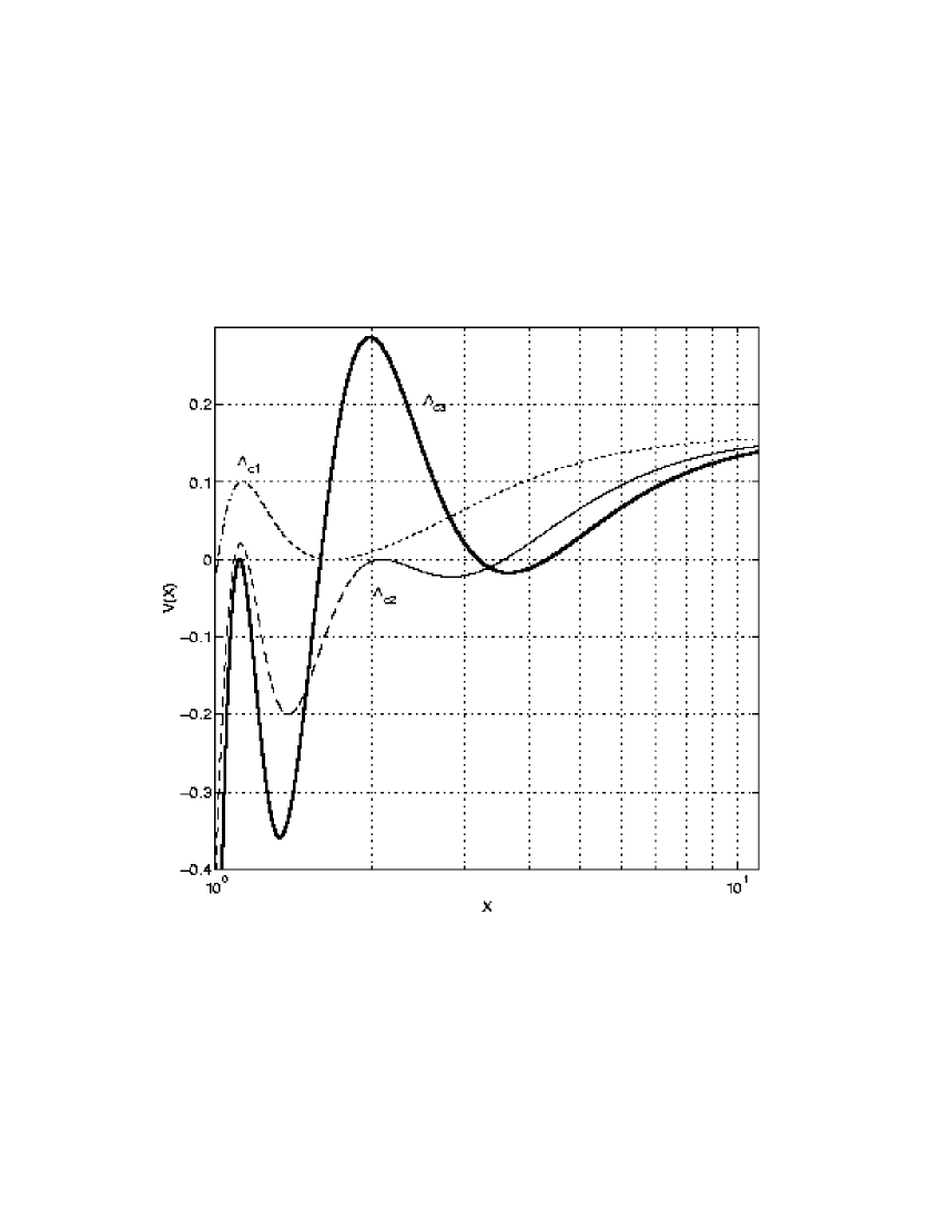
Figure 2: The potential $V(X)$ for the three critical cases. $k=0.2$. For $\Lambda=\Lambda_{c_{1}}$ the motion appears, for $\Lambda=\Lambda_{c_{2}}$ two motions are possible, and for $\Lambda=\Lambda_{c_{3}}$ an unstable aligned configuration is approached as $X\rightarrow X^{+}_{c_{3}}$.

From the previous Section, we know that the number of critical energies for this case depends on the sign of $\delta$, i.e. whether $k>1/2$ or $k<1/2$. A special case $k=1/2,\,\,\delta=0$ will be treated separately. We start from the case $k<1/2$, when all three critical cases (34), (35), (37) belong to the physical region. If we keep the value of $k$ fixed, and vary the energy, we will encounter various motion regimes, separated by the three critical energies. To illustrate the critical situations we plotted the potential $V$ as a function of $X$ for the three different critical energies for $k=0.2$ in Fig. 2. The critical energy $\Lambda_{c_{1}}$ corresponds to the maximum possible value for which motion can exist; for $\Lambda=\Lambda_{c_{2}}$ an unstable equilibrium (saddle point) appears, and motion becomes aperiodic; and in the last case of $\Lambda=\Lambda_{c_{3}}$, another saddle point appears right on the border of the physical region (corresponding to unstable aligned configuration).

Motions regimes for different energy ranges are listed below (See Table 1):

1. $\Lambda>\Lambda_{c_{1}}$ Motion impossible.

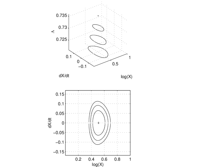
Figure 3: Phase space portrait close to $\Lambda_{c_{1}}$ for different energies for the case $K=1$ and $k=0.2$. The bottom figure is the top view of the upper one. Once the first critical situation is reached a motion is possible.

2. $\Lambda_{c_{1}}>\Lambda>\Lambda_{c_{2}}$ The potential has 2 zeros in the physical region, there exists a single type of periodic motion (see Fig. 3). When $\Lambda\rightarrow\Lambda_{c_{2}}$, the period diverges logarithmically

   $$T(\Lambda)\sim 1/2\ln|\Lambda-\Lambda_{c_{2}}|\>,$$ (38)

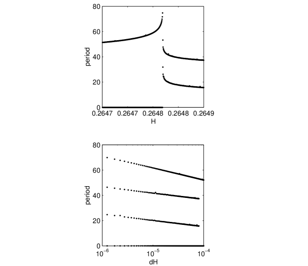
Figure 5: Period of the motion versus energy ($\Delta H=|H(X)-H_{c_{2}}|$) for $k=0.2$ close to $\Lambda=\Lambda_{c_{2}}$. We notice the logarithmic behavior of the divergence, we note also that the sum of the slopes of the two right branches (lower) is equal to the slope of the left branch (upper).

   (see Fig. 5) due to proximity of a saddle-point; motion acquires typical near-separatrix character of relatively short velocity pulses separated by long stays in the saddle-point vicinity.

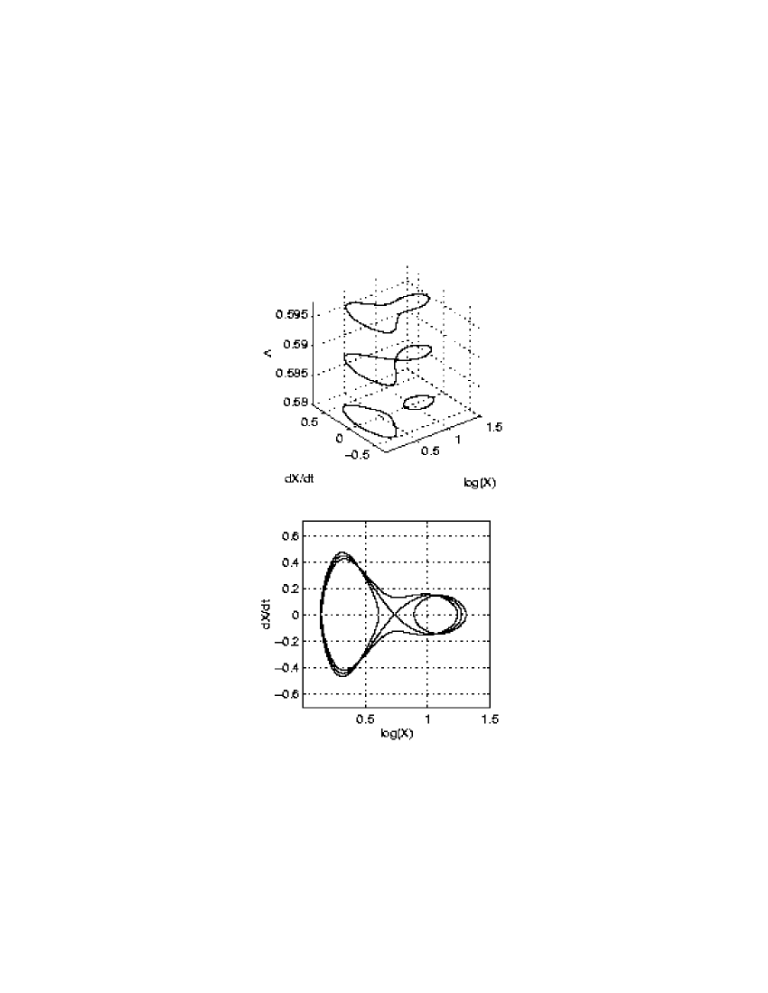
Figure 4: Phase space portrait close to $\Lambda_{c_{2}}$ for different energies for the case $K=1$ and $k=0.2$. The bottom figure is the top view of the upper one. Once the second critical situation is reached, the single possible trajectory reaches the separatrix, and the splitting in two possible motions occurs.

3. $\Lambda_{c_{2}}>\Lambda>\Lambda_{c_{3}}$ The potential has 4 zeros and two different types of periodic motion exist (see Fig. 4). Their period diverges as

   $$T(\Lambda)\sim 1/4\ln|\Lambda-\Lambda_{c_{2}}|\>,$$ (39)

   when $\Lambda$ approaches $\Lambda_{c_{2}}$, Fig. 5.

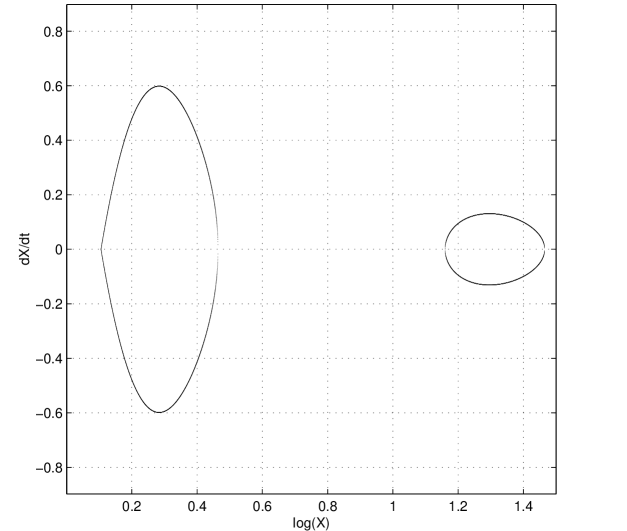
Figure 6: Phase space portrait for $\Lambda=\Lambda_{c_{3}}$ for the case $K=1$ and $k=0.2$. A splitting occurs like for $\Lambda=\Lambda_{c_{2}}$ but the triangle conditions prevent the existence of a third branch. We notice the sharp angle at $X=X_{c_{3}}$.

4. $\Lambda_{c_{3}}>\Lambda$ The potential has 4 zeros and two different types of periodic motion exist (see Fig. 6). As $\Lambda\rightarrow\Lambda_{c_{3}}$ (from both sides), the small-scale branch approaches a near-separatrix regime, its period diverges as

   $$T(\Lambda)\sim\ln|\Lambda-\Lambda_{c_{3}}|\>,$$ (40)

   for $\Lambda=\Lambda_{c_{3}}$ this branch becomes aperiodic.

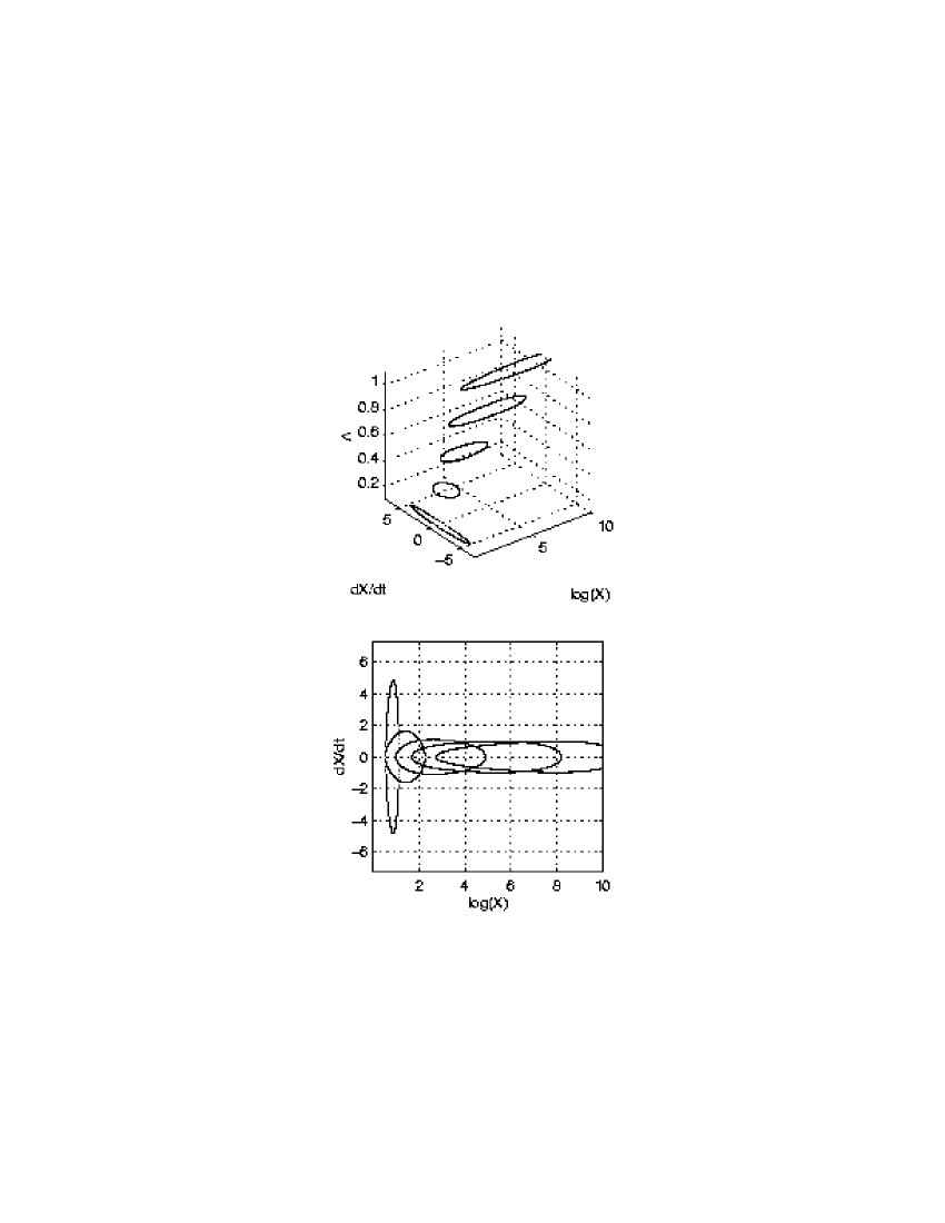
Figure 7: Phase space portrait for different values of $\Lambda$ in the case $K=1$ and $k=0.55$. The bottom figure is the top view of the upper one. The motion remains periodic. As $\Lambda$ increases, we notice the growth of the range of length scales explored by the motion.

For the case $k>1/2$ only the critical value of $X_{c_{3}}$ lies in the physical region, and only one regime of periodic motion exists (see Fig. 7).

3.3 The case $K<0$, $k\neq 1/2$

When the total vortex angular momentum is negative, the critical root (37) lies outside the physical region, and therefore we expect less variety of motion types. Otherwise, this case is similar to the $K>0$ case, in the sense that most phenomena described for $K>0$ occur, but in a reverse order; for instance, when $k>1/2$ we have three different regimes, which are analogue to the regimes of $K>0$, $k<1/2$ case. The different regimes, illustrated by their phase portraits, are listed below (See Table 1):

1. $\Lambda<\Lambda_{c_{1}}$ Motion impossible.

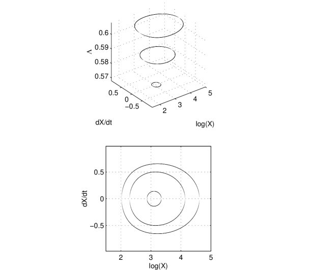
Figure 8: Phase space portrait close to $\Lambda_{c_{1}}$ for different values of $\Lambda$ in the case $K=-1$ and $k=0.55$. The bottom figure is the top view of the upper one. Once the first critical situation is reached a motion is possible.

2. $\Lambda_{c_{2}}<\Lambda<\Lambda_{c_{1}}$ The potential has 2 zeros and a periodic motion is possible (see Fig. 8). In vicinity of a saddle point ($\Lambda\approx\Lambda_{c_{2}}$) motion period diverges in the same way as in $K>0$ case.

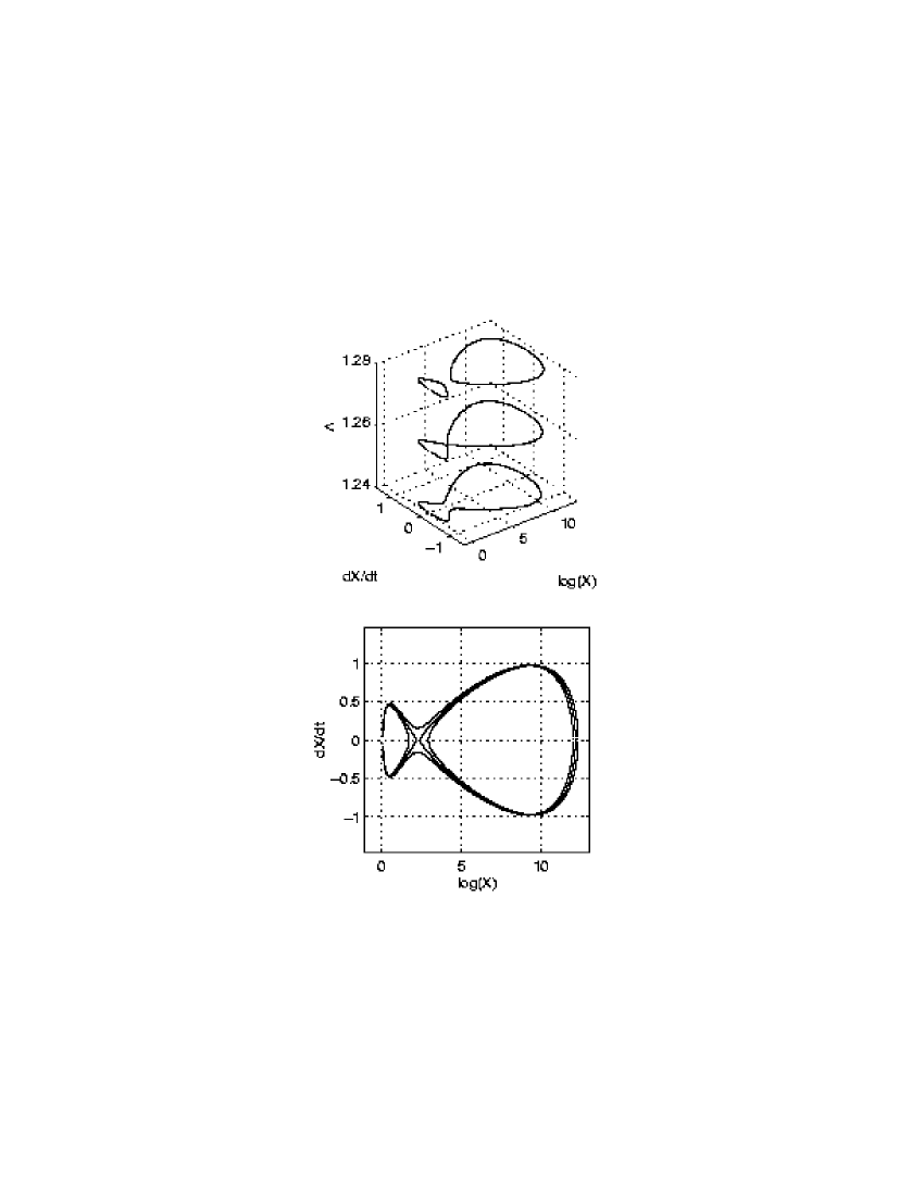
Figure 9: Phase space portrait close to $\Lambda_{c_{2}}$ for different values of $\Lambda$ in the case $K=-1$ and $k=0.55$. The bottom figure is the top view of the upper one. Once the second critical situation is reached, the single possible trajectory reaches the separatrix, and the splitting in two possible motions occurs.

3. $\Lambda_{c_{2}}<\Lambda$ The potential has 4 zeros and two different periodic motions are possible (see Fig. 9).

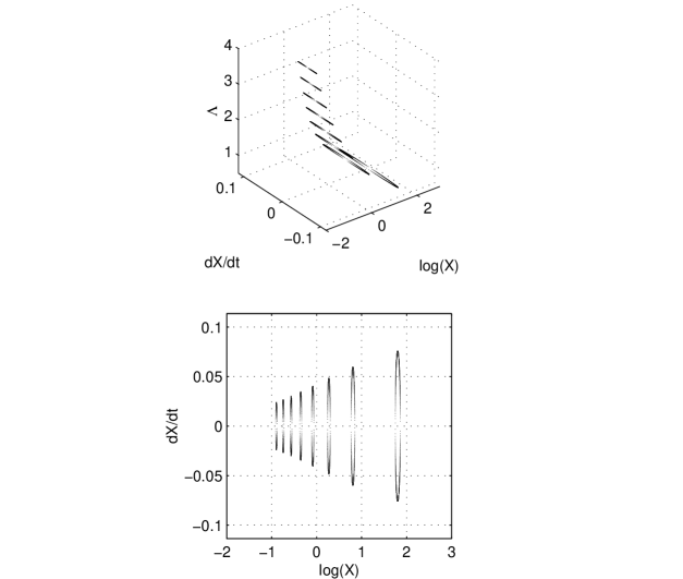
Figure 10: Phase space portrait for different values of $\Lambda$ in the case $K=-1$ and $k=0.2$. The bottom figure is the top view of the upper one. The value of $\Lambda$ determines the typical length scale of the periodic motion (the value of $K$ is fixed).

On the other hand the situation when $k<1/2$, is analogous to the $K>0$ and $k>1/2$ situation. Namely, non of the critical values are physical, and we have only one type of periodic motion for all range of energies, see Fig. 10.

Now all the possible generic situations being described, we will proceed to the important singular cases $K=0$ or $k=1/2$.

3.4 The case $K=0$.

In this situation any rescaling of length does not affect the value of $K$, and it is only the value of $\Lambda$ that controls motion scales in the system. The expression for the effective potential $V(X)$ can be considerably simplified. It is convenient to introduce new variable

$$U=\frac{X^{2}}{4k^{2}Y},$$ (41)

then (21) becomes

$$V(U)=\frac{2}{\pi^{2}}k^{2}\left(1-k\right)^{2}\left(U-\frac{1}{\left(1-k\right)^{2}}\right)\left(U-1\right)\>.$$ (42)

The zeros are simple and the different conditions imposed on $X$ imply a motion confined between

$$1\leq U\leq\frac{1}{\left(1-k\right)^{2}}\>,$$ (43)

In this situation double zero do not occur. Note that for exact collapse case, $k=1/2$, transformation to new variable (41) is singular and does not work. In this case the potential $V(X)$ is constant; its value is negative only in a range of energies $\Lambda\in[1/2,1]$, which means, that collapse configurations have their energies confined to this interval. We will return to the discussion of collapse configurations in Section 4.

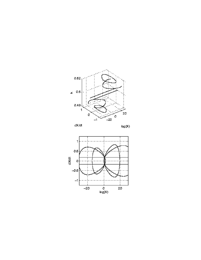
Figure 11: Phase space portrait close to $\Lambda_{c_{2}}$ for different values of $k$ in the case $K=0$. The bottom figure is the top view of the upper one.For this singular case we notice the two lines at $k=1/2$ corresponding one to collapse and one to infinite expansion. On the projection plot (bottom), the trajectories $k<1/2$ and $k>1/2$ seem to intersect on those two lines. For $\Lambda<\Lambda_{c_{2}}$ collapse is not possible, and the trajectories do not intersect. We notice that close to the collapse condition $k=1/2$, the values $k<1/2$ describe a collapse motion, while $k>1/2$ describes the expansion motion.

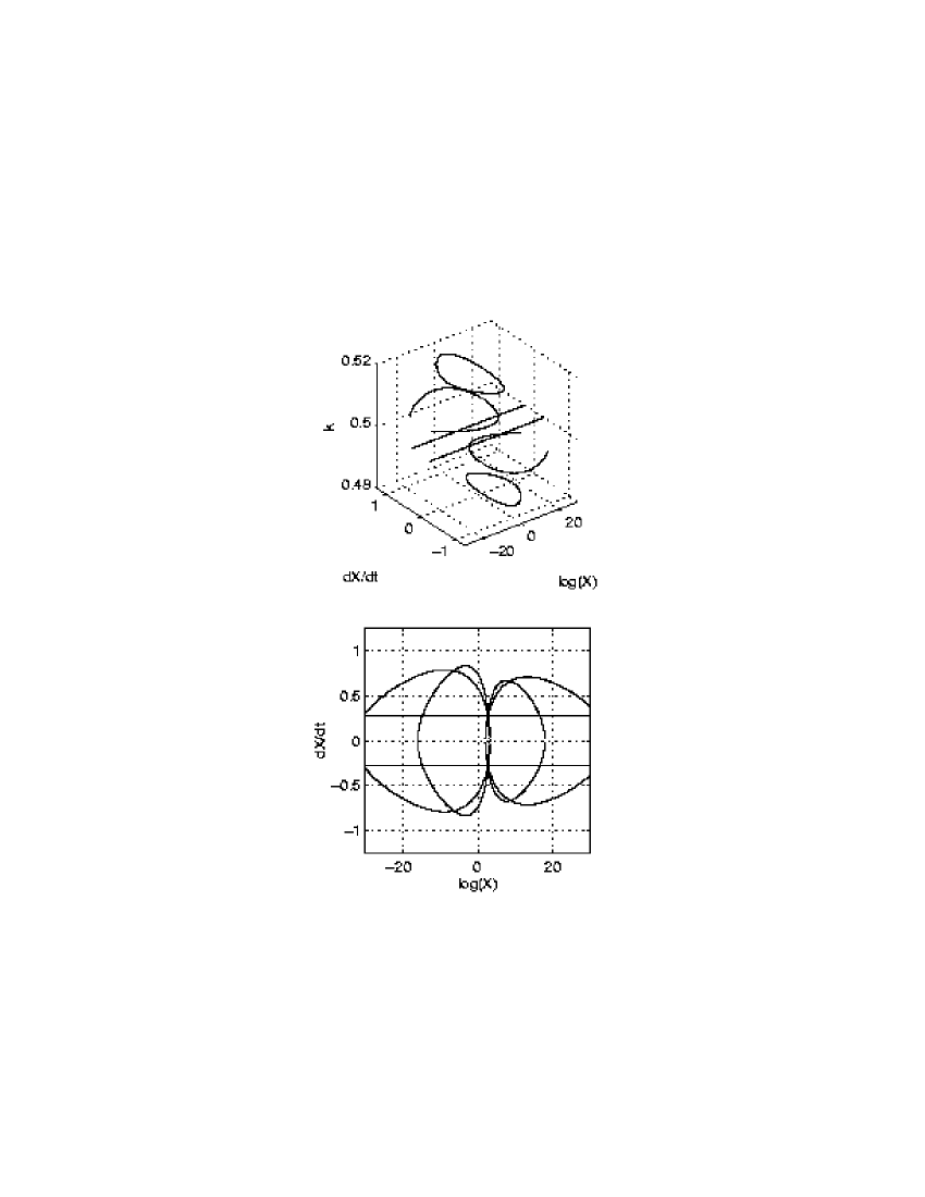
Figure 12: Phase space portrait close to $\Lambda_{c_{1}}$ for different values of $k$ for the case $K=0$. The bottom figure is the top view of the upper one.For this singular case we notice the two lines at $k=1/2$ corresponding one to collapse and one to infinite expansion. On the projection plot (bottom), the trajectories $k<1/2$ and $k>1/2$ seem to intersect on those two lines. For $\Lambda>\Lambda_{c_{1}}$ collapse is not possible, and the trajectories do not intersect. We notice that close to the collapse condition $k=1/2$, the values $k<1/2$ describe a collapse motion, while $k>1/2$ describes the expansion motion.

In this singular case, to visualize the approach to collapse ($k\rightarrow 1/2$), it is better to have $k$ fluctuating and $\Lambda$ fixed. This is due to the fact that, when $k=1/2$, which corresponds to the merging conditions, the motion is possible only within a range of energies $\Lambda_{2}>\Lambda>\Lambda_{1}$. The phase portrait of trajectories taken for different values of $k$ is shown in Fig. 11 and Fig. 12. These two figures are taken close to the values $\Lambda=1/2$ and $\Lambda=1$; we notice for the $k=1/2$ case two straight lines corresponding to the two possible motions of expansion or collapse. Note, that when $\Lambda\notin[1/2\>,\;1]$ a collapse cannot occur, which means that the trajectories for $k<1/2$ and $k>1/2$ are similar to those shown in Fig. 11, but do not intersect on the top view, the results are summarized in Table 2.

3.5 The case $k=1/2$

This special case corresponds to “scale invariance”, meaning that any length can be rescaled without changing the energy of the system. Therefore the energies of the critical situations should not depend on the value of $K$, which is scale dependent. The effective potential is now simply a fraction of polynomial and can be rewritten as

$$V(X)=\lambda\left(X-X_{1}\right)\left(X-X_{2}\right)\left(X-X_{3}\right)\left(X-X_{4}\right)/X^{4}\>,$$ (44)

where

$$X_{1}=\frac{K}{1/2-\Lambda}\>,\;X_{2}=\frac{K}{1/2+\Lambda}\>,\;X_{3}=\frac{K}{1-\Lambda}\>,\;X_{4}=\frac{K}{1+\Lambda}\>,$$ (45)

and

$$\lambda=\frac{(1/2+\Lambda)(1/2-\Lambda)(1+\Lambda)(1-\Lambda)}{4\pi^{2}\Lambda^{2}}\>.$$ (46)

We have three critical values, the first two $\Lambda_{c_{1}}=1$ and $\Lambda_{c_{2}}=1/2$ correspond to the divergence of one root, while the third $\Lambda_{c_{3}}=1/4$ corresponds to a double root situation $X_{2}=X_{3}$. Depending on the sign of $K$ we have the following allowed supports (See Table 3):

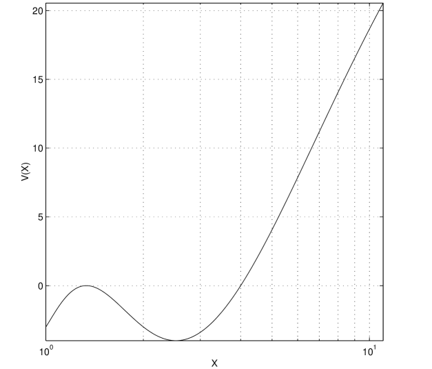
Figure 13: The effective potential $V(X)$ in the singular case $k=1/2$ ($\delta=0$) for the critical energy corresponding to $\Lambda=1/4$: the double root case.

1. $K>0$ and $\Lambda<\Lambda_{c_{3}}$ implies $X_{1}>X>X_{2}$. The potential $V(X)$ for the critical situation $\Lambda=1/4$ is illustrated on Fig. 13. As we approach collapse ($K\rightarrow 0$) this motion vanishes.

2. $K>0$ and $\Lambda_{c_{3}}<\Lambda<\Lambda_{c_{2}}$ implies $X_{1}>X>X_{3}$. The potential $V(X)$ for the critical situation $\Lambda=1/2$ is illustrated on Fig. 14. As we approach collapse ($K\rightarrow 0$) this motion also vanishes. Nevertheless this case is interesting as an aperiodic motion very close to collapse is reached as $\Lambda\rightarrow 1/2$. The period of the motion as a function of $|\Lambda-1/2|$ is shown in Fig. 15. It diverges according to a power law:

   $$T\sim\left(\Lambda-1/2\right)^{-3/2}\>,$$ (47)

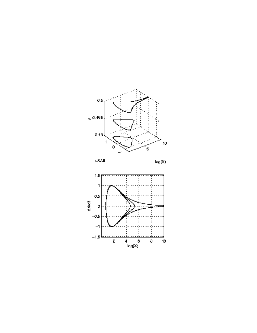
Figure 16: Phase space portrait for different values of $\Lambda$ close to $\Lambda_{c}=1/2$, in the case $K=1$ and $k=1/2$ ($\delta=0$). The bottom figure is the top view of the upper one. We notice the singular evolution of the motion to larger scales as $\Lambda$ approaches $\Lambda_{c}$.

   (see the Appendix for its derivation). Phase space portraits of the trajectories are illustrated in Fig. 16.

3. $K>0$ and $\Lambda_{c_{2}}<\Lambda<\Lambda_{c_{1}}$, then $X>X_{3}$. This motion is the closest to the collapse, as infinite expansion is possible, but $X$ is bounded from below. In this situation we may see a collapse course, which rebounds on $X_{3}$ and goes for an infinite expansion. As we approach collapse ($K\rightarrow 0$) $X_{3}\rightarrow 0$, and depending on the sign of $\dot{X}$ a full collapse can occur.

4. $K>0$, $\Lambda_{c_{1}}<\Lambda$ and $K<0$, $\Lambda<\Lambda_{c_{2}}$ motion impossible.

5. $K<0$ and $\Lambda_{c_{2}}<\Lambda<\Lambda_{c_{1}}$ , then $X>X_{1}$. We have a similar situation as the one discussed for the $K>0$ and $\Lambda_{c_{2}}<\Lambda<\Lambda_{c_{1}}$.

6. $K<0$ and $\Lambda_{c_{1}}<\Lambda$, then $X_{3}>X>X_{1}$. Here we can anticipate a similar situation as the one discussed for the $K>0$ and $\Lambda_{c_{3}}<\Lambda<\Lambda_{c_{2}}$.

In this section all possible types of motion have been discussed, all the results for the different cases are summarized in the Tables 1-3. A more detailed discussion of the vortices behavior and trajectories, as the collapse configuration is approached, is presented in the next Section.

$\Lambda$	Type of motion	Period	$K$	$k$
$\Lambda>\Lambda_{c_{1}}$	no motion	no period	$K>0$	$k<1/2$
$\Lambda_{c_{1}}>\Lambda>\Lambda_{c_{2}}$	periodic motion	$T\approx 1/2\ln|\Lambda-\Lambda_{c_{2}}|$	$K>0$	$k<1/2$
$\Lambda_{c_{2}}>\Lambda>\Lambda_{c_{3}}$	2 different periodic motions,	$T\approx 1/4\ln|\Lambda-\Lambda_{c_{2}}|$	$K>0$	$k<1/2$
	1 large scale, 1 small scale
$\Lambda_{c_{3}}>\Lambda$	2 different periodic motions,	$T\approx\ln|\Lambda-\Lambda_{c_{3}}|$	$K>0$	$k<1/2$
	1 large scale, 1 small scale
any $\Lambda$	periodic motion	no singularities for $T$	$K>0$	$k>1/2$
$\Lambda<\Lambda_{c_{1}}$	no motion	no period	$K<0$	$k>1/2$
$\Lambda_{c_{1}}<\Lambda<\Lambda_{c_{2}}$	periodic motion	$T\approx 1/2\ln|\Lambda-\Lambda_{c_{2}}|$	$K<0$	$k>1/2$
$\Lambda_{c_{2}}<\Lambda$	2 different periodic motions,	$T\approx 1/4\ln|\Lambda-\Lambda_{c_{2}}|$	$K<0$	$k>1/2$
	1 large scale, 1 small scale
any $\Lambda$	1 periodic motion	no singularities for $T$	$K<0$	$k<1/2$

Table 1: Different types of motion for the general situation $K\neq 0\>,k\neq 1/2$. The different critical values are

$\Lambda_{c_{1}}=(2\delta/K)^{2\delta}$, $\Lambda_{c_{2}}=\frac{1}{2}(1+2\delta)(2\delta/K)^{2\delta}$, $\Lambda_{c_{3}}=\frac{1}{4}[(3+2\delta)/K]^{2\delta}$.

$\Lambda$	Type of motion	Period	$K$	$k$
any $\Lambda$	periodic motion, small scales	period found numerically	$K=0$	$k<1/2$
$1/2<\Lambda<1$	collapse or expansion	aperiodic motion	$K=0$	$k=1/2$
any $\Lambda$	periodic motion, large scales	period found numerically	$K=0$	$k>1/2$

Table 2: Different types of motion for the special situation $K=0\>,k\neq 1/2$.

$\Lambda$	Type of motion	Period	$K$	$k$
$\Lambda<\Lambda_{c_{3}}$	periodic motion	$T\approx\ln|\Lambda-\Lambda_{c_{3}}|$	$K>0$	$k=1/2$
$\Lambda_{c_{3}}<\Lambda<\Lambda_{c_{2}}$	periodic motion	$T\approx|\Lambda-\Lambda_{c_{2}}|^{-3/2}$	$K>0$	$k=1/2$
$\Lambda_{c_{2}}<\Lambda<\Lambda_{c_{1}}$	aperiodic motion	no period ∗	$K>0$	$k=1/2$
$\Lambda_{c_{1}}<\Lambda$	no motion	no period	$K>0$	$k=1/2$
$\Lambda<\Lambda_{c_{2}}$	no motion	no period	$K<0$	$k=1/2$
$\Lambda_{c_{2}}<\Lambda<\Lambda_{c_{1}}$	aperiodic motion	no period ∗∗	$K<0$	$k=1/2$
$\Lambda_{c_{1}}<\Lambda$	periodic motion	$T\approx|\Lambda-\Lambda_{c_{1}}|^{-3/2}$	$K<0$	$k=1/2$

Table 3: Different types of motion for the special situation $k=1/2\>,K\neq 0$.

The different critical values are $\Lambda_{c_{1}}=1$, $\Lambda_{c_{2}}=1/2$, $\Lambda_{c_{3}}=1/4$.

^∗ minimum approach $X=X_{3}=K/(1-\Lambda)$.

^∗∗ minimum approach $X=X_{1}=K/(1/2-\Lambda)$.

4 Collapse scenarii

As we have mentioned earlier, for the collapse to happen, two "resonance conditions" have to be satisfied. First, the sum of the vortex strengths inverses have to be zero. This condition does not impose any geometrical restrictions on vortex positions, for a given system of vortices it is either satisfied or not. Initial positions leading to collapse are specified by the second collapse condition, $K=0$. It also defines the range of energies, for which the self-similar dynamics can occur (for $k=1/2$), but does not tell in which direction (collapse or expansion) it will go.

For a given vortex configuration, let us consider a coordinate system with $x$-axis passing through the two positive vortices ($k_{1}=k_{2}=1$) and an origin in the middle between them, so that positive vortices have coordinates $(-d/2,0)$ and $(d/2,0)$, where $d$ is the distance between them. Denoting the coordinates of the third vortex by $(x,y)$ we can rewrite the condition $K=0$ as

$$x^{2}+y^{2}=\frac{d^{2}}{2k}(1-k/2)$$ (48)

i.e. third vortex has to lie on a "critical circle" centered at the midpoint between the two positive ones, with a radius $(d/2)\sqrt{2/k-1}$.

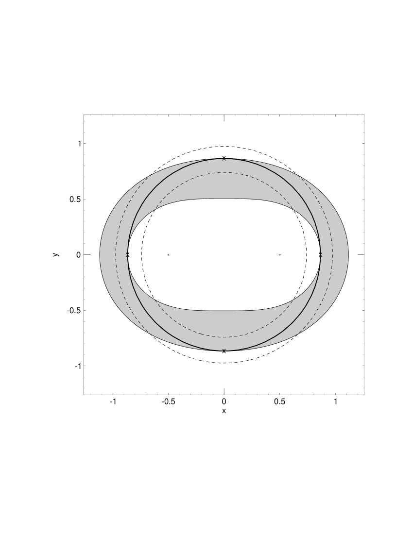
Figure 17: The approach to collapse. Initial positions available for the vortex with negative strength. The two vortex with strength $1$ are fixed, and located by the two thick points on the plot. Circles refer to different values of the constant $K$, while the oval curves correspond to different values of $\Lambda$. The shaded region corresponds to initial conditions leading to the aperiodic infinite expansion type of motion.

In the “resonant” case $k=1/2$, the critical circle represents a set of initial conditions leading to a self-similar collapse or expansion. Level lines of $\Lambda$ cross the circle in four points for $\Lambda\in(1/2,1)$, see Figure 17. These points are reflections of each other in the coordinate axes, this symmetry lead the coordinate axis to divide the plane in four dynamically equivalent quadrants. A reflection of a vortex configuration is equivalent to changing the direction of time, so that points in adjacent quadrants have opposite directions of their dynamics. From the original equations (8), we deduce, that the parts of the critical circle lying in the I and III quadrants lead to a finite-time collapse, and those in II and IV quadrants to an infinite self-similar expansion.

Four intersections of the critical circle with the coordinate axes are equilibrium positions, where $\Lambda$ reaches its limiting values (on the circle); the maximum value $\Lambda=1$ corresponds to the equilateral triangle, and the minimum $\Lambda=1/2$ to collinear configuration.

We define a rate of collapse as a rate of change of the squared distance between the two positive vortices, i.e. as $\dot{X}$. In this case, self-similar motion will have constant rate of collapse. Indeed, vortex velocities are inversely proportional to the inter-vortex distances, so that $\dot{X}=2R_{1}\dot{R}_{1}$ is independent of the scale of the motion. The rate of collapse is determined by the vortex energy:

$$\dot{X}(\Lambda)=\sqrt{4(1-\Lambda^{2})(1/4-\Lambda^{2})},$$ (49)

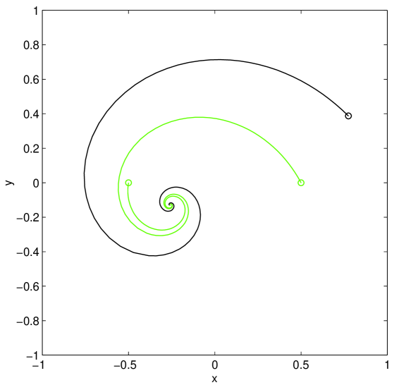
Figure 18: Vortex trajectories during collapse. Initial positions are shown by circles, they correspond to a fastest collapse value $\Lambda=\sqrt{3}/2$; negative vortex trajectory is plotted in black, positive ones in gray. All three vortices converge to the center of vorticity in finite time $\tau=4\pi/3$.

it tends to zero when $\Lambda$ approaches one of the equilibrium values $\Lambda=1/2,\>1$. Figure 18 shows vortex trajectories for the fastest collapse case $\Lambda=\sqrt{3}/2$.

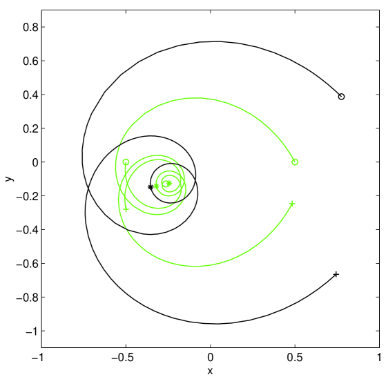
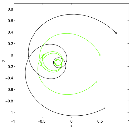
Figure 19: Unbounded near-collapse motion for $k=1/2$. Negative vortex: black; positive: gray. Closest approach positions are marked by asterisks.

When the negative vortex is slightly away from the critical circle, motion type depends on whether $\Lambda$ lies in the interval $(1/2,1)$ or not. If $\Lambda\in(1/2,1)$, vortices escape to infinity, their motion is aperiodic and unbounded. If the negative vortex lies in the I or III quadrant, vortex triangle starts to contract in a nearly self-similar way, resembling an exact collapse trajectory, but by the time when $X$ reaches its minimum value ($K/(1/2-\Lambda)$ for $K<0$ or $K/(1-\Lambda)$ for $K>0$) the triangle evolves into a collinear ($K<0$) or isosceles ($K>0$) configuration, as shown in Figure 19. After that vortices start to expand ad infinitum, asymptotically approaching a self-similar expanding trajectory. It follows, that a contracting self-similar motion in unstable, while an expanding one is asymptotically stable, a result obtained in [31] via linear analysis. When $\Lambda\notin[1/2,1]$ motion becomes periodic, $X$ oscillates in an interval $(K/(1-\Lambda);K/(1/2-\Lambda))$ for $K<0$ or $(K/(1/2-\Lambda);K/(1-\Lambda))$ for $K>0$.

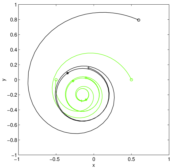
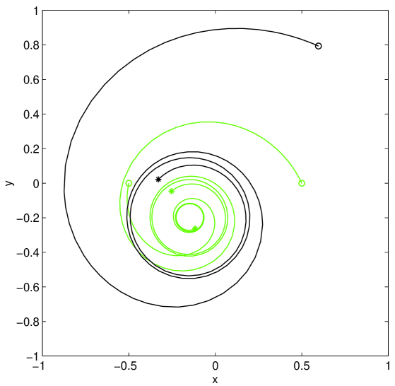
Figure 20: Motion in the vicinity of a saddle-point $\Lambda=\Lambda_{c_{2}}$ Contracting vortices approach an unstable equilibrium configuration, their spiral trajectories tighten and become nearly circular.

In case $k\neq 1/2$ unbounded motion does not exist anymore, yet the ratio of maximum vortex separation during the motion to the closest approach distance can be arbitrarily large as $k\rightarrow 1/2$. An interesting phenomenon is an existence of bounded aperiodic motions for particular values of vortex energy. They occur when an unstable equilibrium collinear configuration $X=X_{c_{2}}$ appears at $\Lambda=\Lambda_{c_{2}}$. Apart from the logarithmic divergence of the motion period near $\Lambda_{c_{2}}$ it also leads to a discontinuous dependence of the closest approach distance $X_{min}$ on initial vortex positions. Indeed, contracting vortices with $\Lambda=\Lambda_{c_{2}}-\epsilon$ where $\epsilon$ in an arbitrarily small positive number, will not pass through $X=X_{c_{2}}$, implying $X_{min}\approx X_{c_{2}}$, while infinitesimally different initial configuration with $\Lambda=\Lambda_{c_{2}}+\epsilon$ will, leading to further contraction. This is illustrated in Figure 20.

To resume, approaching collapse means taking the limits $K\rightarrow 0$ and $k\rightarrow 0.5$. These limits are not commutative, and for certain situations, the result depends on how the limits are taken, e.g. these limits may induce the divergence of $X_{c_{1,2}}$ or set them to zero or any value. Therefore a three vortex system can approach collapse in a number of different ways. For instance, if we take one limit after another, we can obtain the properties of the motion from the cases listed in Section 3.4 and Section 3.5. It is also interesting to study some of the scenarios, when the limits $K\rightarrow 0^{+-}$ and $k\rightarrow 0.5^{+-}$ are taken simultaneously, leading to an interplay of different situations, described in the previous Section. As an example, consider a limit $K\rightarrow 0^{+}$, $k\rightarrow 0.5^{-}$ taken along the line $K/\delta=C$, where $C$ is a constant. In this case, the saddle-point critical values $(X_{c_{2}},\Lambda_{c_{2}}$ tend to $(C,1/2)$, i.e. the scale of the inner potential well (bounded by $X_{c_{2}}$) stay the same. At the same time the outer potential well spreads two infinity, and we have a situation, when two types of motion, corresponding to the same value of vortex energy, have entirely different length scales.

5 Tracer advection near collapse

As we have mentioned, a prominent feature of near collapse dynamics is a generation of new length scales, which can differ from the length scale of the original configuration by orders of magnitude (see for instance (47)). This property has a strong influence on the mixing properties of the vortex flow. In this Section we display some preliminary results on the difference of the advection of passive particles (tracers) induced by collapse for a three-vortex system. We compare the motion of passive particles (tracers) in a velocity field of a near collapse configuration, with that in a typical “far from collapse” flow. A stream function of the flow, induced by moving vortices can be written as:

$$\psi(\textbf{x},t)=-\frac{1}{2\pi}\sum^{3}_{i=1}\ln|\textbf{x}-\textbf{x}_{i}(t)|$$ (50)

corresponding equations of tracer motion are:

$$\frac{d{\textbf{r}}(t)}{dt}={\textbf{e}}_{z}\wedge\nabla\psi$$ (51)

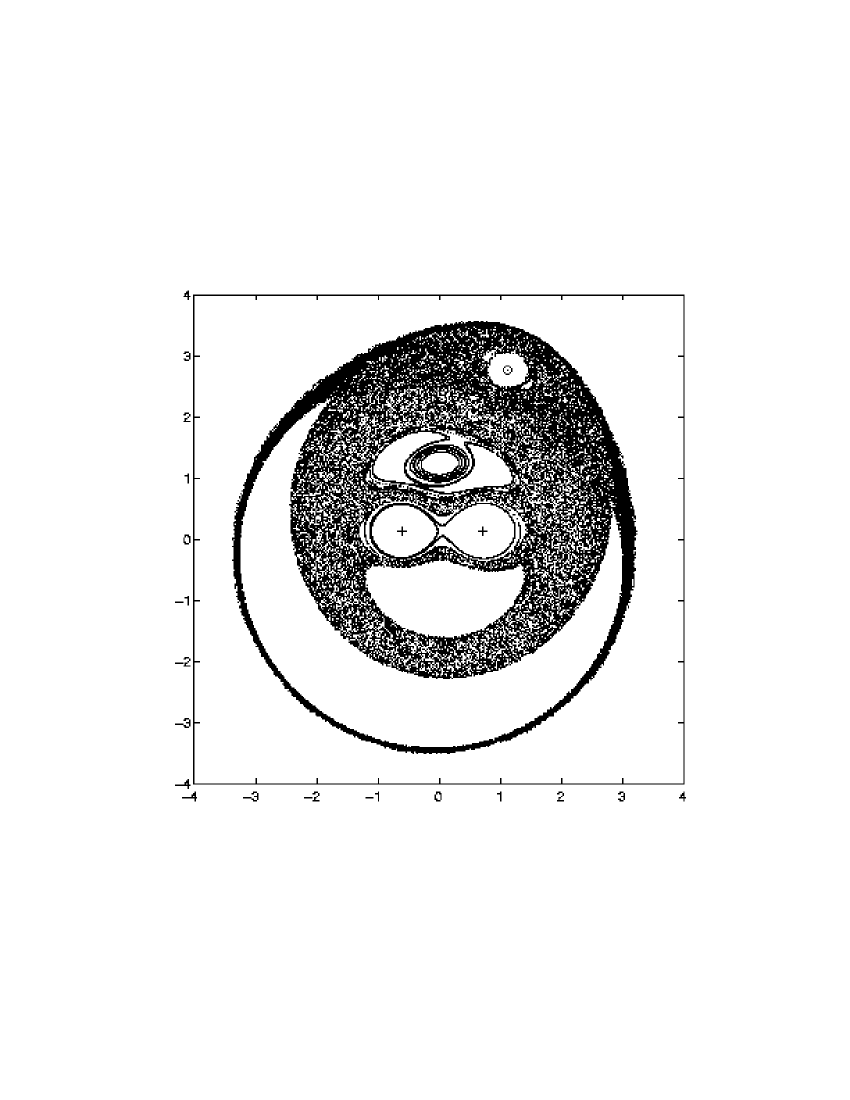
Figure 21: Far from collapse $\delta=0.4$. Poincar section of $253$ passive tracers in the flow field generated by three point vortex. The run is over $4000$ periods. The constant of motions are $\Lambda=0.9$, $K=0$. The vortex strengths are $(-0.1,\;1,\;1)$. The period of the motion is $T=6.59$.

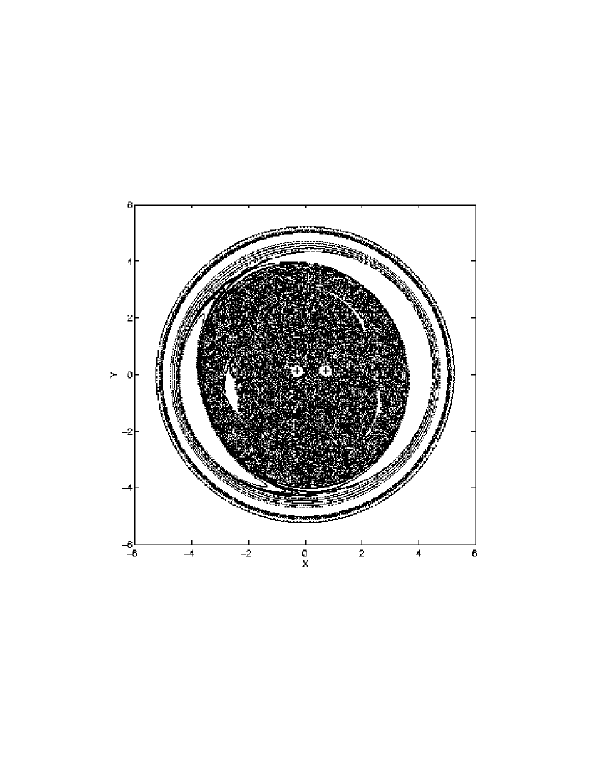
Figure 22: Far from collapse $\delta=0.09$. Poincar section of $253$ passive tracers in the flow field generated by three point vortex. The run is over $4000$ periods. The constant of motions are $\Lambda=0.9$, $K=0$. The vortex strengths are $(-0.41,\;1,\;1)$. The period of the motion is $T=36.86$.

where $\textbf{r}(t)$ denotes tracer position vector. Vortex trajectories $\textbf{x}_{i}(t)$ are periodic in a corotating reference frame, where (51) have a structure of a Hamiltonian system with $1\frac{1}{2}$ degrees of freedom [21, 36], so in a generic three-vortex flow some of the tracer trajectories are regular, and some are chaotic. To visualize advection patterns, we numerically construct Poincar section of tracer trajectories (in a corotating frame), which is an expedient tool for estimation of the degree of chaotization of advection, location of the main structures in the chaotic regions, etc. In Fig. 21, an example of an advection pattern of a far from collapse flow is presented. A large connected mixing region, regular cores around vortices, elliptic islands are typical elements of a tracer phase space in three-vortex flows [21, 36]. Two most important length scales in the advection pattern, associated with its robust features, are the outer radius of the mixing region and the radii of vortex cores. Generally, these two scales are comparable (their ratio is about one order of magnitude or less). However in advection patterns of near collapse vortex configurations, these length scales become considerably different, as the core radii tend to zero when approaching collapse see Fig. 22. The figures Fig. 21 and Fig. 22 are showed to emphasize that tracers chaotic dynamics in the near collapse case, is different than the dynamics without collapse. A more detailed analysis will be described in another article.

6 Conclusion

In this paper the behavior of a three point vortex system in a near collapse state was studied. We restricted ourselves to a special case where to vortex are identical which allowed the reduction of the system to an effective one dimensional Hamiltonian study. We were then able to classify all typical types of motion which could occur in a near collapse case, which qualitatively agrees with previous classification of the motion of three vortices [24][31] or collapse perturbations [29]. On the other hand our classification also focus on dynamical properties of the system, which are exhibited through the representation of trajectories in the effective phase space, giving us for example a direct insight on the period of the motion for the closed trajectories. It is in this sense complementary of the previous general classifications.

Furthermore, the singularity of the vortex collapse is special in the sense that near collapse dynamics shows a number of nontrivial dynamical features. In particular, the possibility of vorticity concentration allows one to speculate on the fact that the collapse situation exhibits some basics mechanisms which are of importance in $2D$ turbulence and its models. For instance, it becomes clear, that three-vortex collisions play an important role in the aggregation of vorticity in $2D$ turbulent flows, especially at the late stages of freely decaying turbulence, when the vorticity occupation is rather low [38]. Among these three-vortex collisions, near collapse ones are the more effective in bringing vortex together, and are thus the most important ones; this speculation is supported by the numerical simulations [28]. From this perspective, we give in this paper through the analysis of the effective potential, different typical length scales ($X_{c}$) and time scales (critical behaviors of the period), which shall be of importance in models attempting to describe $2D$ turbulence. For instance, the intricate structure of the vortex collapse singularity results in a very sensitive, non trivial dependence of the closest approach in the vicinity of collapse; it turns out that this is a discontinuous function of initial vortex positions. This is illustrated in Section 4, by the figure 20; in the same Section the configuration of the three vortices in their closest approach has also been discussed, and a clear distinction is made between the collinear and isoscele triangle configuration. These results could be of importance in deriving three-vortex merging rules analogous to the two-vortex ones used by current punctuated Hamiltonian models of $2D$ turbulence.

From the dynamical point of view, the study of vortex motion near the peculiar critical situation of collapse, has also revealed itself interesting in exhibiting a variety of behaviors. Namely, we observed for some situations different periodic motions for which critical behavior of the growth of the period with respect to the control parameter $\Lambda$ can be logarithmic, but it also can be as well a non-generic power-law growth with exponent $3/2$ (See Section 3.5 or Table 3). This last behavior is particular as in most cases, the approach of a singular critical point leads to a typical logarithmic divergence of the period, as for the near scattering situation discussed in [24].

Another motivation was how, the near-collapse dynamics influence the properties of passive particles. Advection in the chaotic region of the flow due to three identical vortices is superdiffusive [36]; tracers statistics is non-Gaussian, and is characterized by power law tails in the tracer probability density function, and algebraic decay of Poincar recurrences statistics; both are the consequences of the presence of long regular flights in a chaotic tracer trajectory. We expect the advection in a general three vortex system to be anomalous too, but the question whether or not the power law exponents and self similar behavior of the the tracer distribution observed in [39] are universal, remains open at the moment. With this in mind, it seems that the “extreme” dynamics encountered in near collapse dynamics, seem to be the most appropriate candidate to check if such universality exists. In this paper we limit ourselves to a short illustration of the advection patterns evolve as collapse is approached. We have observed , that as the system approaches collapse, the degree of chaotization increases: the chaotic region grows and the area of the regular island inside it shrinks. A more detailed study of the dynamical and statistical properties of the advection in near-collapse flows is currently under way, and will be presented elsewhere.

To conclude, we emphasize once again the fact, that near collapse dynamics comprises several types of motion. Their time and length scales differ considerably, depending on the way the collapse conditions are violated.

Appendix: Power-law divergence

From the effective Hamiltonian (22) the period of the motion in the case $k=1/2$ and for instance $K>0$ and $\Lambda<1/2$ (see Fig. 15) is then simply defined by

$$T=2\int^{X_{1}}_{X_{3}}\frac{dX}{\sqrt{-V(X)}}\>,$$ (52)

where $X_{1}$ and $X_{3}$ are defined in (45). To obtain the asymptotic expression of the period as $\Lambda\rightarrow 1/2^{-}$(where the $-$ sign refers that we are taking a right limit $\Lambda<0.5$), we use some simple equivalents, and write

$$T\sim 2\lambda^{-1/2}\int_{1}^{X_{1}}\frac{dX}{\sqrt{X_{1}/X-1}}\sim 4\lambda^{-1/2}X_{1}\>,$$ (53)

using the expression (45) for $X_{1}$ and (46) for $\lambda$, we obtain the asymptotic behavior of the period as a function of $\Lambda$ and $K$

$$T\sim K\sqrt{\frac{3}{2}}\left(\frac{1}{2}-\Lambda\right)^{-3/2}\>.$$ (54)

The period diverges as $(1/2-\Lambda)^{-3/2}$ when $\Lambda$ approaches the collapse value of $1/2$, and $K\neq 0$. Note that the period is linear in $K$.

Figure 1: Notation chosen for the problem

Figure 14: Evolution of the effective potential $V(X)$ in the singular case $k=1/2$ ($\delta=0$) within the energy range corresponding to possible collapse $\Lambda\in[1/2,1]$. We notice that unbounded motion occurs.

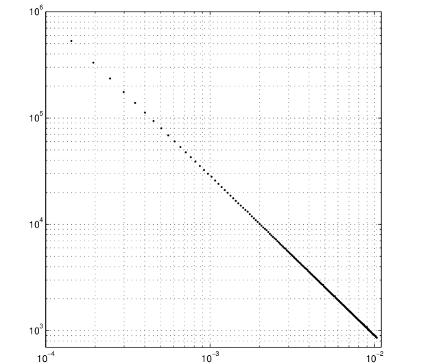
Figure 15: Period of the periodic motion ($\Lambda<1/2$) motion versus $|\Lambda-1/2|$ in the singular case $k=1/2$ ($\delta=0$). We notice a power-law divergence of the period as we approach collapse. The measured exponent is $3/2$. See appendix Appendix: Power-law divergence for the analytical computation.

Upper plot $K<0$: vortices contract until a collinear configuration with $X_{min}=K/(1/2-\Lambda)$ is reached.

Lower plot $K>0$: closest approach is this case is $X_{min}=K/(1-\Lambda)$ and corresponds to an isosceles triangle.

Upper plot $\Lambda<\Lambda_{c_{2}}$: vortex configuration cannot pass through the saddle-point, and reflects back after reaching collinear configuration.

Lower plot $\Lambda>\Lambda_{c_{2}}$: vortices “above” the saddle-point, and continue contraction (only a small piece of this part of the trajectory is shown).

References

- [1] P. Tabeling, A. E. Hansen, J. Paret, Forced and Decaying 2D turbulence: Experimental Study, in “Chaos, Kinetics and Nonlinear Dynamics in Fluids and Plasmas”, eds. Sadruddin Benkadda and George Zaslavsky, p. 145, (Springer 1998)
- [2] R. Benzi, G. Paladin, S. Patarnello, P. Santangelo and A. Vulpiani, Intermittency and coherent structures in two-dimensional turbulence, J. Phys A 19, 3771 (1986)
- [3] R. Benzi, S. Patarnello and P. Santangelo, Self-similar coherent structures in two-dimensional decaying turbulence, J. Phys A 21, 1221 (1988)
- [4] J. B. Weiss, J. C. McWilliams, Temporal scaling behavior of decaying two-dimensional turbulence, Phys. Fluids A 5, 608 (1992)
- [5] J. C. McWilliams, The emergence of isolated coherent vortices in turbulent flow, J. Fluid Mech. 146, 21 (1984)
- [6] J. C. McWilliams, The vortices of two-dimensional turbulence, J. Fluid Mech. 219, 361 (1990)
- [7] D. Elhmaïdi, A. Provenzale and A. Babiano, Elementary topology of two-dimensional turbulence from a Lagrangian viewpoint and single particle dispersion, J. Fluid Mech. 257, 533 (1993)
- [8] G. F. Carnevale, J. C. McWilliams, Y. Pomeau, J. B. Weiss and W. R. Young, Evolution of Vortex Statistics in Two-Dimensional Turbulence, Phys. Rev. Lett. 66, 2735 (1991)
- [9] N. J. Zabusky, J. C. McWilliams, A modulated point-vortex model for geostrophic, -plane dynamics, Phys. Fluids 25, 2175 (1982)
- [10] P. W. C. Vobseek, J. H. G. M. van Geffen,, V. V. Meleshko, G. J. F. van Heijst, Collapse interaction of finite-sized two-dimensional vortices, Phys. Fluids 9, 3315 (1997)
- [11] O. U. Velasco Fuentes, G. J. F. van Heijst, N. P. M. van Lipzig, Unsteady behaviour of a topography-modulated tripole, J. Fluid Mech. 307, 11 (1996)
- [12] R. Benzi, M. Colella, M. Briscolini, and P. Santangelo, A simple point vortex model for two-dimensional decaying turbulence, Phys. Fluids A 4, 1036 (1992)
- [13] J. B. Weiss, Punctuated Hamiltonian Models of Structired Turbulence, in Semi-Analytic Methods for the Navier-Stokes Equations, CRM Proc. Lecture Notes, 20, 109, (1999)
- [14] M. V. Melander, N.J. Zabusky, J.C. McWilliams, Phys. Fluids 30, 303 (1988)
- [15] I. Yasuda, G. R. Flierl, Two-dimensional asymmetric vortex merger: merger dynamics and critical merger distance, Dynam. Atmos. Oceans 26: (3) 159-181 OCT 1997
- [16] J. B. Weiss, A. Provenzale, J. C. McWilliams, Lagrangian dynamics in high-dimensional point-vortex systems, Phys. Fluids 10, 1929 (1998)
- [17] I. A. Min, I. Mezic, A. Leonard, Levy stable distributions for velocity difference in systems of vortex elements, Phys. Fluids 8, 1169 (1996)
- [18] V. V. Melezhko, M. Yu. Konstantinov, A. A. Gurzhi and T. P. Konovaljuk, Advection of a vortex pair atmosphere in a velocity field of point vortices, Phys. Fluids A 4, 2779 (1992)
- [19] A. Babiano, G. Boffetta, A. Provenzale and A. Vulpiani, Chaotic advection in point vortex models and two-dimensional turbulence, Phys. Fluids 6, 2465 (1994)
- [20] L. Zannetti and P. Franzese, Advection by a point vortex in a closed domain, Eur. J. Mech., B/Fluids 12, 43 (1993)
- [21] Z. Neufeld and T. Tél, The vortex dynamics analogue of the restricted three-body problem: advection in the field of three identical point vortices, J. Phys. A: Math. Gen. 30, 2263 (1997)
- [22] Z. Neufeld and T. Tél, Advection in chaotically time-dependent flow, Phys. Rev E 57, 2832 (1998)
- [23] G. Boffetta, A. Celani and P. Franzese, Trapping of passive tracers in a point vortex system, J. Phys. A: Math. Gen. 29, 3749 (1996)
- [24] H. Aref, Motion of three vortices, Phys. Fluids 22, 393 (1979)
- [25] E. A. Novikov, Yu. B. Sedov, Stochastic properties of a four-vortex system, Sov. Phys. JETP 48, 440 (1978)
- [26] H. Aref and N. Pomphrey, Integrable and chaotic motion of four vortices, Phys. Lett. A 78, 297 (1980)
- [27] S. L. Ziglin, Nonintegrability of a problem on the motion of four point vortices, Sov. Math. Dokl. 21, 296 (1980)
- [28] D. G. Dritschel, N. J. Zabusky, On the nature of the vortex interactions and models in unforced nearly-inviscid two-dimensional turbulence, Phys. Fluids 8(5), 1252 (1996)
- [29] E. A. Novikov, Yu. B. Sedov, Vortex collapse, Sov. Phys. JETP 22, 297 (1979)
- [30] J. L. Synge, On the motion of three vortices, Can. J. Math. 1, 257 (1949)
- [31] J. Tavantzis and L. Ting, The dynamics of three vortices revisited, Phys. Fluids 31, 1392 (1988)
- [32] Y. Kimura, Parametric motion of complex-time singularity toward real collapse, Physica D 46, 439 (1990)
- [33] C. Machioro and M. Pulvirenti, Mathematical theory of uncompressible nonviscous fluids, Applied Mathematical Science 96 (Springer-Verlag, New York, 1994)
- [34] P. Saffman, Vortex Dynamics, Cambridge Monographs on Mechanics and Applied Mathematics (Cambridge University Press, Cambridge, 1995)
- [35] H. Aref, Integrable, chaotic and turbulent vortex motion in two-dimensional flows, Ann. Rev. Fluid Mech. 15, 345 (1983)
- [36] L. Kuznetsov and G. M. Zaslavsky. Regular and Chaotic advection in the flow field of a three-vortex system. Phys. Rev E 58, 7330 (1998)
- [37] E. A. Novikov, Dynamics and statistics of a system of vortices, Sov. Phys. JETP 41, 937 (1975)
- [38] C. Sire and P. H. Chavanis, Numerical renormalization group of the vortex aggregation in 2D decaying turbulence: the role of three-body interactions. cond-mat/9912222 (1999)
- [39] L. Kuznetsov and G. M. Zaslavsky, Passive particle transport in three-vortex flow. To appear in Phys. Rev. E.