Bose-Einstein Condensation of Atomic Hydrogen

Abstract

This thesis describes the observation and study of Bose-Einstein condensation (BEC) of magnetically trapped atomic hydrogen. The sample is cooled by magnetic saddlepoint and radio frequency evaporation and is studied by laser spectroscopy of the $1S$-$2S$ transition in both the Doppler-free and Doppler-sensitive configuration. A cold collision frequency shift is exploited to infer the density of both the condensate and the non-condensed fraction of the sample. Condensates containing $10^{9}$ atoms are observed in trapped samples containing $5\times 10^{10}$ atoms. The small equilibrium condensate fractions are understood to arise from the very small repulsive interaction energy among the condensate atoms and the low evaporative cooling rate, both related to hydrogen’s anomalously small ground state $s$-wave scattering length. Loss from the condensate by dipolar spin-relaxation is counteracted by replenishment from the non-condensed portion of the sample, allowing condensates to exist more than $15$ s. A simple computer model of the degenerate system agrees well with the data. The large condensates and much larger thermal reservoirs should be very useful for the creation of bright coherent atomic beams. Several experiments to improve and utilize the condensates are suggested.

Attainment of BEC in hydrogen required application of the rf evaporation technique in order to overcome inefficiencies associated with one-dimensional evaporation over the magnetic field saddlepoint which confines the sample axially. The cryogenic apparatus (100 mK) had to be redesigned to accomodate the rf fields of many milligauss strength. This required the removal of good electrical conductors from the cell, and the use of a superfluid liquid helium jacket for heat transport. Measurements of heat transport and rf field strength are presented.

The rf fields in the apparatus allow rf ejection spectroscopy to be used to measure the trap minimum as well as the temperature of the sample.

Thesis Supervisor: Daniel Kleppner
Title: Lester Wolfe Professor of Physics

Thesis Supervisor: Thomas J. Greytak
Title: Professor of Physics

Chapter 1 Introduction

1.1 The Lure of Bose-Einstein Condensation

Bose-Einstein condensation (BEC) of a dilute gas has been a very important goal since the beginning of experimental research on spin-polarized atomic hydrogen. The original intent [1] was to study quantum phase transition behavior and search for superfluidity in this dilute gas, a weakly interacting system that is much more theoretically tractable than strongly interacting degenerate quantum systems such as superfluid liquid ⁴He. This phase transition is a purely quantum mechanical effect, and, unlike all other phase transitions, it occurs in the absence of any interparticle interactions.

Although the search for BEC in dilute gases began in spin-polarized hydrogen, the first observations of the effect used dilute gases of the alkali metal atoms Rb [2], Na [3], and Li [4, 5] in the summer of 1995. The properties of hydrogen that were so attractive in the beginning turned out, in the end, to be irrelevant or even a hindrance. Nevertheless, we have finally observed BEC in hydrogen [6, 7]. In several ways our hydrogen condensates are rather different from those of the alkalis, and we use different techniques to probe the sample. Hydrogen thus contributes significantly to the extraordinary flurry of experimental activity creating and probing Bose condensates, and applying them to intriguing new areas.

The formation of a Bose condensate out of a gas can be studied as the occurrence of a quantum mechanical phase transition, but perhaps even more interesting are the properties of the condensate itself. Centered in the middle of a trapped gas, this collection of atoms exhibits such bizarre effects as a vanishingly small kinetic energy, long range coherence across the condensate [8], a single macroscopic quantum state, immiscibilty of two components of a gas [9, 10], and constructive/destructive interference between atoms that have fallen many millimeters out of the cloud [11]. These systems hold promise for creating quantum entanglement of huge numbers of atoms for use in quantum computing and vastly improved fundamental measurements.

1.2 The Significance of the Work in this Thesis

In this thesis we describe the culmination of a 22 year research effort: the first observations of BEC in hydrogen. Furthermore, we demonstrate a new technique of probing Bose condensates, optical spectroscopy. This tool allows us to measure the density and momentum distributions of the sample, and thus infer the temperature, size of the condensate, and other properties. We find that the condensates we create contain nearly two orders of magnitude more atoms than other BEC systems, and the condensates occupy a much larger volume. In addition, we find that nearly $10^{10}$ atoms are condensed during the 10 s lifetime of the condensate. This high flux of condensate atoms implies that this system might be ideal for creation of bright, coherent atomic beams. Indeed, hydrogen has proven to be a rich and promising atom for further studies of BEC.

The thesis is divided as follows. Chapter 2 and the associated appendices provide a detailed description of the behavior of the trapped gas both in the classical and quantum mechanical regimes. Results are obtained to guide the reader’s intuition throughout the remainder of the thesis. Chapter 3 describes changes to the apparatus that allowed BEC to be achieved. Chapter 4 details use of the new capabilities of the improved apparatus. The most important contributions described in this thesis are found in chapter 5 where studies of BEC are presented. Finally, conclusions and suggestions for future work are made in chapter 6.

Much of the work described here was done in close collaboration with a group of people, as shown by the several names on our papers. In particular, this thesis should be considered a companion thesis to that of Thomas Killian [13]. Both should be read to obtain a complete picture of the whole experiment. The work builds on earlier work by Claudio Cesar, whose thesis [14] describes the first $1S$-$2S$ spectroscopy of trapped atomic hydrogen; Albert Yu, whose thesis [15] on universal quantum reflection includes important insights into non-ergodic atomic motion in the trap; Jon Sandberg, whose thesis [16] describes the physics of $1S$-$2S$ spectroscopy in a trap and the development of the uv laser system we use; and John Doyle, whose thesis [17] describes trapping and cooling of spin-polarized hydrogen and the magnet system we use to trap the gas.

1.3 The Basics of Trapping and Cooling Hydrogen

There is a long and interesting history of spin-polarized hydrogen in the laboratory, summarized well by Greytak [18]. Here we briefly summarize our method of creating spin-polarized hydrogen, loading it into a trap, and cooling it to BEC (quantum degeneracy). A broader description is in the thesis of Killian [13].

Hydrogen is composed of a proton and electron, whose spins can couple in four ways: the four hyperfine states are labeled $a$-$d$ (these states are derived in section 3.1.1). The high-field seeking states ($a$ and $b$) are pulled toward regions of high magnetic field, and the low-field seeking states ($c$ and $d$) are expelled from high field regions. Figure 1-1 shows the energies of the four states as a function of field strength.

Figure 1-1: Hyperfine-Zeeman diagram of ground state atomic hydrogen. The eigenstates of the combined hyperfine and Zeeman Hamiltonian are described in section 3.1. Atoms in states $c$ and $d$ can be trapped in a magnetic field minimum.

Our experiments use the pure, doubly-polarized $d$-state.

At the beginning of an experimental run molecular hydrogen is loaded into the cryogenic apparatus by blowing a mixture of H₂ and ⁴He into a cold ($T\simeq 1$ K) can, called the dissociator, where it freezes. Then, for each loading of the trap, H₂ molecules are dissociated by pulsing an rf discharge (the dissociator is in a region of high magnetic field, 4 T). The low field seekers are blown into a confinement cell (4 cm diameter, 60 cm length), over which the inhomogeneous trapping field is superimposed. The trap fields are created by currents in superconducting coils, described by Doyle [17] and Sandberg [16]. The coils create a trap with maximum depth 0.82 T, which, for hydrogen’s magnetic moment of 1 Bohr magneton, corresponds to an energy ${\epsilon_{t}}/{k_{B}}=550$ mK. (See appendix I for conversions between various manifestations of energy in this experiment.) The trap depth is the difference between the field at the walls of the containment cell and the minimum field in the middle of the cell. There are seventeen independently controlled coils in the apparatus which are used to adjust the trap shape. Figure 1-2 is a cutaway diagram of the system.

Figure 1-2: Cutaway view of apparatus. Molecular hydrogen is dissociated in an rf discharge in a 4 tesla region. The atoms move into the confinement cell which has superimposed on it a trap, created by the quadrupole coils (radial confinement) and the pinch coils (axial confinement). The coils are bathed in 4.2 K liquid helium. The cell is centered in the vacuum can with three Kevlar strings. It is thermally anchored to the mixing chamber of a dilution refrigerator (not shown). The laser beam passes through the upper window, retroreflects on the mirror at the bottom of the cell, and exits through the upper window. Atomic fluorescence photons pass through the MgF window and Lyman-$\alpha$ filter, and are counted on the microchannel plate detector.

Expanded views of the top and bottom of the cell are in figures 3-8 and 3-9. The trap shape used for capturing the atoms is basically a long trough. The field increases linearly away from the $z$ axis of the trap (the potential exhibits near cylindrical symmetry about the $z$ axis); the potential is small and roughly uniform for about 20 cm along the $z$ axis. “Pinch” coils at each end provide the axial confinement. The field profile indicated in figure 1-2 is along the $z$ axis of the cell.

The trap depth sets an energy scale: for atoms to be trapped their total energy must be less than the trap depth. Two techniques are used to cool the atoms into the trap. First, after H₂ molecules are dissociated [17, 19] the hot atoms are thermalized on the walls of the cell, held at 275 mK. In order to prevent the atoms from sticking tightly to the cold surfaces, a superfluid ⁴He film covers the walls and reduces the binding energy of the H atoms to a manageable $1.0$ K [20, 21, 22]. When the atoms leave the wall their total energy ($3{k_{B}}T/2$ of kinetic energy and ${\epsilon_{t}}$ of potential energy) is still greater than the trap depth. The second stage of cooling into the trap involves collisions among the atoms that are crossing the trapping region. Sometimes these collisions result in one atom having low enough energy to become trapped. The partner atom in the collision goes to the wall and is thermalized. The gas densities expected in the cell correspond to a collision length many times greater than the cell diameter, so atoms pass through the trapping region many times before becoming trapped. A recent study of the trap loading process will be published elsewhere [19].

After loading the trap, the cell walls are quickly cooled to below 150 mK to thermally disconnect the sample from the confinement cell. At these lower temperatures the residence time of an atom on the surface of the cell becomes much longer than the characteristic H+H$\rightarrow$ H₂ recombination time, and so the surface is “sticky”; all the atoms that reach the surface recombine before having a chance to leave the surface. Thermal disconnect between the cryogenic cell and the trapped sample is achieved because no warm particles can leave the walls and carry energy to the trapped gas. Atoms can leave the trapped gas and reach the wall, however, if they have large enough total energy to climb the magnetic hill. As these very energetic atoms irreversibly leave the trapped sample, it cools. In fact, this preferential removal of the most energetic atoms, called evaporation, is very useful. It is the cooling mechanism we exploit to create samples as cold as $20~{}\mu$K, as described in chapter 5. A thorough description of the heating and cooling processes which set the temperature of the system is found in appendix A.

We catch both the $d$ and $c$ low field seeking states in the trap. However, inelastic collision processes involving two $c$ state atoms quickly deplete the $c$-state population, and the remaining atoms constitute a doubly polarized sample (both electron and proton spins are polarized). Because the spin state is pure, the spin-relaxation rate is rather small. For peak densities in the normal gas of $n\simeq 10^{14}~{}{\rm cm}^{-3}$ (nearly the largest for these experiments) the characteristic decay time is 40 s.

The trapped gas is probed using various techniques. The simplest method involves quickly lowering the magnetic confinement barrier at one end of the trap, and measuring the flux of escaping atoms as a function of barrier height [17, 23]. In a limited regime this technique can be used to infer the gas temperature and density. This technique, and its limitations, is described in chapter 4. Another technique is rf ejection spectroscopy, described in chapter 4. The third probe technique is laser spectroscopy of the $1S$-$2S$ transition, envisioned [24, 16], realized [14, 25], and perfected [13] in our lab for a trapped gas. This diagnostic tool can give the density and temperature of the gas over a wider range of operating conditions than the other techniques, and has proven crucial for studies of BEC. The laser probe will be described in more detail in chapter 5, and is a principle subject of the companion thesis by Killian [13].

Chapter 2 Theoretical Considerations

This chapter addresses two important topics from a theoretical perspective. First, we explain why previous experiments could not bring trapped hydrogen into the quantum degenerate regime. This understanding allowed us to solve the problem and achieve BEC. The second topic is related to the small fraction (only a few percent) of atoms we are able to put into the condensate. This situation differs markedly from that observed in Rb and Na BEC experiments. An explanation of this difference and others is the second topic we explore theoretically.

The starting point for understanding the behavior of the trapped gas is classical statistical mechanics. Good explanations have been developed elsewhere [26, 27, 17, 28]. For completeness, we present a development in appendix A. Since the gas exists in a trap of finite depth ${\epsilon_{t}}$, we use a truncated Maxwell-Boltzmann occupation function. Knowledge of the trap shape allows us to calculate the population, total energy, density, etc. The effects of truncation of the energy distribution at the trap depth are included in these derivations. We see that for deep traps ($\eta\equiv{\epsilon_{t}}/{k_{B}}T>7$) the truncation does not significantly alter the properties of the system from estimates based on an untruncated distribution. Appendix A also explains the density of states functions (see section A.1.2) used in the remainder of the thesis and summarizes evaporative cooling (see section A.2).

2.1 Dimensionality of Evaporation

The temperature of the gas is set by a balance between heating and cooling processes, as described in section A.2.2. Previous attempts to attain BEC in hydrogen [29, 30] failed because the cooling process became bottlenecked by the slow rate at which energetic atoms could escape, thus reducing the effective cooling rate. To understand this bottleneck we must first consider the details of the trap shape. We then study the motion of the particles that have enough energy to escape.

The trap shape used to confine samples at $T<200~{}\mu$K is often called the “Ioffe-Pritchard” [31, 26] type (labeled “IP”). Using axial coordinate $z$ and radial coordinate $\rho$, the potential has the form

$$V_{IP}(\rho,z)=\sqrt{(\alpha\rho)^{2}+(\beta z^{2}+\theta)^{2}}-\theta$$ (2.1)

with radial potential energy gradient $\alpha$ (units energy/length), axial potential energy curvature $2\beta$ (units of energy/length²), and bias potential energy $\theta$. See section A.1.2 for a summary of the density of states functions for this trap.

In the limit of $\rho\ll\theta/\alpha$, the Ioffe-Pritchard potential is harmonic in the radial coordinate, as may be seen by expanding the potential in powers of $\alpha\rho/(\beta z^{2}+\theta)$:

$$V_{IP}(\rho,z)=\beta z^{2}+\frac{1}{2}\frac{\alpha^{2}}{\beta z^{2}+\theta}\>\rho^{2}\;+\;\frac{1}{8}\>\frac{\alpha^{3}}{(\beta z^{2}+\theta)^{2}}\>\rho^{3}\;+\cdots.$$ (2.2)

The trap is harmonic in the radial direction when the third term is much smaller than the second term. This is true for radial coordinates $\rho\ll\rho_{anharm}$, where we have defined the “anharmonic radius” at which the second term matches the third term:

$$\rho_{anharm}\equiv 4\>\frac{\beta z^{2}+\theta}{\alpha}.$$ (2.3)

The trap appears harmonic in all three directions to short samples for which the radial oscillation frequency is essentially uniform along the length of the sample. This occurs for temperatures $T\ll 4\theta/{k_{B}}$. In the harmonic regime, the axial oscillation frequency is

$$\omega_{z}=\sqrt{\frac{2\beta}{m}},$$ (2.4)

and the radial oscillation frequency is

$$\omega_{\rho}=\alpha\sqrt{\frac{m}{\beta z^{2}+\theta}}.$$ (2.5)

For the evaporation to proceed efficiently, atoms with energy greater than the trap depth ${\epsilon_{t}}$ (called “energetic atoms”) must leave the trap promptly, before having a collision. As shown in appendix B, in the vast majority of cases an energetic atom that collides with a trapped atom will become trapped again. The rare collision that produced the energetic atom will be “wasted”. It is essential to understand the details of the particle removal process if maximum evaporation efficiency is to be achieved.

Previous attempts to cool hydrogen to BEC utilized “saddlepoint evaporation”, in which energetic atoms escape over a saddlepoint in the magnetic field barrier at one end of the trap. To escape, the atom must have energy in the axial degree of freedom ($z$) that is greater than ${\epsilon_{t}}$. This atom removal technique is inherently one dimensional. The collisions which drive evaporation produce many atoms with high energy in the radial degrees of freedom, and in order for these to escape the energy must be transferred to the axial degree of freedom. This energy transfer process was analyzed theoretically by Surkov, Walraven, and Shlyapnikov [32], and we follow their analysis.

In a harmonic trap the potential is separable, and the particle motion is completely regular; no energy exchange occurs. In the Ioffe-Pritchard trap, however, energy exchange can occur because the potential is not separable; the radial oscillation frequency depends on the axial coordinate, $z$, and so radial motion can couple to axial motion. (See equation 2.5.)

This energy mixing can be understood by considering how rapidly the radial oscillation frequency changes as an atom moves along the $z$ axis. If the frequency changes slowly (“adiabatically”), then the energy will not mix among the degrees of freedom. The adiabaticity parameter is the fractional change of the radial oscillation frequency in one oscillation period as the atom moves axially through the trap. Strong mixing occurs when

$$\frac{\dot{\omega}_{\rho}}{\omega_{\rho}^{2}}\sim 1.$$ (2.6)

Here $\dot{\omega}_{\rho}=(d\omega_{\rho}/dz)(dz/dt)$. For a Ioffe-Pritchard trap with a bias that is large compared to ${k_{B}}T$, $\omega_{\rho}=\alpha/\sqrt{(\beta z^{2}+\theta)m}$. We have used the expansion of $V_{IP}$ from equation 2.2, which is valid if ${k_{B}}T\sim\alpha\rho\ll\theta$. Given that ${k_{B}}T\ll\theta$, the adiabaticity parameter is

$$\frac{\dot{\omega}_{\rho}}{\omega^{2}_{\rho}}=v_{z}\>\frac{\beta z\sqrt{m}}{\alpha\sqrt{\beta z^{2}+\theta}}.$$ (2.7)

We see that several factors contribute to good mixing: large axial velocity $v_{z}$ (which occurs at high temperature), small radial gradient $\alpha$, small bias field $\theta$, and large axial curvature $\beta$. In practice, however, achieving BEC requires low temperatures ($v_{z}$ small) and high densities (obtained with large compressions, and thus large $\alpha$). Consequently, the degrees of freedom do not mix and evaporation becomes essentially one dimensional. Typical values for our experiment are $\alpha/{k_{B}}=16~{}{\rm mK}/{\rm cm}$, $\beta/{k_{B}}=25~{}\mu{\rm K}/{\rm cm^{2}}$, $\theta/{k_{B}}=30~{}\mu{\rm K}$, $T=100~{}\mu{\rm K}$, $z\sim 2~{}{\rm cm}$, and $v_{z}=140~{}{\rm cm}/{\rm s}$, so that $\dot{\omega_{\rho}}/\omega_{\rho}^{2}\sim 10^{-3}$. For these conditions it takes about $10^{3}$ oscillations to transfer energy, but there are only about $\omega_{\rho}/2\pi\Gamma_{col}\sim 200$ oscillations per collision for a peak sample density $n_{0}=10^{14}~{}{\rm cm}^{-3}$ ($\Gamma_{col}$ is the elastic collision rate, pA.2). There is not enough time to transfer the radial energy to axial energy before the particle has a collision. The energy mixing is thus very weak and the evaporation is one dimensional. Surkov et al. [32] pointed out the consequences of one-dimensional evaporation. They estimated that the efficiency is reduced by a factor of $4\eta$ compared to that of full 3D evaporation. The evaporative cooling power thus drops dramatically. Experiments in our laboratory (unpublished) have confirmed that phase space compression ceases near $100~{}\mu$K. These results were duplicated and studied in more depth by Pinkse et al. [30].

In order to maintain the evaporation efficiency a technique is required that quickly removes all particles with energy greater than the trap depth. To this end we implemented rf evaporation, as described in detail in chapter 3.

2.2 Degenerate Bose Gas

2.2.1 Bose Distribution

The statistical mechanical description of a classical gas, presented in appendix A, is not correct when quantum effects are important. A simple way to understand the crossover to the quantum regime is to recall that particles are characterized by wavepackets whose size is related to their momentum by the Heisenberg momentum-position uncertainty relation. As a gas is cooled, the particle momenta decrease, and the wavepackets enlarge. The classical (point-particle) description of the system breaks down when these wavepackets begin to overlap. The quantum treatment correctly deals with the effect of particle indistinguishability. There are many excellent treatments of quantum statistical mechanics [33]. Here we review the basic features that are important for our experiment.

A collection of identical particles with integer (half-integer) spins must have a total wavefunction that is symmetric (anti-symmetric) when two particles are exchanged. The connection between spin and symmetry has been explained using relativistic quantum field theory [34]. Particles with integer (half-integer) spin are called bosons (fermions). In contrast to fermions, multiple bosons may occupy a single quantum state.

The occupation function for a gas of $N$ identical bosons in a box of volume $V$, and in the limit of $N\rightarrow\infty$ and $V\rightarrow\infty$ but constant $N/V$, is called the Bose-Einstein occupation function [33]

$$f_{BE}(\epsilon)=\frac{1}{\exp^{(\epsilon-\mu)/{k_{B}}T}-1},$$ (2.8)

where $\mu$ and $T$ are Lagrange multipliers which constrain the system to exhibit the correct population and total energy through the conditions

$$\frac{N}{V}=\int d\epsilon\;\frac{\rho(\epsilon)}{V}\>f_{BE}(\epsilon)$$ (2.9)

and

$$\frac{E}{V}=\int d\epsilon\;\epsilon\>\frac{\rho(\epsilon)}{V}\>f_{BE}(\epsilon).$$ (2.10)

The physical interpretation of these parameters is that $\mu$ is the chemical potential and $T$ is the temperature. Figure 2-1

Figure 2-1: Comparison of Maxwell-Boltzmann (dashed line) and Bose-Einstein (solid line) distributions of particle energies, plotted for various chemical potentials. The peak density, a quantity related to the onset of BEC and to evaporation and decay rates, is identical for each pair of curves. The vertical axis is the number of atoms with the given energy. This is proportional to the occupation function weighted by the total energy density of states for a Ioffe-Pritchard trap, $\propto\epsilon^{3}+2\theta\epsilon^{2}$. Here $\theta/{k_{B}}T=1$.

shows the energy distribution of the population in the trap for a classical gas described by the Maxwell-Boltzmann (MB) distribution and for a quantum gas described by the Bose-Einstein (BE) distribution. The two functions shown describe systems with identical peak densities, a parameter relevant to the creation of a condensate. The MB distribution requires many more particles than the BE to create the same peak density because the atoms are distributed at higher energies, further from the center of the trap.

The difference between the BE and MB distributions originates in the different assumptions about particle distinguishability. To intuitively understand this, we consider the outcome of these differing assumptions for sparsely and densely occupied sets of energy states. In the classical treatment there are many ways to arrange the distinguishable particles among sparsely occupied energy states because interchanging any pair of particles leads to a different arrangement. For very densely occupied states, interchanges of distinguishable particles often result in the same arrangement because the particles often do not change energy level. For a collection of distinguishable particles with a given total energy, there are “extra” arrangements in which the particles are sparsely distributed. In contrast, for indistinguishable particles any interchange of two particles results in the same overall arrangement of particles, regardless of whether the states are sparsely or densely occupied. There are thus no “extra” sparse arrangements of particles.

In a gas near the quantum degenerate regime the occupation of the energy levels ranges from dense ($\sim 1$ at low energies) to sparse ($\ll 1$ at high energies). Using the assumption of equal a priori probabilities [33], distinguishable particles will most likely be found in those arrangements with the more sparse level occupations (higher overall energies) because there are so many more of these arrangements. Indistinguishable particles give no rise to such “extra” arrangements, and so the most likely arrangements will involve more dense level occupations (lower overall energies) than predicted by classical theory. Figure 2-1 demonstrates this effect. For each pair of curves the peak density, $n_{0}$, is identical. The peak density is the experimentally observable quantity. Since the MB occupation function favors arrangements with higher energy (and thus atoms are distributed over a larger volume in the trap), more atoms are required in the sample to produce the same peak density. The curves thus do not exhibit equal area.

Bose-Einstein condensation occurs when the chemical potential goes to zero and the occupation of the lowest energy state diverges. This occurs at the critical density [33]

$$n_{c}=g_{3/2}(1)/\Lambda^{3}(T)$$ (2.11)

where $g_{n}(z)\equiv\sum_{l=1}^{\infty}z^{l}/l^{n}$; $g_{3/2}(1)=2.612$. A gas that has undergone the Bose-Einstein phase transition is said to be in the quantum degenerate regime because a macroscopic fraction of the particles are in an identical quantum state.

Although a hydrogen atom consists of two fermions, it behaves like a composite boson for the studies in this thesis because the collision interaction energies are extremely small compared to the electron-proton binding energy [35]. The two fermions act as a unit except in high energy collisions where electron exchange is possible. The typical interaction energy during low temperature collisions is $\sim 1$ mK, which corresponds to $10^{-7}$ eV, $10^{8}$ times smaller than the binding energy.

To analyze the behavior of the degenerate Bose gas we shall separately treat the condensed and non-condensed portions of the system. The condensate is treated in section 2.2.2. The non-condensed fraction, which we call the “normal gas” or “thermal gas”, is treated in appendix C. The results derived here will be used to understand how the hydrogen system is different from other gases that have been Bose condensed (section 2.3), and to interpret the experimental results in chapter 5 (note that truncation effects are important because of the shallow traps used for those experiments, $4<\eta<6$).

2.2.2 Description of the Condensate

2.2.2.1 Gross-Pitaevskii Equation

When Bose-Einstein condensation occurs, a macroscopic fraction of the particles occupy the lowest energy quantum state of the system, and thus have the same wavefunction. For a non-interacting Bose gas, that wavefunction is simply the lowest harmonic oscillator wavefunction for the trap. Interactions become important when many particles occupy this region of space and the local density increases. In this case the wavefunction spreads out due to repulsion among the atoms. There is a large body of literature on Bose-Einstein condensates (see [36] for a recent review), and so we simply quote here the most important results.

The Schroedinger equation for the interacting condensate is called the Gross-Pitaevskii equation [37, 38, 39], and has the form

$$-\frac{\hbar^{2}}{2m}\nabla^{2}\psi({\bf r})+V({\bf r})\psi({\bf r})+U_{0}\left|\psi({\bf r})\right|^{2}\psi({\bf r})=\mu\psi({\bf r})$$ (2.12)

where $\psi({\bf r})$ is the condensate wavefunction to be determined. The eigenenergy of the wavefunction is $\mu$, which is the total energy of each condensate atom. The quantity $U_{0}\equiv 4\pi\hbar^{2}a/m$ parameterizes the mean field energy, which is the energy of interaction among the atoms per unit density, and is repulsive for $s$-wave scattering lengths $a>0$. For hydrogen in the ground state, $a=0.648~{}{\rm\AA}$[40], and $U_{0}/{k_{B}}=3.92\times 10^{-16}~{}\mu{\rm K~{}cm}^{3}$. The mean field energy augments the trap potential by an amount proportional to the local condensate density $n_{cond}({\bf r})=\left|\psi({\bf r})\right|^{2}$. Note that interactions between the condensate and non-condensed atoms are neglected here. For the experiments in this thesis, this interaction energy is small because the density of non-condensed atoms (called the “thermal gas” or “normal gas”) is small. Furthermore, the interaction energy with the thermal gas is essentially uniform across the condensate because the density of non-condensed atoms varies only weakly; the thermal energy of the normal gas ($T_{c}\sim 60~{}\mu$K) is much larger than the condensate mean field energy ($\mu/{k_{B}}\sim 2~{}\mu$K), and thus the density of the normal gas does not change appreciably on the length scale of the condensate.

We identify the eigenenergy $\mu$ in equation 2.12 with the chemical potential of the system in equilibrium. The chemical potential is the energy required to add a particle to the system. When a condensate is present, the normal gas is “saturated”, and any particles added to the system go into the condensate. The energy required to add the last atom to the condensate is $\mu$, the eigenenergy, and so we link $\mu$ with the chemical potential. In practice we measure $\mu$ spectroscopically through the peak density at the center of the condensate, which is in turn measured through the cold-collision frequency shift. This is explained in section 5.3.1.

2.2.2.2 Thomas-Fermi Approximation

If the condensate density is large enough so that the mean field energy is much greater than the kinetic energy of the wavefunction, then the kinetic energy term (also called the quantum pressure term) in equation 2.12 may be neglected. Using this “Thomas-Fermi” approximation we obtain the condensate density profile

$$n_{cond}({\bf r})=n_{p}-V({\bf r})/U_{0}$$ (2.13)

where $n_{p}\equiv\mu/U_{0}$ is the peak condensate density (the largest density in the condensate, found at the bottom of the trap). The Thomas-Fermi approximation is valid over most of the volume of the condensate, but near the edges the condensate density approaches zero, and the kinetic energy term should be included. We ignore this small correction in the calculations which follow because it is minor for interpretation of the experiments described in this thesis. See [41] for a good description of various ways to go beyond the Thomas-Fermi approximation.

The condensate density profile may be obtained without the Gross-Pitaevskii equation by assuming the condensate is stationary and its particles are at rest, and then balancing hydrodynamic forces [42]. A condensate particle in a region of potential energy $\varepsilon$ has total energy $E=\varepsilon+n_{cond}(\varepsilon)U_{0}$. Since there must be no net force on the particle, $E={\rm const}\equiv n_{p}U_{0}$ and $n_{cond}(\varepsilon)=n_{p}-\varepsilon/U_{0}$.

2.2.2.3 Population and Loss Rate

The population of the condensate is easily computed using the Thomas-Fermi wavefunction in the bottom of the IP trap, which is parabolic for the condensate sizes and trap parameters of interest in this thesis. We approximate the potential energy density of states (see pA.1.2) as $\varrho(\varepsilon)\approx{\cal A}_{IP}\sqrt{\varepsilon}\theta$ and obtain

$$N_{c} = \int_{0}^{U_{0}n_{p}}d\varepsilon\;{\cal A}_{IP}\>\theta\sqrt{\varepsilon}(n_{p}-\varepsilon/U_{0})$$ (2.14)

$$= \frac{4}{15}{\cal A}_{IP}\>\theta\>U_{0}^{3/2}n_{p}^{5/2}.$$

As noted above, the total energy of each condensate atom is the chemical potential $\mu=n_{p}U_{0}$, so $E_{c}=\mu N_{c}$.

The loss rate from the condensate due to two-body dipolar relaxation is found by integrating the square of the density over the volume of the condensate:

$$\dot{N}_{2,c} = -\int_{0}^{U_{0}n_{p}}d\varepsilon\;{\cal A}_{IP}\>\theta\sqrt{\varepsilon}\>(g/2!)\>(n_{p}-\varepsilon/U_{0})^{2}$$ (2.15)

$$= -\frac{16}{105}\>\frac{g}{2!}{\cal A}_{IP}\theta\>U_{0}^{3/2}n_{p}^{7/2}$$

where the $2!$ accounts for correlation properties of the condensate [43, 44]. Here the dipolar decay rate constant $g$ is slightly different from that given in equation A.19 because the rate constant $G_{dd\rightarrow cd}$ should be multiplied by 2; the energy $\theta$ liberated in this process is large compared to $\mu$. This term is small, so $g$ is not effected much. The energy loss rate is $\dot{E}_{2,c}=\mu\dot{N}_{2,c}$. The characteristic condensate decay rate in a parabolic trap is

$$-\frac{\dot{N}_{2,c}}{N_{c}}=\frac{2}{7}gn_{p},$$ (2.16)

which is $1.6~{}{\rm s}^{-1}$ for a typical peak density $n_{p}=5\times 10^{15}~{}{\rm cm}^{-3}$.

2.3 Properties of a Bose-Condensed Gas of Hydrogen

Hydrogen differs in several ways from alkali metal atoms that have been Bose condensed. The principal differences are its small mass and small $s$-wave scattering length. How do these properties influence the system?

First, the small mass implies that BEC occurs at a higher temperature for a given peak density: from equation 2.11, $T_{c}\propto 1/m$. We have observed the transition at temperatures roughly 50 times higher than in the other systems.

Further, as estimated by Hijmans et al. [45] and will be shown in the following sections, the maximum equilibrium condensate fraction is small for hydrogen. This will be explained by noting the relatively high density of the condensate, as compared to the thermal cloud. This high density leads to high losses through dipolar decay, which result in heating of the system. This heating must be balanced by evaporative cooling, which proceeds slowly in hydrogen because of the small collision cross section. The result of these factors is that only small condensate fractions are possible in equilibrium. Possible remedies will be noted.

Finally, hydrogen’s small collision cross-section should allow condensates of H to be produced by evaporative cooling that contain many orders of magnitude more atoms than those possible in alkali-metal species, as explained in the section 2.3.4.

2.3.1 Relative Condensate Density

For trapped hydrogen, the condensate density grows much greater than the density of the non-condensed portion of the gas at even very small condensate fractions [18], a distinct difference from other species that have been Bose-condensed. This is noteworthy for possible future studies of behavior near the phase transition. As shown in section 2.3.2, it also has implications for the maximum condensate fraction that may be achieved in hydrogen. In this section we calculate the ratio of the densities as a function of the condensate fraction. We compare hydrogen to Li, Na, and Rb.

The condensate fraction is

$$F\equiv\frac{N_{c}}{N_{c}+N_{t}}$$ (2.17)

where the population of the thermal cloud, $N_{t}$, is found using equation C.7 and the population of the condensate is given by equation 2.14. The fraction can be written in terms of the more convenient population ratio, $f\equiv N_{c}/N_{t}$, as $F=f/(1+f)$. For a given peak condensate density, sample temperature, and set of trap parameters, the population ratio is

$$f=\underbrace{\left(\frac{2^{7/2}h^{6}a^{3/2}}{\pi^{7/2}m^{3}{k_{B}}^{3}}\right)}_{\textstyle f_{0}}\underbrace{\left(\frac{\phi}{\pi^{4}+60\zeta(3)\phi}\right)}_{\textstyle f_{trap}(\phi)}\underbrace{\left(\frac{n_{p}^{5/2}}{T_{c}^{3}A_{0}(\eta,\phi)}\right)}_{\textstyle f_{sample}}$$ (2.18)

where $f_{0}=7.37\times 10^{-34}~{}({\rm cm}^{3})^{5/2}\mu{\rm K}^{3}$ for H; $f_{trap}$ indicates whether the trap shape experienced by the thermal cloud is predominantly harmonic (large $\phi$) or predominantly linear (small $\phi$) in the radial direction ($\phi\equiv\theta/{k_{B}}T$ is a unitless measure of the trap bias energy); and $f_{sample}$ carries the details of the thermal cloud and condensate occupation.

The ratio of the peak condensate density to the critical BEC density, $R\equiv n_{p}/n_{c}(T_{c})$, can be expressed in terms of the occupation ratio as

$$R=\underbrace{\left(\frac{1}{2^{29/10}g_{3/2}(1)\pi^{1/10}}\right)}_{\textstyle R_{0}}\underbrace{\left(\frac{h^{2}}{m{k_{B}}T_{c}a^{2}}\right)^{3/10}}_{\textstyle R_{atom}}\left(\frac{fA_{0}(\eta,\phi)}{f_{trap}(\phi)}\right)^{2/5}$$ (2.19)

The prefactor is $R_{0}=0.0457364$. Table 2.1

species	$m$	$a$	$T_{c}$	$R_{atom}$	$\phi$	$f_{trap}(\phi)$	$R_{0}R_{atom}/f_{trap}(\phi)^{2/5}$
H	1	0.648 [40]	60	230	0.6	0.0043	94
Li [5]	7	-14.4 [46]	0.30	98	$2.2\times 10^{5}$	0.012	25
Na [47]	23	27.5 [48]	2.0	26	30	0.013	6.8
Rb [44]	87	57.1 [49]	0.67	16	160	0.011	4.4

Table 2.1: Comparison of the parameters governing the ratio of condensate density to thermal gas density for the various BEC experiments. The units are amu, Å, $\mu$K. The density ratio (for small condensate fractions) is the last column multiplied by the condensate fraction to the 2/5 power. This ratio is much larger for H than for Na or Rb, indicating that two-body loss from the condensate becomes important at much lower $f$. For Li, hydrodynamic collapse of the condensate occurs before the two-body loss process studied here becomes important.

gives the parameters appearing in equation 2.19 for the various BEC experiments. For even a small occupation ratio of $f=0.05$, the H condensate will be 28 times more dense than the thermal gas, which can be compared to a Rb condensate that will be only be 1.3 times more dense. The loss rates from the condensate are thus very different for the two systems, as shown in the next section. Note that the trap oscillation frequencies play no role in these results. The only assumptions are that the trap is of the IP form with bias field $\phi$, that the condensate is in the Thomas-Fermi regime, and that $\mu\ll{k_{B}}T$ so that mean-field interaction energy of the condensate with the thermal cloud can be neglected.

2.3.2 Achievable Condensate Fractions

The temperature of a trapped sample, and thus its condensate fraction, is set by a competition between heating and cooling, as described in section A.2.1. Hydrogen’s anomalously low scattering length means that the elastic collision rate is small, and thus evaporation proceeds slowly. The evaporative cooling power is small, and the heating-cooling balance favors higher temperatures and lower condensate fractions than would occur if hydrogen had a larger collision cross section. Higher temperatures are also favored by the large density of the condensate, which places an extra heat load on the system due to dipolar relaxation. This extra heat load can easily be much larger than the dipolar relaxation heat load of the thermal gas. In this section we examine each of these factors in more detail.

We model the system as two components, the condensate and thermal gas, that are strongly linked. As indicated in figure 2-2, losses from the system occur through dipolar decay in the thermal gas, dipolar decay in the condensate, and evaporation from the thermal cloud.

Figure 2-2: Diagram of system consisting of thermal cloud and condensate. We assume the particle and energy exchange rates between the condensate and thermal cloud are fast compared to the loss rates. The dynamics of the gas are set by evaporation and dipolar decay from the normal gas when the condensate is small. When the condensate is large, however, $\dot{N}_{2,c}\gg\dot{N}_{2,t}$, and the dynamics are dominated by the dipolar decay rate from the condensate in balance with the evaporation rate.

We assume that particles and energy are exchanged between the condensate and thermal gas quickly compared to all loss rates. The system is in a dynamic equilibrium. In section 2.3.3 we examine the validity of the assumption of fast feeding of the condensate.

2.3.2.1 Dipolar Heating Rate

Here we study the rate of heating the system due to dipolar decay in the condensate and in the thermal gas. We define heating as the removal of atoms from the sample which carry less than the average amount of energy per particle. We find that for hydrogen the condensate heat load exceeds the thermal gas heat load at condensate fractions of 0.3%. We then compare this ratio for H to that of the atomic species in other BEC experiments. While illustrative, this comparison is not completely appropriate because the loss mechanisms in the other systems are different. Hydrodynamic collapse of the Li condensate prevents it from growing larger than about 1000 atoms in the experiments of Hulet et al. [5, 50]. Three-body loss process are dominant over two-body dipolar decay in the Rb and Na experiments. The comparison made in this section therefore serves simply to indicate how different hydrogen is from the other species.

The heating rate for a process (labeled $\sigma$), with energy and particle loss rates $\dot{E}_{\sigma}$ and $\dot{N}_{\sigma}$, is the difference between the average energy per particle in the system and the energy per particle that is removed, multiplied by the rate at which particles are removed:

$$H_{\sigma}=\dot{N}_{\sigma}\left(\frac{\dot{E}_{\sigma}}{\dot{N}_{\sigma}}-\frac{E}{N}\right)$$ (2.20)

where $E/N$ is the average energy per particle for the whole system. In this analysis $N=N_{c}+N_{t}$. The characteristic rate for this process is $H_{\sigma}/E$.

We wish to find the ratio of the heating rates due to dipolar decay from the condensate ($H_{c}$) and from the thermal cloud ($H_{t}$) as a function of the occupation fraction $f$. Losses from the condensate play a significant role in the trap dynamics when $H_{c}\geq H_{t}$.

By inverting equation 2.14 to get $n_{p}$, and using the definition of $f$, we obtain $\dot{N}_{2,c}$ (from equation 2.15) in terms of $f$ and $N_{t}$. For a small condensate (i.e. $\mu\ll\overline{E}_{t}$), straightforward algebra obtains

$$\frac{H_{c}}{H_{t}}=f^{7/5}\;\underbrace{\left(\frac{h^{2}}{m{k_{B}}T_{c}a^{2}}\right)^{3/10}}_{\textstyle R_{atom}}\;\underbrace{\frac{\pi^{2/5}}{2^{21/10}\;105}\;\frac{(\pi^{4}+60\zeta(3)\phi)^{7/5}A_{0}(\eta,\phi)^{7/5}}{\phi^{2/5}Q_{1}(\phi,\eta)\left(1-\frac{Q_{2}(\phi,\eta)A_{0}(\eta,\phi)(1+f)}{Q_{1}(\phi,\eta)A_{1}(\eta,\phi)B(\phi)}\right)}}_{\textstyle C(\phi,\eta,f)}$$ (2.21)

where $B(\phi)$ was defined in equation C.12. The function $C(\phi,\eta,f)$ has only weak dependence on $f$ for $f\ll 1$, so the dominant dependence of the heating ratio on the occupation fraction is $f^{7/5}$. The function $C(\phi,\eta,f=0)$ is plotted in figure 2-3.

Figure 2-3: Behavior of function $C(\phi,\eta,f=0)$, plotted for various trap bias fields $\phi=\theta/{k_{B}}T$. The asymptotic behavior for large $\phi$ can be seen.

For the experiments described in this thesis $\phi\sim 0.6$ and $\eta\sim 5$. Then $C\sim 17$, and for small $f$

$$\frac{H_{c}}{H_{t}}=f^{7/5}\;3.9\times 10^{3}.$$ (2.22)

The heating rates are equal when $f=0.27\%$. This means that heating of the sample due to losses from the condensate becomes a very significant problem even when the condensate is still quite small. It is difficult to hold the system in equilibrium for large condensates because the heat load that must be balanced by evaporation quickly grows too large. To obtain a large condensate fraction, the normal gas could, of course, be removed, and then $E/N$ would be $\mu$. The heating rate would be zero. However, the condensate would decay quickly and there would be no reservoir from which to replenish it.

The experiments on hydrogen may be compared to other BEC experiments using Na, Rb, and Li. Relevant values for the quantities in equation 2.21 are tabulated in table 2.2. These values help us understand why high equilibrium condensate fractions can be created in Na and Rb systems. Note that three-body loss processes, while insignificant in hydrogen, are the limiting factor which precludes larger condensate densities in Na and Rb.

2.3.2.2 Evaporative Cooling Rate

In this section we compare the evaporative cooling rates of hydrogen and other species. We use expressions derived using the MB energy distribution for the thermal gas because analytic expressions exist and should yield rates reasonably close to those obtained using the BE distribution and the quantum Boltzmann transport equation. We postulate this because evaporation is driven preferentially by atoms with high energy, which are in regions where the energy distribution is essentially classical. Furthermore, we examine here only the scaling of the evaporation rate with the atomic properties $m$, $a$, and the experimentally chosen temperature $T$; exact rates are not of interest. The correct particle loss rate may be smaller by a factor of order unity from the results presented here, but the energy carried away by evaporating atoms should be very similar for the two distributions. The escaping atoms must have energy greater than the trap depth whether the gas is classical or quantum.

As shown in section A.2.1, the energy loss rate due to evaporation is

$$\frac{\dot{E}_{evap}}{\dot{N}_{evap}}\simeq{k_{B}}T(\eta+1)$$ (2.23)

for $\eta>6$. The cooling rate is

$$H_{evap}=\dot{N}_{evap}\left(\frac{\dot{E}_{evap}}{\dot{N}_{evap}}-\frac{E}{N}\right)$$ (2.24)

which, for large $\eta$, is $\dot{N}_{evap}{k_{B}}T$ times a factor which depends linearly on $\eta$. To compare the cooling rates of gases of different species, it is thus sufficient to consider $\dot{N}_{evap}/N\sim n_{0}\sigma\bar{v}e^{-\eta}(\eta+{\rm const})$. When $n_{0}=n_{c}(T_{c})$, the ratio is, for fixed $\eta$,

$$\frac{\dot{N}_{evap}}{N} \propto \frac{(m{k_{B}}T_{c})^{3/2}}{h^{3}}\>8\pi a^{2}\sqrt{\frac{8{k_{B}}T_{c}}{\pi m}}$$ (2.25)

$$\propto ma^{2}T_{c}^{2}$$

which is listed in table 2.2.

species	$ma^{2}T_{c}^{2}$	$C(\phi,\eta=\infty,f=0)$	$f_{=}$
H	1000	16	0.28 %
Li [5]	130	7.2	0.91 %
Na [47]	70,000	7.4	2.3 %
Rb [44]	130,000	8.3	3.1 %

Table 2.2: Comparison of the parameters entering the heating/cooling balance for the various BEC experiments. The units are amu, Å, $\mu$K. The second column, $ma^{2}T_{c}^{2}$, is proportional to the cooling rate. The third column carries the trap shape dependence of the dipolar decay process in the thermal gas. The forth column, $f_{=}=(R_{atom}C(\phi,\infty,0))^{-5/7}$, is the occupation fraction at which the heating rate due to dipolar decay in the thermal cloud matches that due to the condensate.

We see that, for a similar $\eta$, the cooling rate for H is much smaller than that for Na and Rb. To increase the cooling rate in H, the parameter $\eta$ must be reduced, which reduces the cooling efficiency.

We conclude that the equilibrium condensate fraction expected in H is much smaller than that in Na and Rb for two reasons. First, loss from the condensate significantly influences the thermodynamics of the system at much lower condensate fractions in H experiments since $f_{=}$ is so small. Furthermore, the cooling rate for a given $\eta$ is much less in the H experiment. It is thus easier to achieve large condensate fractions in Rb and Na than in H. Note that the condensate fraction for Li experiments is limited by hydrodynamic collapse of the condensate [50].

A possible remedy for the low evaporation rate in H experiments has been suggested by Kleppner et al. [51]. A small admixture of impurity atoms in the trap could act as “collision moderators” since the collision cross section with H would most likely not be anomalously low; it should be on the order of $10^{3}$ times larger than that of H-H collisions. The increased evaporation rate should allow more atoms to be condensed, and with a much faster experimental cycle time.

2.3.3 Condensate Feeding Rate

As the condensate decays by dipolar relaxation it must be fed from the thermal cloud (which is assumed to be at the critical BEC density, $n_{c}$). This feeding process may be bottlenecked by the small collision cross section, $\sigma$, of hydrogen. To estimate the maximum condensate replenishment rate, $R_{max}$, we consider the event rate for collisions between two thermal atoms assuming that the collisions occur inside the condensate. Ignoring stimulated scattering for the moment, this rate is the collision rate per atom times the number of thermal atoms in the region of the condensate,

$$\dot{N}_{col,feed}=(n_{c}\sigma\bar{v}_{BE}\sqrt{2})\;(V_{cond}\;n_{c})$$ (2.26)

where

$$\bar{v}_{BE}=\frac{g_{2}(e^{\mu/{k_{B}}T})}{g_{3/2}(e^{\mu/{k_{B}}T})}\>\sqrt{8{k_{B}}T/\pi m}$$ (2.27)

is the mean particle speed in a Bose gas (ignoring truncation; $g_{2}(1)/g_{3/2}(1)=0.6297$). The condensate volume (for samples in the Thomas-Fermi regime) is, using equation 2.13,

$$V_{cond}=2{\cal A}_{IP}\;\mu^{3/2}\left\{\frac{\mu}{5}+\frac{\theta}{3}\right\}.$$ (2.28)

For small chemical potentials we approximate $V_{cond}=2{\cal A}_{IP}\theta\mu^{3/2}/3$. We assume that some fraction $\zeta$ of the collisions result in an atom being added to the condensate. One might expect $\zeta$ to be less than unity because only a fraction of collisions involve atoms with initial momentum and energy consistent with one atom going into the BEC wavefunction, which has nearly zero momentum and energy. On the other hand, the Bose enhancement factor very strongly favors population of the condensate. Calculations by Jaksch et al.[52] (equation 19a) indicate that for a condensate near its equilibrium population, and with $\mu\ll{k_{B}}T$, the fraction is $\zeta\sim 1/5$. For the moment we leave the parameter free. The maximum condensate replenishment rate is $\zeta\dot{N}_{col,feed}$.

In equilibrium the condensate population is varying slowly compared to the feeding and loss rates. We may therefore equate the maximum replenishment rate to the condensate dipolar decay loss rate (from equation 2.15):

$$-\dot{N}_{2,c} = \zeta\dot{N}_{col,feed}$$

$$\frac{16}{105}\>\frac{g}{2!}{\cal A}_{IP}\theta\>U_{0}^{3/2}n_{p}^{7/2} = \frac{2\sqrt{2}}{3}\zeta n_{c}^{2}\sigma\bar{v}_{BE}{\cal A}_{IP}U_{0}^{3/2}n_{p}^{3/2}$$ (2.29)

We find that the loss rate matches the maximum feeding rate when the ratio of peak condensate density to thermal density is

$$\frac{n_{p}}{n_{c}}=a\;\sqrt{\frac{280\zeta}{g\sqrt{\pi}}}\;\left(\frac{{k_{B}}T}{m}\right)^{1/4}.$$ (2.30)

For hydrogen at $T=60~{}\mu$K and $\zeta=1$ the ratio is $n_{p}/n_{c}=16$. The ratio is strongly influenced by the scattering length, and is about 30 times larger for the Rb experiment listed in table 2.2, assuming a decay rate $g=10^{-16}~{}{\rm cm^{3}/s}$ [44]. In the experiments described in chapter 5 the largest observed value of this ratio is about 20.

A detailed understanding of the maximum condensate feeding rate is clearly desirable, but is beyond the scope of this thesis. Nevertheless, it is clear that the finite rate of replenishing the condensate from the thermal cloud can bottleneck growth of the condensate.

2.3.4 Ultimate Condensate Population

One figure of merit for a Bose condensate is the total number of condensed atoms, which is related to the number of atoms in the trap just prior to condensation. We investigate here one limit to this quantity.

For a trap of effective length $L$ and effective radius $r$ which contains a density $n$, the atomic population is

$$N\simeq\pi r^{2}Ln.$$ (2.31)

If evaporative cooling is used for phase space compression, one must consider that for efficient cooling to occur, energetic atoms must be able to reach a pumping surface before having a collision. For a cigar-shaped trap this sets a maximum radius given by the collision length

$$r_{max}=\bar{\ell}=\frac{1}{n\sigma}.$$ (2.32)

For a density-limited sample size the maximum trap population is

$$N_{max}=\frac{\pi L}{n\sigma^{2}}$$ (2.33)

which exhibits a strong dependence on the scattering cross section. Spin-polarized atomic hydrogen features a cross section more than $10^{3}$ times smaller than that of the alkalis, indicating that samples with $10^{6}$ times more atoms are possible. Of course, the alkali traps can work at lower densities, but this necessitates slower forced evaporation, and hence increases the loss due to background gas collisions. Use of a “pancake” instead of “cigar” geometry would mean the sample size is only limited in one dimension instead of two. However, the dimensionality of evaporation would also be reduced from two to one dimensions, and evaporation would thus become significantly less efficient.

Table 2.3 summarizes this fundamental limit on condensate population for thermal cloud densities of $n\simeq 1\times 10^{14}~{}{\rm cm}^{-3}$.

species	$\sigma$	$r_{max}$	$N_{max}/L$
	${\rm cm}^{2}$	cm	${\rm cm}^{-1}$
H	$1.1\times 10^{-15}$	10	$3\times 10^{16}$
Na	$2\times 10^{-12}$	$5\times 10^{-3}$	$9\times 10^{9}$
Rb	$8\times 10^{-12}$	$1.2\times 10^{-3}$	$5\times 10^{8}$

Table 2.3: Limits on number of trapped atoms when evaporative cooling is the sole cooling mechanism. We assume a peak density $n_{0}\simeq 1\times 10^{14}~{}{\rm cm}^{-3}$.

Perhaps more important that producing huge condensates is the sustained production rate of cold, coherent atoms for an atom laser. This production rate should scale as $N_{max}$ times the evaporation rate, which scales as $ma^{2}T_{c}^{2}$. As shown in table 2.2, the evaporation rate for Na and Rb is about $10^{2}$ higher than for H. We therefore expect the production rate of coherent atoms to be $10^{6-2}=10^{4}$ times bigger for H than for Na and Rb.

Chapter 3 Implementing RF Evaporation

Previous attempts to realize BEC in hydrogen were thwarted by inefficient evaporation (see section 2.1). This chapter discusses the solution to this problem and the hardware required to implement this solution.

In the improved apparatus an rf magnetic field couples the Zeeman sublevel of the trapped atoms to an untrapped level, but only in a thin shell around the trap called the resonance region. Resonance occurs where the energy of the rf photons, $\hbar\omega_{rf}$, matches the energy splitting between hyperfine states, proportional to the strength of the trapping field. Only those atoms with enough energy to reach the high potential energy of the resonance region are ejected. The resonance region thus constitutes a “surface of death” which surrounds the sample, and so atoms with high energy in any direction are able to quickly escape.

The rf evaporation scheme needed to be incorporated into an existing cryogenic experiment. The basic geometry of the trapping cell is constrained by the superconducting magnets which create the trap potential. A vertical bore of 5 cm diameter is available for the cell along the cylindrical symmetry axis of the magnets, as shown in figure 1-2. Into this bore fits the ${\rm H_{2}}$ dissociator and the plastic tube which contains the gas as it is being trapped. The length of the trapping region is about 60 cm. The cell is thermally and mechanically anchored to the dissociator, which is anchored to the mixing chamber of an Oxford Model 2000 dilution refrigerator. The mixing chamber is situated above the magnets.

A complete redesign of the cryogenic trapping cell was required in order to incorporate the rf magnetic field. Any good electrical conductors in the vicinity of the rf fields and thermally connected to the cell would absorb power from the rf field via rf eddy currents, causing the cell to heat up. Metals, some of which had supplied thermal conductivity, thus needed to be eliminated. A superfluid helium jacket was employed to provide the heat transport formerly supplied by these metals. In addition, the coils which drive the field were compensated so that the field is very weak far away from the atoms, where the large pieces of copper that comprise the dissociator and mixing chamber are located. In this chapter we discuss these and other design considerations, provide construction notes, and describe performance tests of the apparatus.

3.1 Magnetic Hyperfine Resonance

In this section we determine the magnitude and frequency of the rf magnetic field required to drive the evaporation efficiently. We summarize the ground states of hydrogen, beginning with the hyperfine interaction, and then adding the Zeeman effect. We obtain the four ground states and their energies. We then derive the matrix elements for rf transitions between these states. After making a series of simplifying approximations, we obtain the Rabi frequency for these transitions. An analytic theory for transition probabilities in $N$-level systems is then adapted to our situation. We then calculate the field strength required to drive evaporation efficiently for the trap and sample parameters of immediate interest in this experiment.

3.1.1 H in a Static Magnetic Field

The ground states of hydrogen in a magnetic field are influenced by the hyperfine interaction (interaction between electron and proton magnetic moments) and the Zeeman interaction (the proton and electron magnetic moments interacting with the applied magnetic field). Here we summarize Cohen-Tannoudji et al. [53] (we use SI units).

We start in the zero magnetic field regime. The hyperfine interaction Hamiltonian is

$${\cal H}_{hf}=A{\bf I}\cdot{\bf S}$$ (3.1)

where ${\bf I}$ is the nuclear spin operator, ${\bf S}$ is the electron spin operator, and $A\hbar=2\pi\times\nu_{hf}$. The hydrogen ground state hyperfine frequency is $\nu_{hf}=1.420~{}$GHz. The total angular momentum is ${\bf F}={\bf I}+{\bf S}$. The eigenstates $\left|F,m_{F}\right\rangle$ can be written in the $\left|m_{S},m_{I}\right\rangle$ basis:

$$\left|1,1\right\rangle = \left|+,+\right\rangle$$ (3.2)

$$\left|1,0\right\rangle = \frac{1}{\sqrt{2}}\left(\left|+,-\right\rangle+\left|-,+\right\rangle\right)$$ (3.3)

$$\left|1,-1\right\rangle = \left|-,-\right\rangle$$ (3.4)

$$\left|0,0\right\rangle = \frac{1}{\sqrt{2}}\left(\left|-,+\right\rangle-\left|+,-\right\rangle\right).$$ (3.5)

In an applied magnetic field, ${\bf B}=B_{0}\hat{z}$, the Hamiltonian includes the Zeeman term,

$${\cal H}_{Z}=-{\bf B}\cdot({\bf M}_{S}+{\bf M}_{I}),$$ (3.6)

where ${\bf M}_{S}=(qg_{e}/2m_{e}){\bf S}$, ${\bf M}_{I}=(-qg_{p}/2m_{p}){\bf I}$, $q$ is the electron charge ($q<0$), $g_{e}\simeq 2.0023$ is the electron gyromagnetic ratio, and $g_{p}\simeq 5.585$ is the proton gyromagnetic ratio. The eigenstates of the combined Hamiltonian ${\cal H}={\cal H}_{hf}+{\cal H}_{Z}$ are then

$$\left|d\right\rangle = \left|1,1\right\rangle$$ (3.7)

$$\left|c\right\rangle = \cos\theta\left|1,0\right\rangle+\sin\theta\left|0,0\right\rangle$$ (3.8)

$$\left|b\right\rangle = \left|1,-1\right\rangle$$ (3.9)

$$\left|a\right\rangle = \sin\theta\left|1,0\right\rangle-\cos\theta\left|0,0\right\rangle$$ (3.10)

$$\tan\theta = \frac{-1+\sqrt{1+x^{2}}}{x}$$ (3.11)

where $x=-B_{0}/B_{hf}$, $B_{hf}=A\hbar^{2}/\mu_{B}g_{e}(1+\varphi)=506.65~{}$G, $\mu_{B}=|q|\hbar/2m_{e}$ is the Bohr magneton, and $\varphi=g_{p}m_{e}/g_{e}m_{p}\simeq 1.5\times 10^{-3}$ is a measure of the relative contribution of the proton spin to the energy. The energies are, in order of decreasing energy,

$$E_{d} = \mu_{B}B_{0}(1-\varphi)$$ (3.12)

$$E_{c} = -\frac{A\hbar^{2}}{2}\left(1-\sqrt{1+x^{2}}\right)$$ (3.13)

$$E_{b} = -\mu_{B}B_{0}(1-\varphi)$$ (3.14)

$$E_{a} = -\frac{A\hbar^{2}}{2}\left(1+\sqrt{1+x^{2}}\right)$$ (3.15)

Figure 3-1

Figure 3-1: Zeeman diagram of hydrogen $F=1$ states in low fields. State $d$ is trapped, state $c$ is untrapped, and state $b$ is “antitrapped”, expelled from the trapping region. At high fields the $c$ state is trapped, as shown in figure 1-1.

shows these energy levels. Confining our attention to the the low fields which are of interest for trapped samples near the BEC transition and to the $F=1$ manifold, we see that atoms in the $d$ state are trapped, those in the $c$ state are untrapped, and those in the $b$ state are antitrapped (expelled).

3.1.2 H in an RF Magnetic Field

Atoms may leave the trap when their state is switched from $d$ to $a$, $c$, or $b$. We drive transitions between Zeeman sublevels by applying an rf magnetic field perpendicular to the static field, ${\bf B}_{rf}=B_{1}\hat{x}\cos\omega_{rf}t$ which couples states $d$ and $b$ to states $c$ and $a$. Transitions between the states are induced by the interaction ${\cal H}_{rf}=-{\bf B}_{rf}\cdot({\bf M}_{S}+{\bf M}_{I})$ with matrix elements $H_{\alpha,\beta}\cos\omega_{rf}t\equiv\left\langle\alpha\right|{\cal H}_{rf}\left|\beta\right\rangle$. The non-vanishing terms are

$$H_{d,c}\sqrt{2}/\mu_{B}B_{1} = (1-\varphi)\cos\theta+(1+\varphi)\sin\theta$$ (3.16)

$$H_{d,a}\sqrt{2}/\mu_{B}B_{1} = (1-\varphi)\sin\theta-(1+\varphi)\cos\theta$$ (3.17)

$$H_{b,c}\sqrt{2}/\mu_{B}B_{1} = (1-\varphi)\cos\theta-(1+\varphi)\sin\theta$$ (3.18)

$$H_{b,a}\sqrt{2}/\mu_{B}B_{1} = (1+\varphi)\cos\theta+(1-\varphi)\sin\theta.$$ (3.19)

In the limit of low trapping field $B_{0}$, $\theta\simeq-B_{0}/B_{hf}$. We make the approximations $\cos\theta=1$, $\sin\theta=0$, and $\varphi=0$, obtaining

$$H_{d,c}=H_{b,c}=\hbar\Omega_{R}$$ (3.20)

where $\Omega_{R}=\mu_{B}B_{1}/\hbar\sqrt{2}$ is the Rabi frequency. We ignore the $a$-state since it is far separated in energy from the $F=1$ manifold. With these approximations we have an effective three level system with equal energy separation $\mu_{B}B_{0}$.

As the atoms move through the varying magnetic field, resonant transitions occur in a region of thickness $\Delta r=\hbar\Omega_{R}/\alpha$ which is given by the resonance’s energy width, $\hbar\Omega_{R}$, scaled by the local potential energy gradient, $\alpha$. In the vicinity of the resonance region, the Zeeman sub-levels can be assumed to vary linearly in space. For an atom whose speed $v$ changes only slightly as it crosses the resonance region, the energy levels may then be considered to vary linearly in time. The probability of changing Zeeman sub-levels as the atom crosses the resonance region is calculated using a variant of the Landau-Zener formalism [54] for avoided level crossings. Vitanov and Suominen [55] have analytically calculated the dynamics for avoided level crossings in systems with an arbitrary number of levels. They show that, for an atom initially in the $d$ state, the probability of emerging from the resonance region in the $d$, $c$, or $b$ state is

$$P_{d} = (1-p)^{2}$$ (3.21)

$$P_{c} = 2(1-p)p$$ (3.22)

$$P_{b} = p^{2}$$ (3.23)

where $p=1-\exp(-\zeta)$ is the Landau-Zener transition probability for a two-state system, and

$$\zeta=2\pi\hbar\Omega_{R}^{2}/\alpha v$$ (3.24)

is the adiabaticity parameter for a particle of speed $v$ in a magnetic field with magnetic field gradient $\alpha/\mu_{B}$. For large $\zeta$ the atom absorbs two rf photons while in the resonance region, and emerges in the $b$ state, antitrapped. For small $\zeta$ (the diabatic case of interest here) there is only a small probability of leaving the trapped $d$ state, and the vast majority of atoms that do leave this state will emerge in the $c$ state, untrapped. They are pulled by gravity out of the trapping region along the trap axis.

3.1.3 RF Field Amplitude Requirement

In order to realize the improved evaporation efficiency we seek, the characteristic time required to eject an energetic atom must be less than the characteristic collision time of these atoms [56]. This condition sets a minimum rf field amplitude.

Here we consider an atom traversing the trap radially, passing through the center. Atoms in different trajectories will be effected differently by the rf field and sample density. However, in order to have a significantly different orbit (while still having enough radial energy to reach the resonance region), the atom would need high energy in both the radial and azimuthal degrees of freedom. Since this is rare (see appendix B), we ignore these orbits and focus on the simple case of purely radial motion.

The characteristic time to eject an energetic atom, $\tau_{eject}$, is the oscillation period $T$ divided by the probability of ejecting the atom per period, $4P_{c}$. (We ignore coherence between resonance crossings). The atom encounters a resonance region four times per period since there is a resonance region on both sides of the trap, and the atom passes through each region twice per oscillation (assuming the turning point is outside the surface of death). The oscillation period of a particle of mass $m$ moving in a linear potential with gradient $\alpha$ and with an initial energy $\epsilon_{t}$ is $T=4\sqrt{2m\epsilon_{t}}/\alpha$. For the parameters of interest ($\epsilon_{t}/{k_{B}}\sim 500~{}\mu$K, $\alpha/{k_{B}}\sim 16~{}$mK/cm used near the BEC transition), we obtain a period $T\sim 1~{}$msec. Thus $\tau_{eject}\sim 1~{}{\rm msec}/4P_{c}$.

To find $P_{c}$ and the minimum rf field strength, we require that the ejection time be less than the characteristic collision time $\tau_{col}=1/n_{0}\sigma\bar{v}$ (A rigorous analysis includes an average of the quantity $n(\rho)v(\rho)$ over the atom’s trajectory, which produces a correction factor of about 3). For atomic hydrogen near the onset of BEC at $T_{c}\sim 50~{}\mu$K, $\tau_{col}\sim 100~{}$msec. The particles thus sample the resonance region roughly 400 times before having a collision. The ejection probability $P_{c}$ must be at least $P_{min}=T/4\tau_{col}\simeq 1/400$. The minimum adiabaticity parameter is then $\zeta_{min}\simeq 10^{-3}$. For the gradient $\alpha$ and typical average velocity $v\simeq 100$ cm/s, we obtain a minimum Rabi frequency $\Omega_{min}=\sqrt{\alpha v\zeta_{min}/h}=2\pi\times 1$ kHz. The minimum rf field is $B_{1,min}=\hbar\Omega_{min}\sqrt{2}/\mu_{B}=1$ mG. The thickness of the resonance region is $\Delta r=30$ nm, so the approximation of a linearly varying trapping field made above is valid. We note that for atoms with more complicated hyperfine structure ($F>1$) the rf field must be larger because an initially trapped atom must be taken through one or more intermediate states before arriving at an untrapped state. For a given $g$-factor and hyperfine state the required Rabi frequency and rf field scale as $\sqrt{ma^{2}T_{c}^{3}}$ independent of trap parameters (for linear and harmonic traps).

A potential problem is trap loss and heating through dipolar decay as atoms in the $c$ state pass through the cloud of trapped $d$ atoms [56]. This turns out to not be a problem for trapped H. The time constant for this process is $\tau_{dip}=1/G_{cd}n_{c}$ where $G_{cd}$ is the total event rate constant for dipolar decay in collisions between $c$ and $d$ atoms. For H, the total event rate constant is $G_{cd}\simeq 10^{-15}~{}{\rm cm}^{3}/{\rm s}$ which is about the same as $G_{dd}$, the total event rate constant for dipolar decay through $d$-$d$ collisions [57]. The density of $c$ atoms is much less than $n_{0}$ since they are free to fall out of the trap ($\tau_{fall}\sim 100$ msec). We conclude that $\tau_{dip}$ is long compared to the lifetime of the sample as set by $d$-$d$ dipolar relaxation. Therefore, we need not be concerned with dipolar relaxation events between the $c$ and $d$ atoms.

3.1.4 RF Coil Design

Here we describe the coil design considerations for creating an rf magnetic field that will drive evaporation efficiently in the cryogenic apparatus.

The rf magnetic field must have a component in a direction perpendicular to the trapping field, as discussed above. Figure 3-2

Figure 3-2: Static magnetic field which confines the gas, viewed in a plane which cuts through the center of the trap. The vertical axis of the figure is the distance away from the central axis (symmetry axis) of the trap, in cm. The horizontal axis is the long axis of the trap. The atoms are confined to the bottom of the trap near $\rho=0$ and $z=0$. The contours are spaced by $100~{}\mu$K. The arrows indicate the direction of the field. Note that the axes are very different lengths. This trap is used to confine samples below $T=130~{}\mu$K. In order to eject energetic atoms, the rf magnetic field must be perpendicular to this trapping field. The saddlepoint in the trapping field is on the left. The top of the cell and dissociator are to the right.

indicates the direction of the trapping field in a plane that cuts through the trap. This field is for a typical trap used for rf evaporation experiments. Along the sides of the trap the rf field must point in the $\hat{z}$ direction. This field is generated by coils wrapped around the the cylindrical confinement cell. These coils are termed the “axial coils”.

It is important that the rf field be weak enough at the top of the cell to avoid heating the large copper pieces which make up the cell top, discharge and mixing chamber (heating rates are outlined in section 3.2.1). The field generated by a loop of diameter $a$ decays as $(a/z)^{3}$ at large distances from the loop along the loop axis. However, the field can be made to decay as $(a/z)^{5}$ if the loop is compensated appropriately. In the far-field the arrangement appears as a quadrupole instead of a dipole. The heating rate is proportional to the squared magnitude of the field, so the heating rate falls as $(a/z)^{10}$ for a compensated loop. The geometry of the axial coils was chosen to provide large fields over the length of the cold samples and to produce fields which decay rapidly outside the trapping region. The coils are wrapped around the outside of the inner tube of the cell (3.8 cm diameter). They consist of three loops in the “forward” direction at $z=\pm 4$ cm, 1 loop “backward” at $z=\pm 3$ cm, and two loops “backward” at $z=\pm 1.2$ cm. The winding pattern is shown in figure 3-3.

Figure 3-3: Winding pattern of axial rf coil, shown wrapped on a section of the cell inner G-10 tube (3.8 cm OD). The coil is fed by the two wires extending out the top of the section. The loops are wound as close together as possible, and the feed wires are laid tightly next to each other. The point $z=0$ is very near the laser beam focus, and also the minimum of the trapping potential.

Figure 3-4 shows a calculation of the magnitude of the rf field generated by the axial coils along the trap axis.

Figure 3-4: Profiles of the rf and dc magnetic fields along the axis of the trap. The dashed line is the rf field magnitude, and the solid line is the trapping field for the trap used to achieve BEC.

Figure 3-5 shows how the field decays along the trap axis.

Figure 3-5: Profile of the rf magnetic field along the axis of the trap showing the field strength at $z=40$ cm where the nearest pieces of cold metal are located.

The nearest big pieces of metal that must be kept cold are at $z=40$ cm. Because the rf field is compensated well, the dominant heating of the top of the cell, dissociator, and mixing chamber arises from other mechanisms, described in section 3.4.4.

The rf fields are primarily used to remove the most energetic atoms, but it is also sometimes desirable to remove the atoms at the very bottom of the trap where the trapping field is aligned along the ${z}$ axis. Another set of rf coils, called the “transverse coils”, generate a field predominantly perpendicular to $\hat{z}$. The winding pattern is shown in figure 3-6.

Figure 3-6: Winding pattern of transverse rf coils. The circular ends wrap around the cell, and the straight sections run parallel to the symmetry axis of the cell. The coil is centered at $z=0$.

3.2 Mechanical Design of the Cell

The designs of the cells used previously in the experiment are described by Doyle [17] and Sandberg [16]. The principle difference between those cells and the cell used for this experiment is the presence of the rf magnetic fields. Previous designs relied on metals to provide thermal conductance along the length of the cell, but metals must be excluded in the new design. They would allow rf eddy currents to flow, which would heat the cell and which would screen the atoms from the applied rf fields. In section 3.2.1 we examine the problem of rf heating. In section 3.2.2 we explain the design of a jacket of superfluid ⁴He which surrounds the cell and provides the required thermal conductance.

3.2.1 Exclusion of Good Electrical Conductors

RF eddy currents in electrical conductors will lead to heating of the cell. This heating during rf evaporation must be limited. The cell must be kept at a temperature below $\sim 150$ mK to ensure that walls are sticky for H atoms and to ensure that the vapor pressure of the superfluid ⁴He film, which is crucial for loading the trap, does not rise high enough to create a significant background gas density. A failure in either regard would allow high energy particles ($T\sim 100$ mK) to knock cold atoms out of the trap. A technical limitation also exists: it is desirable to analyze the trapped sample very soon after rf evaporation, and this analysis requires the cell to be below 90 mK. If the cell is heated too much during the rf evaporation process it will take too long to cool below this temperature.

The typical thermal conductivity along the length of the cell is $\sim 1~{}\mu$W/mK so that heat loads of only 50 $\mu$W are tolerable for a mixing chamber temperature of 100 mK. We therefore must beware of power deposited via rf eddy currents in any metals thermally connected to either the refrigerator or the cell. In previous designs, good thermal conductivity along the length of the cell (a tube about 4 cm in diameter and 60 cm long) was supplied by about 100 Cu wires [17]. These wires, and many other materials, needed to be replaced in the new design in order to eliminate rf eddy current heating.

To justify the effort required to remove good electrical conductors from the cell, we here estimate the heat per unit length deposited in a wire by eddy currents. Consider a cylindrical conductor of radius $a$, length $L$, and electrical conductivity $\sigma$ immersed in a uniform magnetic field $B$, aligned along the axis of the wire, that is oscillating at angular frequency $\omega$, as shown in figure 3-7.

Figure 3-7: geometry for calculation of rf eddy currents in a wire of radius $a$ and length $L$ immersed in a uniform magnetic field ${\bf B}$ aligned along the axis of the wire. The eddy current flows around the cylindrical shell of thickness $\delta$, height $L$, and perimeter $2\pi a$. The effective area for magnetic induction is $2\pi a\delta$.

For a good conductor the skin depth is roughly $\delta=\sqrt{2/\sigma\mu\omega}$ [58] where $\mu$ is the permeability; for the non-magnetic materials of interest here, we take $\mu=\mu_{0}=4\pi\times 10^{-7}$ H/m, the permeability of free space.

For frequencies larger than $\omega_{s}=2/\sigma\mu a^{2}$ the skin depth is smaller than the wire radius. For $\omega\gg\omega_{s}$ we may assume that all the eddy current flows in a shell of thickness $\delta$, and that the magnetic field is extinguished in the wire everywhere except in this shell. We thus simplify the problem to a shell carrying current in the azimuthal direction through a cross-sectional area $\delta L$ and around a length $2\pi a$. The conductance around the shell is then $S=\sigma\delta L/2\pi a$. The shell is pierced by the magnetic field in an area $A=2\pi a\delta$. The power deposited (per unit length of wire) is $P/L=SV^{2}/L$ where $V=AB\omega$ is the induced voltage around the shell. We obtain

$$\frac{P}{L}=\frac{2^{5/2}\pi aB^{2}\omega^{1/2}}{\sqrt{\sigma\mu}}$$ (3.25)

Typical values are $B=10^{-2}$ G, $\omega=2\pi\times 10^{8}$ Hz. The Cu wire formerly used for thermal connection along the length of the cell has radius $a=0.5$ mm and conductivity $\sigma\sim 10^{10}~{}(\Omega~{}{\rm m})^{-1}$ [59], so that $P/L=20~{}$nW/cm. It is clear that for 100 wires of length $L=10$ cm this heating rate is non-negligible. Since this heating rate is so close to the limit, an alternative mechanism for heat transport was necessary. A further problem with the Cu wires is that they shield the interior of the cell from the rf field.

3.2.2 Design of the Superfluid Jacket

In order to obtain good thermal conductance along the length of the cell we exploited the extraordinary heat transport properties of superfluid helium. The new cell design involves two concentric G-10 tubes [60] with a layer of helium between them, about 2.2 mm thick. Figure 3-8 is a cross-section through the top of the cell.

Figure 3-8: Cross-section through dissociator and upper end of cell. The origin of the scale on the right hand side is at the center of the trap. The cell and dissociator are inside a brass vacuum can which keeps 4 K liquid helium out. The dissociator couples to the cell via a copper mating collar and an indium o-ring. A thin copper fin, covered with silver sinter, makes thermal contact with the superfluid helium shell that is confined by two concentric G-10 tubes. The window at the top of the dissociator provides optical access to the trapped atoms for laser diagnostics. Not shown are electrical feedthrough tubes which are soldered into the copper mating collar and lie in grooves on the outside of the dissociator,

There are several issues that were addressed in the design of the cell. These are discussed in this section.

3.2.2.1 Thermal Conductivity

The superfluid jacket must be thick enough to carry heat sufficiently well from the bottom to the top of the cell where it is transferred to the refrigerator. To calculate the quantity of helium necessary, we must estimate the required thermal conductance and understand heat flow in the superfluid.

There are three temperature regimes which demand good conductance. During loading of the trap, when $T=250$ mK, the conductivity must be at least $S=0.1$ mW/20 mK so that $S/T^{3}=0.3$ W/${\rm K}^{4}$. During laser spectroscopy, when $T=140$ mK, the conductivity must be at least $S=0.2$ mW/20 mK so that $S/T^{3}=4$ W/${\rm K}^{4}$. Finally, during bolometric detection, when $T=80$ mK, the conductivity must be at least $S=10~{}\mu$W/10 mK so that $S/T^{3}=2~{}{\rm W}/{\rm K}^{4}$.

In metals heat is carried by electrons, which typically scatter off impurities on a length scale which is short compared to the dimensions of the object. In contrast to this effectively diffusive heat flow behavior, heat transport in superfluid is essentially ballistic because there is no impurity scattering. Furthermore, the heat is carried by phonons which have a different excitation spectrum than electrons. The notable implications are that the effective conductance scales with temperature as $T^{3}$ in He but only as $T^{1}$ in metals, and that the conductivity of a column of superfluid depends on the diameter of the column; phonons scatter when they hit the walls. The empirical conductivity relation for a tube of superfluid is [59] $\kappa=(20~{}{\rm W}/{\rm K}^{4}~{}{\rm cm}^{2})\>d\>T^{3}$ where $d$ is the diameter of the vessel and $T$ is the temperature. In our design the outer radius of the inner tube is $a=1.92$ cm and the inner radius of the outer tube is $b=2.14$ cm. We take $d=b-a=2.2$ mm. The conductance along the cell is

$$S=\frac{\dot{Q}}{\Delta T}=\frac{\kappa A}{L}=\frac{\kappa\pi(b^{2}-a^{2})}{L}$$ (3.26)

where $L=66$ cm is the length of the cell. For our geometry $S/T^{3}=0.2~{}{\rm W}/{\rm K}^{4}$. The thickness of the shell causes scattering on a length scale $d$ in the radial dimension, but the scattering length is significantly longer in the azimuthal direction. We thus expect the conductivity to be larger by a factor of two or three. Furthermore, the empirical formula for $\kappa$ above applies to surfaces from which the phonons scatter diffusely. If specular reflection occurs, then the effective scattering length is much longer [61]. The characteristic phonon wavelength at 100 mK is 300 nm [62]; since the surfaces of the coated G-10 tubes exhibit specular reflection of optical wavelengths ($\lambda\sim 500$ nm, observed by shining a lamp on the surface), the superfluid phonons should also reflect specularly. As will be explained in section 3.4.2 below, we have observed the superfluid conductivity to be 5 times higher in tubes which exhibit specular optical reflection, as compared to tubes for which the optical reflection is diffuse. Putting all these factors together, we expect a conductance $S/T^{3}=3~{}{\rm W}/{\rm K}^{4}$. There is not much margin for error in the design. Measurements of the thermal conductivity are detailed in section 3.4.

3.2.2.2 Thermal Link from Superfluid to Refrigerator

Once heat has been transferred along the length of the cell, it must be transferred from the liquid into metal links which lead to the refrigerator. This process is frustrated by the large boundary resistance between the bulk superfluid and the metal. This resistance, called the Kapitza resistance [59], arises in two ways from the factor of 25 mismatch in the speed of sound in the two materials. First, for a phonon to propagate into the metal it must approach the surface at very nearly normal incidence; phonons with wavevectors outside a small cone of acceptance angles experience total internal reflection. Furthermore, the very different speeds of sound give rise to a significant impedance mismatch, and so most of the phonons within the acceptance cone will be reflected. The empirical Kapitza resistance equation is $R_{K}=(0.02~{}{\rm m^{2}~{}K^{4}/W})/AT^{3}$ [59] for a superfluid-Cu boundary of area A and temperature $T$ near 100 mK. For a modest maximum resistance $R_{K}=10~{}{\rm mK}/100~{}\mu$W at 140 mK a boundary area of at least $A=700~{}{\rm cm}^{2}$ is required. This is far too large to fit conveniently in the apparatus.

One way to create an effective surface area that is much greater than the simple geometric surface area is to apply sintered silver to the surface [59]. The network of voids between the grains of the powdered metal creates a huge surface area. It is possible to create an effective surface area of $10^{3}~{}{\rm cm}^{2}$ for a coating of silver sinter on an area of copper that is straightforward to incorporate into the apparatus, $A=25~{}{\rm cm^{2}}$.

3.2.2.3 Heat Capacity

After loading the trap at $T=250$ mK it is important to cool the cell quickly to below 150 mK to achieve thermal isolation between the trapped sample and the cell walls, as explained in section 1.3. Thus, it is important to ensure that the heat capacity of the superfluid is low.

The total heat that must be extracted from the superfluid is the integral of the heat capacity between the initial and final temperatures. The heat capacity is $C=C_{0}T^{3}$ with $C_{0}=8\times 10^{-2}~{}{\rm J/mol~{}K^{4}}$ [59]. The quantity of heat to remove from $N$ moles of liquid cooled from $T_{2}$ to $T_{1}$ is $U=C_{0}N(T_{2}^{4}-T_{1}^{4})/4$. From the 6 moles of superfluid in the jacket we must thus remove 0.4 mJ. The refrigerator cooling power is about 1 mJ/s, and so the time constant is less than a second. This is acceptable.

3.2.2.4 Filling and Emptying the Jacket

Since superfluid is such a good heat conductor, we must be concerned about heat links from the coldest part of the refrigerator to warmer regions through the fill line which leads to the jacket. Heat may flow through two mechanisms. When a tube is filled with superfluid the thermal conductivity is given by the empirical relation quoted above (p3.2.2.1). In this case the total heat conductance is proportional to $d^{3}/L$. Smaller diameter tubes are obviously much better. To limit the heat flow to less than $10~{}\mu$W between the 1 K and 0.1 K stages of the refrigerator requires $d^{3}/L<6\times 10^{-7}~{}{\rm cm^{2}}$; for $L=50~{}$cm we obtain $d<0.3$ mm. The other heat conduction mechanism occurs in tubes with only a superfluid film; the film flows to a warm region, evaporates, and sends gas back to colder regions. As it recondenses it deposits heat. The upper limit on this process is given by the superfluid film flow rate. A saturated film of thickness $t\sim 30$ nm flowing at the critical velocity $v_{c}=45~{}$cm/s up a tube with limiting perimeter $\pi d$ will evaporate, and then recondense depositing power $P_{flux}=Lv_{c}t\pi d=(0.9~{}{\rm mW/cm})d$ where $L=2~{}{\rm J/cm^{3}}$ is the latent heat. To deposit less than $10~{}\mu$W at the cold end of the tube we require $d<0.1$ mm. This is an overestimate of the power transport because the warm vapor does not make it all the way to the cold end of the tube before condensing. To minimize heat flow through the fill line we chose a segmented design; 40 cm sections of 0.2 mm ID tubing connect heat exchangers which are thermally anchored to progressively colder parts of the refrigerator. In this way heat is deposited as far as possible from the coldest part of the refrigerator.

If the cell is warmed much above 4 K, the vapor pressure of the liquid helium rises far above atmospheric pressure. The tiny fill tube is a huge impedance to the gas flowing out of the jacket. Effectively we have created a big bomb. A pressure relief valve was developed to bleed off excess pressure in an emergency, thus protecting the cell from bursting. More details are given in section 3.3.4.

3.3 Construction Details

In this section we discuss some of the techniques that were crucial for the construction of the cell.

3.3.1 Materials and Sealing Techniques

It is a significant accomplishment to create joints between different materials that are leak-tight to superfluid flow at low temperatures. The cell is a composite unit consisting of a ${\rm MgF}_{2}$ window, two concentric convolute wound G-10 tubes, an OFHC copper collar that seals the superfluid jacket at the upper end and mates the cell to the dissociator, two rf feedthroughs, and many low frequency electrical leads. The sealing techniques described here proved reliable.

The G-10 tubes [60] came from the factory with rough surfaces. To make them leak-tight and to create the specularly reflecting surface crucial for high thermal conductivity we coated them with an epoxy mixture of 100 parts by weight Epon-828 [63] to 32 parts Jeffamine D-230 [64] catalyst. The tubes were hung vertically while the epoxy cured and was then heat set at 60 C for 2 hours. The rf coils were wrapped onto the tube before the coating process to allow the epoxy coating to produce a smooth surface for specular reflection of the superfluid phonons. The tubes were joined at the bottom to a G-10 mating ring with Stycast 2850FT epoxy, cured with 24LV catalyst [65]. See figure 3-9.

Figure 3-9: Cross-section through the bottom end of the cell. The origin of the scale on the right hand side is at the center of the trap. The mating ring at the bottom joins the two concentric tubes. The MgF₂ window is set against the bottom of the inner tube. A uv mirror retroreflects the laser beam which passes along the axis of the trap. The bolometer is placed about 1 cm above the window.

The MgF₂ window was also glued in place with Stycast 2850FT epoxy. In order to prevent the glue from contaminating the inside surface of the window (and blocking Lyman-$\alpha$ transmission) the following gluing procedure was used: the window was placed on a pedestal, and the outer edge of the window was coated with glue. The cell was then held above the window and slid gently downward. If necessary, addition glue was dabbed to create a fillet around the bottom of the window against the G-10 tube. The cell was held vertically while the glue cured. Because 122 nm light must pass through this window, the transmission of a window glued this way was tested in the ultraviolet, using easily accessible 243 nm radiation. No degradation was observed. Windows glued in this way have been thermally cycled to 1.4 K many times without ever leaking. Thermal shock is a problem, though, so the windows were never brought in direct contact with liquid nitrogen during the leak checks.

Dual thermometers and a heater are placed at each end of the cell. Other wires lead into the superfluid jacket space and connect to pads or meshes used to produce the electric field required for rapid quenching of the metastable atomic $2S$ state. All of these leads are brought into the jacket space through a simple epoxy feedthrough; the wires pass through a 1.67 mm ID tube which is filled with 2850 epoxy for several centimeters. Each rf coil is driven by a twisted pair of superconducting leads (Cu clad NbTi wire with a single 33 $\mu$m diameter core) The twisted pair for the axial coils is connected to a semirigid coax line (2.16 mm OD Cu [66]) which passes through the Cu mating block at the top of the cell. The other end of the line is soft-soldered to a brass cylinder containing a hermetic SMA connector [67] soldered in place. This sealing technique works reliably. The twisted pair which feeds the transverse rf coil passes through an epoxy feedthrough and is connected to an SMA connector in the vacuum space that surrounds the cell.

The semirigid coax cables which deliver the rf power to the cell are composite units that optimize the compromise between low thermal conductivity and high electrical conductivity. Cables with high electrical and thermal resistivity (Lakeshore model CC-SR-10 [68]) carry the rf power to the 1.6 K pumped ⁴He pot, where the cables are thermally anchored. The ohmic heating of these lines is too much of a heat load for the mixing chamber, however, so lower resistivity lines (Lakeshore type C) carry the rf power to the cell (which is thermally connected to the mixing chamber). To reduce the thermal conductivity of these lines, a 1 cm section of the high resistivity cable is spliced in. The thermal conductance is dramatically reduced, but the electrical conductance is high enough to eliminate excessive heating.

3.3.2 Sintering

Effective heat transfer from superfluid to copper is difficult to achieve, as explained above. A layer of sintered silver was fused onto each side of the Cu fin, shown in figure 3-8, to increase the surface area for heat transfer and reduce the overall thermal resistance. The fin is high purity copper [69], 0.5 mm thick, and is brazed [70] to the Cu mating collar. The sintering process consists of several steps [71, 72]. First, the surface of the fin is cleaned by immersion in 1 molar nitric acid for 30 s, then rinsed with deionized water. The surface is then plated with silver to increase the bonding of the sinter to the Cu fin. The surface is immersed in a plating solution (electroless silver cyanide [73]) for 15 minutes at 95 C. The surface is then rinsed again with deionized water, and the assembly is baked at 120 C for 35 minutes in an air atmosphere. The baking was suggested to “diffusion weld” the plating to the Cu substrate. The Ag sintering powder (nominally 700 ${\rm\AA}$ particle size) [74] is first cleaned by baking at 50 C for 30 min in an ${\rm H_{2}}$ atmosphere. The powder is then compressed onto the Cu fin in a specially designed curved press which matches the curved surface of the Cu fin. The fin was sintered sequentially in eight radial segments at a pressure of $5\times 10^{5}$ Pa. The press apparatus and mating collar were heated to about 100 C during the operation. About 7 g of powder were bonded to the fin, producing an estimated $10~{}{\rm m^{2}}$ surface area.

3.3.3 Bolometer

The bolometer is used as a diagnostic of the trapped gas [17]. As atoms are released from the trap, their flux is measured by detecting the molecular recombination heat, 4.6 eV per event. A resistive element serves as both a thermometer and a heater; the electrical power required to maintain the bolometer at a constant temperature is recorded. The bolometer used in these experiments is similar to previous designs. It is constructed from a quartz plate 1 cm $\times$ 1 cm $\times$ 60 $\mu$m. The plate is suspended by nylon threads from a G-10 cradle which is glued into the cell. Electrical contact is made through superconducting filaments extracted from multifilament superconducting wire by dissolution of its Cu matrix in nitric acid. The wires are contacted to evaporated Au pads on the quartz by conducting epoxy [75] overlaid with Stycast 1266 epoxy. The Au pads touch graphite resistive elements which were formed by dabbing Aerodag [76] onto the surface. The differences in the present bolometer design from previous designs arise from efforts to reduce rf eddy current heating. Large gold contact pads have been replaced by pads of a few ${\rm mm}^{2}$ surface area. A redundant design was used consisting of four contact pads in a row with three resistive elements between them. The pads are spaced very closely so that the resistive elements could have resistances of a few k$\Omega$ without large mass. This bolometer has been reliable.

3.3.4 Pressure Relief Valve

The vapor pressure of the six moles of liquid helium in the superfluid jacket of the cell can cause the cell to explode if the temperature is raised too high before the liquid is removed. This conjecture has been tested. Recall that the fill line for the jacket has a very low gas conductance, and so it takes many hours to remove the liquid. In the case of an accidental overheating, it is desirable that the liquid in the jacket have an escape path with a high conductance.

We constructed a reusable pressure relief valve which provides this high conductance escape path. The reusable valve is at the same temperature as the superfluid jacket so that large diameter tubing can connect the two; there are no heat leak concerns which dictate small tubing. The design of the relief valve is conceptually divided into a pressure-sensing part and a seal-breaking part. The pressure sensor is a BeCu bellows tube [77] which lengthens as the pressure inside increases. The seal to be broken is a 25 $\mu$m thick piece of brass shim stock which is soft-soldered to a brass flange, and is replaceable. When the seal is broken the gas escapes into the large vacuum space which surrounds the cell. The flange is brazed to the bellows and moves toward a stainless steel hypodermic needle as the pressure increases (The bellows are pre-stretched during installation. They do not start to move until there is a pressure differential of about 0.5 bar). A touch sensor makes electrical contact with the brass shim stock before it meets the needle, alerting the operator that seal rupture is imminent. The relief valve is shown in figure 3-10.

Figure 3-10: Cross-section through the pressure relief valve. A VCR fitting [78] brazed into the base makes a superfluid tight vacuum connection to the superfluid jacket through 2 mm ID tubes. The BeCu bellows tube fits around a Cu guide cylinder that prevents buckling and keeps the hole in the brass flange aligned with the hypodermic needle. A thin brass sheet is soft-soldered to the brass flange to provide a vacuum seal that is easy for the needle to puncture.

The relief valve has been tested. It is simple and reliable.

3.4 Measurements of Cell Properties

Measurements have been made of several key parameters, such as thermal conductivity, heat capacity, rf field strength, and rf heating rates. In this section we outline these results.

3.4.1 Measurements of RF Field Strength

The strength of the rf field generated by the axial and transverse coils was measured by inserting a pick-up coil inside the inner G-10 tube during construction of the cell. The absolute field strength and field profile along the cell axis were found to agree well with calculations for frequencies up to about 5 MHz, where the inductive impedance matched the $50~{}\Omega$ driving impedance and the response began to drop. When the cell is cooled to 100 mK the response could be different because of the lower resistance of the superconducting wire which forms the coils.

The axial field was measured with a 1.6 cm diameter pickup loop positioned in the center of the cell (the test was done before attaching the bottom window onto the cell). To match the impedance of the loop to that of coax signal cable, an op amp [79] was connected directly to the loop. The output of the unity gain amplifier drove the signal cable through a 50 $\Omega$ resistor. The frequency response of the amplifier was measured, and so the pickup loop probe has a calibrated response to 200 MHz. Knowledge of the geometry of the loop and of the gains in the system allow us to measure the field with an accuracy of about 20%. An HP4195A network analyzer was used both to calibrate the probe and to measure the fields. The coils were driven through the high thermal impedance microminiature coax cable [68] used to convey rf power from room temperature through the refrigerator to the cell. The response of the coils is shown in figure 3-11.

Figure 3-11: Measured frequency response of axial and transverse rf coil. The solid line is the field when the cell is surrounded by the brass vacuum can. The dashed line corresponds to no conductors in the vicinity of the cell. The coil is driven through the coax lines in the cryostat.

The structure above 50 MHz is most likely due to resonances in the feed line and coil structure.

The cell resides inside a brass vacuum can in the experiment, and this conductor, near the coils, can influence the field; a counter current is generated which tends to partially cancel the field. This effect has been modeled, and the reductions shown in figure 3-11 are consistent.

Note that as the apparatus is cooled to operating temperature the resistance of the axial (transverse) coil changes from 13 $\Omega$ ($26~{}\Omega$) to zero. We thus expect a 30% (50%) increase in field at low frequencies, and the corner frequency should move higher by 30% (50%).

3.4.2 Thermal Conductivity

The thermal conductivity along the length of the cell has been measured in the temperature range 50 mK to 450 mK. As described above, the superfluid jacket is a shell between two concentric cylinders. The outer tube has an inside diameter of 4.27 cm, and the inner tube has an outside diameter of 3.83 cm. The thickness of the shell is thus 2.2 mm. The vertical distance between the thermometers used for the following measurements is about 59 cm. The jacket space is cluttered by 5 mil diameter manganin wires which connect to thermometers, heaters, the bolometer, and plates used to apply electric fields. The thermal conductivity is reduced since phonons scatter off these structures.

Thermal conductivity measurements were made by controlling the temperature at the top of the cell, applying heat at the bottom of the cell, and measuring the temperatures. The two resistance thermometers at the bottom of the cell allowed consistency checks against each other; one of the thermometers at the top of the cell verified the operation of the temperature controller, which used the other cell top thermometer. The thermometers consist of a RuO paste on a ceramic substrate, manufactured for surface mounting on printed circuit boards [80]. The four thermometers used in the cell were calibrated in a previous cooldown against another RuO resistance thermometer, which was itself calibrated by Oxford Instruments. The heaters at the top and bottom of the cell were each made of two $5~{}{\rm k}\Omega$ metal film resistors. The two resistors for each heater were positioned on opposite sides of the jacket, but at the same vertical ($\hat{z}$) position. The heaters were at about the same vertical position as the thermometers. The temperature of the top of the cell was controlled by a proportional-integral controller (1 s proportional time constant, 3 s integrator time constant). The thermal conductance at a given temperature was extracted from a series of measurements such as those in figure 3-12.

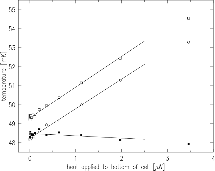
Figure 3-12: Typical measurements used to extract thermal conductance of cell at one temperature. The temperature of the bottom (open symbols) of the cell increases linearly as heat is applied to the bottom. The temperature at the top (solid symbols) stays roughly constant since it is temperature controlled (using a different thermometer as the sensor). The lines are linear fits for the range of powers from 0 to 2.5 $\mu$W. The slopes of the two upper lines give the thermal resistance of the cell at this temperature. The resistances measured by the two thermometers are $1.62\pm 0.04~{}{\rm mK/\mu W}$ and $1.56\pm 0.04~{}{\rm mK/\mu W}$. The 1 mK offset between the two bottom thermometers is due to miscalibration.

Conductances were measured at several cell temperatures. They are compiled in figure 3-13. All temperature rises were less than 10%.

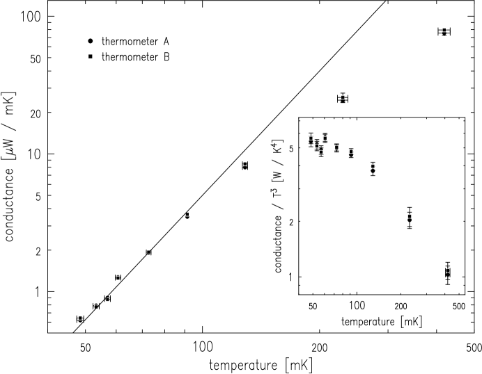
Figure 3-13: Thermal conductance along the length of the cell. The two data sets are from the two thermometers at the bottom of the cell. Approaching low temperatures one expects the conductance to fall like $T^{3}$, as indicated by the line. The inset shows the conductance with this $T^{3}$ dependence factored out. The error bars are the statistical fit uncertainties, and do not include systematics. The vertical error bars in the inset are dominated by the temperature uncertainty. Data without error bars have uncertainties smaller than the symbols.

The conductances measured here are adequate for the experiments we wish to perform.

The thermal conductance across the sinter plates, where heat is transferred from the superfluid to metal and eventually to the refrigerator, may be measured in an analogous way. The temperature of the dissociator was controlled with a thermometer and heater near the top of the dissociator (see figure 3-8). The thermal gradient measured thus includes the thermal resistance across the indium o-ring vacuum seal (superconductivity quenched by 4 T field) and along the length of the dissociator. The data from the two thermometers at the top of the cell were fit to straight lines, similarly to the data in figure 3-12. Two temperatures and conductivities were thus obtained for each temperature control point. These two data sets are shown in figure 3-14.

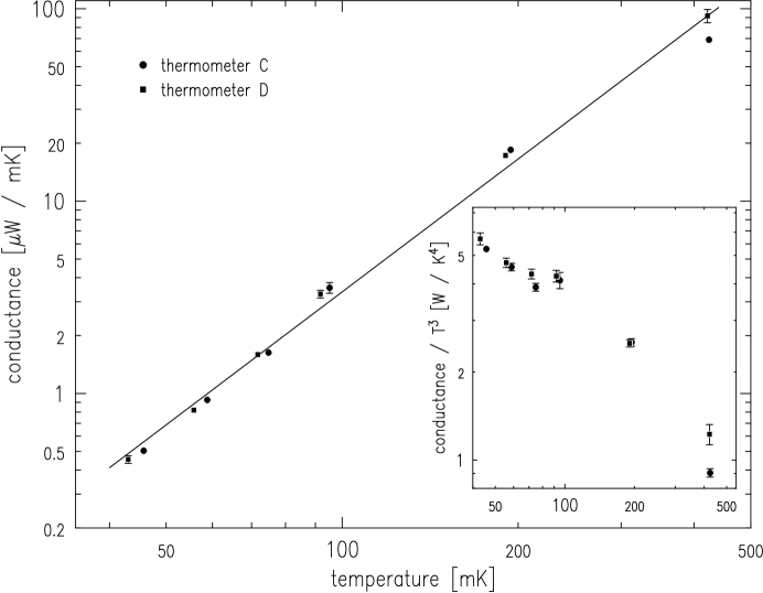
Figure 3-14: Thermal conductance across the Ag sinter, from the superfluid jacket to the metal that comprises the dissociator. The two data sets are from the two thermometers at the top of the cell. Simple acoustic mismatch theory predicts a $T^{3}$ dependence. This is factored out in the inset. The line, a fit to the data points, is $S=(8.6\times 10^{-5}~{}{\rm\mu W/mK^{3.3}})\times T^{2.3}$. The error bars reflect the statistical fit uncertainties. Data without error bars have uncertainties smaller than the symbols.

The conductance of the cell is similar to the conductance across the sinter. Any significant improvements to the thermal conductivity of the system would need to address both of these segments of the heat transport channel.

In a separate experiment the effects of specular and diffuse phonon scattering were studied. A cell similar to that described above was made. The surfaces of the bottom 23 cm of both the inner and outer tubes were sanded with 120 grit paper to create an optically dull finish. The remaining 42 cm exhibited the shiny surface characteristic of the epoxy coating. The thermal conductance of the two sections was measured in the range 50 mK to 300 mK. The section with diffuse optical reflection had a conductance three times lower than the other section. We thus conclude that diffuse reflection reduces the conductivity by a factor of $3\times 42/23\simeq 5$.

3.4.3 Heat Capacity

The heat capacity of the cell and dissociator have been measured together in a typical trap loading sequence. The dissociator was held by a temperature controller at 280 mK for 7 sec while pulsing an rf discharge inside. The heater and discharge where then turned off, and the cell plus dissociator assembly was cooled. The temperature of the bottom of the cell is shown in figure 3-15.

Figure 3-15: Temperature of the bottom of the cell while cooling from 280 mK. The cooling rate is dominated by the heat capacity of other metal parts, not the superfluid.

The cooling rate is expected to be dominated by the large heat capacities of the large copper pieces which comprise the dissociator and mixing chamber. Note that the molar specific heats of copper and ⁴He are nearly identical at 100 mK, and there is much more Cu than ⁴He.

3.4.4 RF Heating

When rf power is introduced into the cryostat the cell and mixing chamber are warmed. Ohmic heating occurs in the coax lines that deliver the power to the cell, and rf eddy currents cause heating of the metals in the vicinity of the coils. Measurements of these heating rates is complicated by imprecise knowledge of where the power is deposited and by disruption of the thermometer readout circuits by the rf fields. Nevertheless, some information can be obtained.

The most reliable piece of information relates to the ejection of atoms from the trap. If the cell becomes too warm, ⁴He atoms evaporate and careen through the trapped sample, knocking atoms out of the trap. In many cases the maximum rf power is set by this criterion. A test was done of this ejection process by simply ramping the rf frequency across the range of interest (23 MHz to 2 MHz) at various rf powers, and noting how many atoms were ejected. To prevent resonant ejection a large bias field was applied so that the minimum resonance frequency of the trapped atoms was always above the applied rf frequency. No ejection was noted for powers up to +27 dBm outside the cryostat (corresponding to about 30 mG fields). The cell thermometers indicated 220 mK (bottom) and 180 mK (top). The maximum rf powers used for the experiments in this thesis were +15 dBm, so ejection of atoms from the trap was not a problem.

Another piece of reliable data is that the cell will stay below 160 mK when rf fields of roughly 5 mG are applied at frequencies of 23 MHz and below. This temperature is low enough to allow the cell to cool reasonably quickly to temperatures at which atoms may be dumped out of the trap and analyzed.

We note that there are a few resonances at which significant heating occurs. These are above 25 MHz. One possible rf leak might occur where the superconducting twisted pair is joined to the coax. Further investigations of where heating occurs should be pursued. Methods could include a consideration of how fast objects cool when the rf is turned off and the time required for heat to reach various thermometers.

Chapter 4 Manipulating Cold Hydrogen by RF Resonance

Resonant RF ejection of atoms from the trap is a tool for manipulating and studying the hydrogen gas. This tool has not previously been applied to trapped hydrogen, and so the peculiarities of this system have not been explored. We find—as anticipated—that rf ejection can efficiently remove energetic atoms that would otherwise not find their way out of the trap over the magnetic saddlepoint barrier. Experiments are described in section 4.1. Furthermore, we find that rf ejection spectroscopy can constitute a valuable diagnostic technique near BEC, where the trap dump technique used previously fails. RF ejection spectroscopy is also an essential tool for measuring the magnetic field at the bottom of the trapping potential. These topics are covered in section 4.2.

4.1 RF Evaporation

4.1.1 Need for RF Evaporation: Orbits with Long Escape Times

In section 2.1 we explained that, for low temperature samples in tightly compressed traps, the saddlepoint evaporation technique leads to one dimensional evaporation. Recall that atoms with high radial energy are unable to escape before having a collision. In this section we demonstrate this problem experimentally.

Three successive samples are identically prepared by cooling into a trap with depth $\epsilon_{t}/{k_{B}}=1.1$ mK, set by a magnetic saddlepoint. The trap radial gradient is $\alpha/{k_{B}}=4.4$ mK/cm. After the evaporation cycle is completed, the sample is held for many seconds ($\sim 20$), on the order of three characteristic collision times. The saddlepoint barrier is then reduced to zero in 5 s while the atom flux is recorded as a function of barrier height by sensing the heat of molecular recombination on a sensitive bolometer (section 4.2.3). In its simplest interpretation, this flux profile is the energy distribution of the trapped cloud. (Corrections to this picture will be described in section 4.2.1). Figure 4-1 shows atom flux profiles for the three samples.

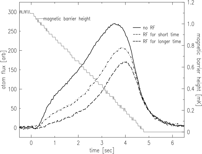
Figure 4-1: Comparison of dump signals from samples with and without rf ejection. The solid sloping line shows the trap depth as it is reduced from 1.1 mK to zero. The curves indicate the atom flux as the trap depth is reduced. The dashed curves correspond to a samples that were exposed to rf tuned to the trap depth for 9 s and 23 s. The solid curve corresponds to a sample with no rf exposure. The rf fields eject a sizeable fraction of the sample and change the shape of the profile. The response time of the detection process is seen at the end of the ramp, at t=5 s.

The largest profile is for a sample (sample 1) that was held for 10 s, and then dumped from the trap. For the smaller two profiles, a weak rf field resonant at the trap depth (${\epsilon_{t}}=h\nu_{rf}-\theta$) was applied for 9 s (sample 2) and 23 s (sample 3) at the point in the sequence where sample 1 was held. The samples were then dumped out of the trap in the same way as sample 1. We see that a significant fraction of the atoms have been ejected from samples 2 and 3. To be ejected, these atoms must have had a total energy that was above the magnetic saddlepoint energy. Since these atoms did not leave the trap in sample 1, they were apparently in orbits with escape times of at least ten seconds. This experiment demonstrates the long times required for energetic atoms to escape when the energy barrier is set only by a magnetic field saddlepoint at one end of the trap, and the reduction in escape time when the atoms can leave in any direction. Furthermore, the decrease in trap population between samples 2 and 3 indicates the long thermalization time of the system as it equilibrates to the lower effective trap depth for the radial degrees of freedom. This trap had a radial confinement that was a factor of $\sim 3$ weaker than those used for attaining BEC as described in section 5.2, and so these experiments place a lower bound on the problem.

4.1.2 Mixing of Energy

It is postulated that there is only very weak coupling among the motional degrees of freedom of a particle moving in the trap potential. This weak coupling between transverse and axial degrees of freedom is the impetus for driving evaporation with rf fields. In this section we describe a simple experiment which demonstrates this very weak coupling.

Four identically prepared samples are each cooled into a trap with depth ${\epsilon_{t}}=1.1$ mK and radial gradient $\alpha=4.5$ mK/cm. The trap is significantly longer than the one shown in figure 3-4, with the sample extending from roughly $z=-6$ cm to $z=+9$ cm. The sample is adiabatically expanded by opening the trap slowly, reducing the radial gradient to $\alpha=1.3$ mK/cm, but leaving the length constant. The peak sample density is approximately $n_{0}=4\times 10^{12}~{}{\rm cm^{-3}}$. The thermalization time is thus on the order of 10 s, and the dipolar decay time is on the order of $10^{3}$ s.

Figure 4-2 shows the flux of atoms escaping the trap as the magnetic confinement field at one end of the trap is linearly ramped to zero.

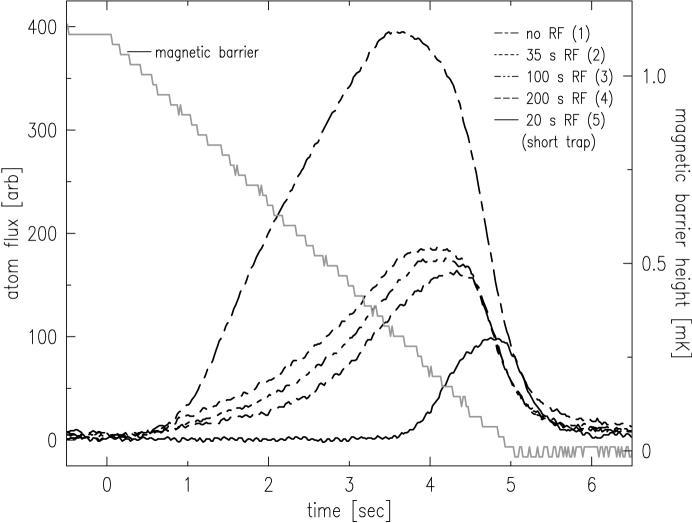
Figure 4-2: Demonstration of slow transfer of energy from axial to transverse motional degrees of freedom. The five curves are the flux of atoms escaping the trap as the magnetic energy barrier at one end of the trap is slowly ramped to zero (linearly sloping line), for each of five samples. The samples labeled 1-4 correspond to various durations of exposure of the sample to 10 MHz rf fields with strengths of a few milligauss. Sample 5 was confined in a short trap, and was exposed to an rf field at 10 MHz for 20 s. The field had ten times more power than for samples 1-4.

As explained above, this atom flux can be interpreted as an indication of the distribution of energies of the trapped atoms. The four traces labeled 1-4 correspond to the four samples. The first sample was simply held in the trap for 20 s after preparation, and then dumped. The second, third, and fourth samples had an rf field (a few milligauss strength) applied for various times—35 s, 100 s, and 200 s. The frequency (10 MHz) corresponds to slightly less than half the trap depth set by the magnetic field barrier at the end of the trap. Even though the rf field is produced by both the axial and transverse coils, the rf fields have significant strength (and appropriate polarity) only along the sides of the trap, and not at the ends. We expect the rf fields to only eject atoms with energy in the transverse (not axial) directions.

Comparing sample 1 to sample 2, we see that about two-thirds of the atoms are ejected when the rf is applied for 35 s, and that the energy distribution is narrowed, a sign of cooling. As the rf exposure is continued (samples 3 and 4), a few more atoms are ejected, and the sample continues to slowly cool. Two time scales thus appear. The fast time scale ($\sim 10$ s) must correspond to removal of atoms with high energy in the transverse degrees of freedom. These atoms interact directly with the rf fields. The slow time scale ($\sim 100$ s) is for removal of atoms that originally had high energy in the axial degree of freedom, but low energy in the transverse direction. It apparently takes on the order of 100 s for enough energy to transfer from axial motion to transverse motion to allow the atoms to reach the resonance region.

This interpretation is supported by the data shown in figure 4-2 for sample 5. This sample was prepared identically to samples 1-4, but the trap was short. There was significant field strength (and appropriate polarity) at the ends as well as the sides of the trap, so that atoms with high energy in either the axial or the transverse direction could pass through the resonance region (again, both transverse and axial coils are used, as is done for the routine rf evaporation in chapter 5). The resonance region wraps completely around the sample, in contrast to samples 1-4 for which the resonance region is essentially a tube around half the length of the sample. We observe that the energy distribution is narrowed very significantly with only short application of the rf field. This happens because energy does not need to mix among degrees of freedom before ejection can occur.

4.1.3 RF Field Strength Required for Evaporation

As discussed in section 3.1.3, the rf field strength used during evaporation must be strong enough to eject energetic atoms from the trap before they have a collision. We have experimentally determined this power requirement for a typical sample density and trap shape. A series of samples are identically prepared at $T\sim 70~{}\mu$K, and then evaporatively cooled to a given trap depth using rf fields of varying power. After this rf cooling cycle the atoms are dumped from the trap, and the total number of trapped atoms is recorded. For very low rf powers essentially no rf evaporation occurs, and the sample is not depleted. For higher powers the sample is significantly depleted, up to an rf power that saturates the process. At this high power, energetic atoms are promptly removed before having a collision; no further sample depletion is possible with increasing power because the atom ejection rate is no longer bottlenecked by the rf ejection rate, but rather by the rate at which collisions in the gas create energetic atoms.

Figure 4-3 shows one such saturation measurement.

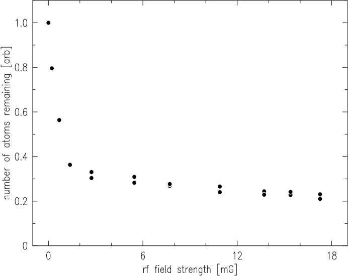
Figure 4-3: Determination of the field strength required for rf evaporation. Atoms are depleted from the sample by fields of various strengths during an rf evaporation cycle. The peak sample density is $n_{0}\sim 7\times 10^{13}~{}{\rm cm}^{-3}$ and the trap radial gradient is $\alpha/{k_{B}}=4.5$ mK/cm. The horizontal scale is the peak rf field strength, as estimated from room temperature measurements. There is a factor of two scale uncertainty which arises from imprecise knowledge of the temperature dependence of the impedances and of the details of the field geometry.

The rf frequency is swept from 17 MHz to 9.7 MHz at various rf field strengths. Two thirds of the atoms are removed when the field strength is above 2 mG. This agrees well with the calculation in section 3.1.3. Note, however, the large scale uncertainty on the horizontal axis. Ideally we would plot an effective field strength which is the appropriate average of the ejection rate over the resonance surface (see section 4.2.2); ignorance of the details of the rf field direction and strength makes this average difficult. We have therefore plotted on the horizontal axis the strength of the field at low frequencies, as measured at one point in the cell at room temperature for a given power applied outside the cryostat. A correction was made for the frequency response measured in section 4.2.5, assuming a driving frequency of 10 MHz. The number of remaining atoms continues to slowly drop as a function of field strength even for fields much greater than the saturation field of 2 mG. This behavior is not understood. It might indicate the presence of atoms in high angular momentum orbits which only very rarely cross the resonance region.

4.2 RF Ejection Spectroscopy

The simple technique of rf ejection spectroscopy is useful as a diagnostic of the temperature and density of the trapped gas near BEC. It has significant advantages over the trap dump technique used previously, which becomes completely ambiguous near the BEC threshold. For probing the condensate, the technique is inferior to optical spectroscopy (described in section 5.1.1), but it is much simpler to use. In this section we explain the problems which make the trap dump technique ambiguous. We then develop a theory that explains the rf ejection measurements. After an explanation of the bolometric detection process employed in the rf ejection spectroscopy, we show how the technique can be used to measure the magnetic field at the bottom of the trap and to measure the temperature of a cold sample.

4.2.1 Ambiguities of the Trap Dump Technique

In previous experiments the sample was studied by dumping it from the trap and measuring its energy distribution (see section 2.5 and 2.6 in [17]); the distribution was inferred by measuring the flux of escaping atoms as the axial trap barrier was reduced (see figure 4-1 for example). Ambiguities arise, however, because of conflicting timescales. In order to measure an energy distribution, the flux detector must respond in a time $\tau_{det}$ which is short compared to the duration over which the trap energy threshold is reduced to zero, $\tau_{dump}$. Furthermore, the characteristic sample equilibration time, $\tau_{equil}$, must be long compared to $\tau_{dump}$ so that the energy distribution does not change during the dump process. For the dense samples studied near the BEC transition the equilibration time is $\tau_{equil}\sim 300$ ms. The detector response time is $\tau_{det}\sim 200$ ms. A further crippling complication is that the characteristic escape time, $\tau_{esc}$, for an atom with total energy greater than the trap depth must be short compared to $\tau_{dump}$ so that all of the atoms in a given energy slice leave the trap before atoms from the next slice begin to come out; in the tightly compressed traps used near the BEC transition this escape time has been observed to be many tens of seconds, as demonstrated by figure 4-1. The timescale hierarchy,

$$\tau_{det},\tau_{esc}\ll\tau_{dump}\ll\tau_{equil}$$ (4.1)

is not achievable, and the trap dump technique fails to providing reliable measurements of the energy distribution of samples near the BEC regime. There is also a practical problem. As the axial confinement magnetic field is lowered, the trap shape changes. Often a magnetic field zero forms, further complicating the measurements.

RF ejection spectroscopy, in which a resonance region is tuned through the trap to eject atoms with various potential energies, addresses all these problems. The trap shape remains unchanged, so no zeros are introduced. The particle escape time can be short because atoms are coupled out in all directions. Finally, the energy distribution of the sample does not change significantly during the measurement process because only a small fraction of the atoms are removed.

4.2.2 Theory of RF Ejection Spectroscopy of a Trapped Gas

In this section we use the results of the Landau-Zener theory discussed in section 3.1.2 to explain the rf ejection spectrum expected for a trapped gas, i.e. the flux of atoms ejected as a function of the frequency of the rf magnetic field. This expression is used to interpret the spectra presented later in the chapter.

Consider a sample trapped in a magnetic potential $V({\bf r})=\mu_{B}\left|{\bf B}_{trap}({\bf r})\right|$ described by the potential energy density of states function $\varrho(\varepsilon)$. The bottom of the trap is at a magnetic field $B_{0}=\theta/\mu_{B}$. An rf magnetic field, oscillating at frequency $\nu_{rf}$ with strength ${\bf B}_{rf}$, is superimposed on the trap, and resonantly interacts with atoms crossing a surface of constant potential $\varepsilon_{res}=h\nu_{rf}-\theta$. For the analysis that follows we note that this surface area and its differential thickness is related to $\varrho(\varepsilon)\;d\varepsilon$, which is the differential volume in the trap with potential energy in a range $d\varepsilon$ around $\varepsilon$. This volume may be written as an integral, over the area of the surface of constant $\varepsilon$, of the differential “thickness” $d\varepsilon/|\alpha({\bf r})|$ of the surface:

$$\varrho(\varepsilon)\;d\varepsilon=\int dA\frac{d\varepsilon}{|\alpha({\bf r})|}$$ (4.2)

where $\alpha({\bf r})$ is the gradient of the potential at position ${\bf r}$. This result will be used to derive equation 4.6.

We wish to find the rate at which atoms leave the trap as a result of Zeeman sublevel transitions in the resonance region. In a patch of resonance surface of differential area $dA$ at position ${\bf r}$, the differential atom loss rate is $d\dot{N}=FP\;dA$, where $F$ is the flux passing through the surface from either direction and $P$ is the probability of the atom emerging from the resonance surface in an untrapped Zeeman sublevel. Equations 3.23 and 3.24 indicate that, in the limit of low rf field strength, the vast majority of transitions are made from the $d$ to $c$ Zeeman sublevels. The transition probability is $P=P_{c}=2(1-p)p$, where $p=1-\exp(-\zeta)$ and $\zeta({\bf r},v)=\pi\mu_{B}^{2}B_{rf}^{2}({\bf r})/\alpha({\bf r})v\hbar$ is the adiabaticity parameter for an atom with velocity $v$ passing through resonance at a position ${\bf r}$. Here $B_{rf}$ is the component of the rf field that is perpendicular to the dc trapping field. In the weak field approximation, $P\simeq 2p$ and $p\simeq\zeta$. The transition probability exhibits a velocity dependence. The flux of atoms with velocity $v$ passing through the surface is $F(v)=n({\bf r})f_{v}(v)v$ where $f_{v}(v)$ is a normalized one dimensional velocity distribution function, such as derived in appendix E, and $n({\bf r})$ is the density at position ${\bf r}$ (either the Bose-Einstein or Maxwell-Boltzmann density, as appropriate). Since both $P$ and $F$ exhibit a velocity dependence, the differential atom loss rate must be derived from an integral over velocities

$$d\dot{N} = dA\int dv\;n({\bf r})f(v)v\>2\zeta({\bf r},v)$$ (4.3)

$$= dA\;\frac{2\pi\mu_{B}^{2}B_{rf}^{2}({\bf r})n({\bf r})}{|\alpha({\bf r})|\hbar}.$$

The total atom loss rate ${\cal F}(\varepsilon)$, through a resonance surface at potential energy $\varepsilon$, is

$${\cal F}(\varepsilon) = \int d\dot{N}$$ (4.4)

$$= \frac{2\pi\mu_{B}^{2}n(\varepsilon)}{\hbar}\;\int dA\frac{B_{rf}^{2}({\bf r})}{|\alpha({\bf r})|}$$

$$= \frac{2\pi\mu_{B}^{2}}{\hbar}\;n(\varepsilon)\>B_{eff}^{2}(\varepsilon)\varrho(\varepsilon).$$ (4.5)

Here we have defined $B_{eff}$ as an effective rf field strength obtained by a weighted average, over the resonance surface, of the magnitude of the component of the rf field that is orthogonal to the trapping field, ${\bf B}_{trap}$. The weight function is the thickness of the surface. Using equation 4.2

$$B_{eff}(\varepsilon)\equiv\left(\frac{1}{\varrho(\varepsilon)}\int_{V({\bf r})=\varepsilon}dA\;\frac{\left({\bf B}_{rf}({\bf r})\times{\bf B}_{trap}({\bf r})\right)^{2}}{|\alpha({\bf r})|B_{trap}^{2}({\bf r})}\right)^{1/2}.$$ (4.6)

If the polarization of ${\bf B}_{rf}$ is randomized all over the resonance surface, then the cross product in equation 4.6 is essentially a scalar product, and $B_{eff}(\varepsilon)$ is the average, over the equipotential surface, of the square of the rf field strength. This approximation is similar to a random phase approximation. Furthermore, if the length scale for variations in the field strength is significantly different from the size of the trap, then the field averaged over the surface will be independent of the equipotential chosen. Certainly if the field is uniform over the trap (characteristic length long compared to size of trap), then the average of the field over the equipotential surface does not depend on which surface is chosen. In the other limit, if the characteristic length scale of the fluctuations in the field strength is short compared to the size of the trap, then the variations average out over the surface regardless of the surface chosen. The result in either case is that $B_{eff}$ is independent of $\varepsilon$. The field generated in the cell by a given rf driving power, measured outside the cryostat, can vary as a function of frequency; this “transfer function” is an artifact of the reactance of the coils and the drive line impedance, and is measured in section 4.2.5. This dependence is not included here.

In our experiment these two approximations (random orientation and incommensurate length scale) are not so bad; the rf field is a superposition of the fields generated by both the transverse and axial coils. The strength of the axial field varies on a length scale much shorter than the trap length, but much longer than the trap diameter, due to the field compensation scheme employed. Figure 3-4 shows the strength of the axial field along the symmetry axis of the trap. The field of the transverse coil is essentially uniform all across the trap. Since the relative strengths of the rf field components vary all over the trap, the direction of the field also varies. Tests of this simplifying assumption are outlined in section 4.2.5. The relative phase of the axial and transverse field is assumed to be zero, independent of frequency and position. Violations of this assumption have not been considered.

If $B_{eff}$ has no strong dependence on $\varepsilon$, then the flux of atoms ejected from the trap for a given $\nu_{rf}$ is proportional to the number of atoms with potential energy $\varepsilon$, $n(\varepsilon)\varrho(\varepsilon)$, as found in equation 4.6. A distribution of potential energies may thus be obtained by sweeping the resonance surface through the trap. This distribution can be used to infer the sample temperature.

In the derivation of equation 4.3, we made the approximation that the rf power was low. We assumed that $\zeta\ll 1$. Inverting equation 3.1.2, this requires that $B_{rf}\ll\sqrt{\alpha v\hbar/\pi\mu_{B}^{2}}$. For typical parameters $mv^{2}/2=(50~{}\mu{\rm K}){k_{B}}/10$ and $\alpha/{k_{B}}=(16~{}$mK/cm) the requirement is that $B_{rf}\ll\sim 20$ mG. Near the bottom of the trap where the potential flattens the small gradient implies that the experimenter must use very low rf field strength to remain in the low rf power regime.

A further approximation used in the interpretation of the spectra is that the sample’s energy distribution does not change while the spectrum is being measured. This condition could be fulfilled by measuring the spectrum quickly compared to the rethermalization time, but, as explained above, the response time of the detection process is too slow. Another way to realize this condition is to remove only a small fraction of the atoms while obtaining the spectrum. The number of atoms ejected from the trap in a duration $\tau_{spec}$ is $N_{eject}=\int_{0}^{\tau_{spec}}dt\;{\cal F}(\varepsilon(t))$. For a linear ramp of the resonance from the bottom to the top of the trap, we have $\varepsilon(t)=(\varepsilon_{t}/\tau_{spec})t$ and

$$N_{eject} = \frac{2\pi\mu_{B}^{2}B_{eff}^{2}\tau_{spec}}{\hbar\varepsilon_{t}}\;\int_{0}^{\varepsilon_{t}}n(\varepsilon)\>\varrho(\varepsilon)\>d\varepsilon$$ (4.7)

$$= \frac{2\pi\mu_{B}^{2}B_{eff}^{2}\tau_{spec}}{\hbar\varepsilon_{t}}\;N$$

where $N$ is the trap population. A spectrum should be obtained over a duration, $\tau_{spec}$, much longer than the detector response time; in practice we use $\tau_{spec}\sim 5$ s. For a trap depth of 1 mK we obtain the condition $B_{eff}\ll\sqrt{\hbar\varepsilon_{t}/2\pi\tau_{spec}}/\mu_{B}\sim 200~{}\mu$G. This low ejection rate condition can be difficult to fulfill while simultaneously enjoying a large signal-to-noise ratio in the detector.

4.2.3 Bolometric Detection

Atoms coupled out of the trap by rf resonance are detected by sensing a small fraction of the molecular recombination heat they liberate. The detection process is explained in detail by Doyle [17]. Atoms (in the $c$-state) leaving the trap stick to the cell wall. A fraction experience a spin flip to the $b$- or $a$-state, opening the way for rapid recombination. If the residence time on the wall is long enough, and if the time associated with sliding along the wall out of the detection region and into a high field region is long enough, and if the surface density is high enough, then the vast majority of the atoms will recombine. The heat deposited on the bolometer will be proportional to the number of atoms which escaped from the trap. The picture is modified slightly for the rf spectroscopic studies presented here because the atoms are ejected in the $c$-state instead of the doubly spin-polarized $d$-state treated by Doyle. State mixing should occur rapidly, however, induced by magnetic impurities on the walls, and so the remaining considerations are still valid. They indicate that the cell walls should be cold (80 mK) and that the atom flux should be high. Both of these conditions impose limitations on the techniques described here. We observe well resolved rf spectra with atom fluxes on the order of $10^{9}$ atoms per second falling out of the trap toward the bolometer.

Crucial to the interpretation of the spectra presented is an understanding of the time response of the bolometric detection process, as suggested above. The impulse response function of the detection system was measured directly using a series of 200 ms rf pulses at various frequencies for samples of two different temperatures in the range of interest. Figure 4-4 shows a typical pulse

Figure 4-4: Impulse response of detection system. An rf pulse is applied for 200 ms, and the resulting bolometer signal is recorded. For this pulse the fit delay time is $\tau_{delay}=277$ ms, the fall time is $\tau_{fall}=340$ ms, and the effective rise time is $\tau_{rise}=251$ ms. The heat in this pulse is 2.6 pJ, which corresponds to the heat from $3\times 10^{6}$ recombination events. The quiescent power applied to the bolometer was 100 pW, the bolometer temperature was 180 mK, and the cell temperature was 90 mK.

and an analytic fit of the form

$$g(t^{\prime})=\left\{\begin{array}[]{ll}\frac{g_{0}}{\tau_{fall}-\tau_{rise}}\left(e^{-t^{\prime}/\tau_{fall}}-e^{-t^{\prime}/\tau_{rise}}\right)&t^{\prime}\geq 0\\ 0&t^{\prime}<0\end{array}\right.$$ (4.8)

where $t^{\prime}=t-\tau_{delay}$. This form was chosen to model the time constants for an atom to stick to the wall and to find a recombination partner. The fit parameters were consistent to about 10% for all the pulses, and the average values were $\tau_{delay}=299$ ms, $\tau_{rise}=246$ ms, and $\tau_{fall}=337$ ms. The dependence of these parameters on the film thickness has not been studied systematically, but at low film thicknesses the H-He binding energy increases and the atoms stick promptly; $\tau_{delay}$ decreases. Because the rf pulse has finite duration, the measured response is not, strictly speaking, the impulse response function. Nevertheless, it is a good approximation, and the analytic fit parameters quoted above were used in calculating the spectra presented in the following sections.

The response time of the bolometer readout electronics was measured by heating the bolometer with short pulses of light from a HeNe laser. The response time was approximately $10^{-3}$ s, negligible compared to the time constants for recombination.

4.2.4 Measuring the Trap Bias Field

The bias field in the Ioffe-Pritchard trap, $\theta/\mu_{B}$, sets the characteristic sample temperature at which the trap functional form changes from predominantly linear ($T\gg\theta/{k_{B}}$) to predominantly harmonic ($T\ll\theta/{k_{B}}$) in the two radial dimensions. It is thus an important quantity for analysis of Bose condensation experiments. Furthermore, to know the trap depth $\epsilon_{t}=h\nu_{rf}-\theta$, one must know both the trap energy barrier (set by the experimenter) and the bias energy.

The bias is directly measured by sweeping up the frequency of the rf field until atoms begin to be ejected from the trap. Figure 4-5 shows such a sweep.

Figure 4-5: Measurement of trap bias using rf ejection. The rf field is switched on at $t=0$ and swept from 200 kHz to 1.2 MHz. The atoms begin to leave the trap at about 700 kHz. The sloping baseline signal results from atoms evaporating out of the trap as the sample continues to cool after the end of the forced evaporative cooling cycle.

The atoms begin to be coupled out of the trap at about $t=5$ s, corresponding to a frequency $\nu_{\theta}=700$ kHz; in this case we find $\theta/{k_{B}}=\nu_{\theta}h/{k_{B}}=33.6~{}\mu$K. RF ejection is a powerful and sensitive technique to quickly and accurately measure the absolute trap bias.

The bias can also be inferred by deforming the trap potential until a field zero is created; atoms begin to experience Majorana flips, leave the bottom of the trap, and get detected by the bolometer. The zero is made by changing the current in a solenoid that creates a fairly uniform field along the length of the trap. Integration of the Biot-Savart law gives the field strength per unit current. This method of finding the bias field is not as accurate as the rf ejection method since the trap shape is deformed for the measurement. Nevertheless, the two methods agree to within the experimental uncertainties.

4.2.5 Measuring the Effective RF Field Strength

In order to analyze rf ejection spectra, one must know the effective rf field strength, $B_{eff}$ given by equation 4.6. It may exhibit complicated polarization dependences if the random orientation and incommensurate length scale approximations made in the discussion of equation 4.6 are invalid. Furthermore, there may be a frequency dependence in the field strength generated in the cell by a given rf power applied outside the cryostat, as discussed in section 3.4.1. Clearly a measurement of the efficiency is in order.

RF spectra were measured to verify the ejection efficiency for frequencies between 1 and 17 MHz. The ejection rate at a given frequency, given by equation 4.5, includes the density, the potential energy density of states, and the effective rf field strength. In order to simplify the measurement of the efficiency, the density was kept constant over the energy range of interest by using a warm sample, $T\sim 1$ mK$>h\nu_{max}/{k_{B}}$. The potential energy density of states functional form is known well. The quantity obtained, then, is the ejection efficiency as a function of frequency. The flux ejected as the frequency of the rf field was swept upward is shown in figure 4-6 for the axial coil alone, the transverse coil alone, and both coils together.

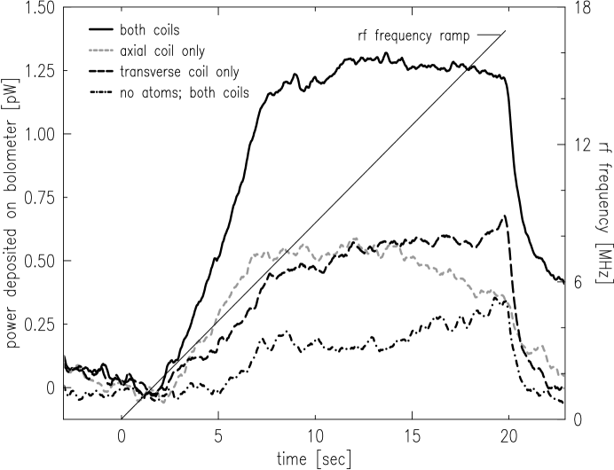
Figure 4-6: Ejected atom flux as the rf frequency is swept through the trap. The lowest sweep indicates the rf pickup and heating loads; no atoms were in the trap and both coils were driven. For the middle two sweeps only a single coil was driven. For the top sweep both coils were driven. The point at which atoms start to leave the trap, $t\sim 2$ s, indicates the bias field. Atoms stop leaving the trap when the rf field is extinguished, $t\sim 20$ s. At the lower frequencies the rf field strength is $\sim 3\times 10^{-4}$ G. Apparently the transverse coil is responsible for most of the heating at high frequencies.

Another sweep, taken with no atoms in the trap but with both coils driven, indicates rf pickup and heating effects.

The simplest model of the frequency dependence of the ejection efficiency ignores polarization effects and accounts only for impedance matching (the voltage divider effects of the reactance of the coils and the 50 $\Omega$ feed lines); we take

$$B_{eff}(\omega)\propto\left|\frac{1}{1+i\omega/\omega_{0}}\right|$$ (4.9)

Figure 4-7 indicates the expected spectra for three values of $\omega_{0}$.

Figure 4-7: Determination of the frequency response of the coils by a comparison of calculated and measured spectra. The measured spectrum has the background, shown in figure 4-6, subtracted. The only adjustable parameters in the calculated spectra are the overall normalization, the baseline, and $\omega_{0}$.

Evidently $\omega_{0}\simeq 2\pi\times 8$ MHz, which agrees reasonably with the measured response of the coils below 20 MHz at room temperature (figure 3-11). This value is used in the calculated spectra presented next.

4.2.6 Determining the Sample Temperature by RF Ejection Spectroscopy

As suggested in equation 4.5, rf ejection spectroscopy can give the temperature of the sample since it gives the potential energy distribution of the trapped atoms. This spectrum is different from the total energy distribution obtained by dumping the atoms out of the trap, as done in previous hydrogen experiments [23, 17], or by saturating the rf transition for the entire sample [81, 82]. The difference between the total and potential energy distributions is indicated in figure 4-8.

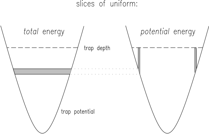
Figure 4-8: Probing the distribution of total energy and potential energy of a trapped sample. The total (potential) energy distribution function gives the number of particles with a given total (potential) energy. The shaded area is the region of atoms probed by the technique. The solid lines indicate the trapping potential, and the dashed line is the trap depth.

As outlined above, the rf ejection spectroscopy technique is free of several complications implicit in the trap dump technique. RF ejection spectroscopy has been employed to measure the temperature of the coldest samples of trapped H to date, a factor of 40 colder than the photon recoil cooling limit.

Figure 4-9 shows the spectrum of a sample that was cooled to $T=30~{}\mu$K by rf evaporation.

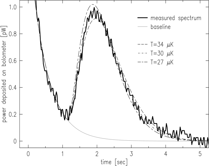
Figure 4-9: RF spectrum of trapped gas at $30~{}\mu$K. The heavy line is the raw data. The thin solid line is the inferred background, whose functional form has been verified independently. The three dashed lines are calculations of the spectrum for different temperatures assuming quantum degeneracy. The calculations include the time response of the detection system, the measured trap depth, and the measured effective rf field strength. The only remaining adjustable parameter is the normalization. The rf field strength used for this spectrum is $\sim 200~{}\mu$G.

This sample should contain a small condensate, although it is not visible here. The three calculated spectra in figure 4-9 assume quantum degeneracy. Furthermore, they include the measured time response of the detection system, the measured trap bias, and the measured effective rf field strength. Possible distortions, not considered in the calculations, arise from sample depletion during the rf sweep and changing detection sensitivity due to nonlinearities in the detection process at low atom fluxes. This second effect should be small, as suggested by the quality of the calculated rf ejection spectrum, which ignored nonlinearity. The first effect can be shown to be small by taking a series of such spectra at various rf powers, thus depleting the sample by various (small) amounts. Of course at lower powers the signal/noise ratio becomes smaller; the power used for the spectrum in figure 4-9 involves a compromise between signal size and distortion. The apparent temperature is shifted no more than 10%.

Determination of sample temperature through rf ejection spectroscopy is limited by the signal rate, which is proportional to $N_{eject}/\tau_{spec}$ in equation 4.7. The technique could be extended to much lower temperatures if the detection efficiency is improved.

A practical limitation involves the requirement that the cell walls be cold enough to support a long atom residence time, and thus high recombination efficiency. Because of rf heating effects, this limitation usually requires the rf power to be reduced for several seconds before the rf spectrum is obtained. The sample can warm during this time since the trap depth is not as well defined.

Chapter 5 Observation of BEC

In this chapter we describe the first observations of Bose-Einstein condensation of hydrogen.

Our primary diagnostic technique is laser spectroscopy, which we briefly describe here; detailed descriptions are given by Sandberg [16] and Killian [13] (Killian’s thesis should be considered a companion to this chapter). With this probe we are able to monitor the density and temperature of the gas as the temperature is reduced by rf evaporation. When the gas is cooled into the quantum degenerate regime signatures of the Bose-Einstein condensate appear in the spectrum; these can be analyzed to reveal the size and population of the condensate. As anticipated, the condensate is huge, containing a factor of 50 more atoms than condensates in other experiments, and having a length on the order of a centimeter. We are able to study the time evolution of the condensate, which is governed by feeding of the condensate from the thermal gas. We explore some of the implications of these results for the production of high-flux coherent atomic beams.

5.1 Laser Spectroscopy of Trapped Hydrogen

Laser spectroscopy of trapped atomic hydrogen has been pursued as both a technique to study and manipulate a trapped gas, and as a probe of the collection of individual atoms for metrology and fundamental measurements [24, 16, 14, 83]. We focus here on spectroscopy as a tool to measure the density and temperature of the trapped gas. It has been suggested that the coherence properties of Bose-condensed atoms could be exploited to perform much improved fundamental measurements [84, 85].

The principal transition in hydrogen, $1S$-$2P$, has a large transition rate, but is difficult to use for sample diagnostics because it has a large linewidth (100 MHz), it suffers from complicated magnetic structure, and it is in the uv (121.6 nm). The transition has been used by the Amsterdam hydrogen trapping group as a diagnostic for warm samples, and also for limited laser cooling and laser induced evaporation [86, 87, 88]. The Doppler effect can be used to measure the sample temperature, but the short $2P$ lifetime limits the technique to temperatures above a few mK. In order to circumvent the short $2P$ lifetime, the Amsterdam group employed two-photon spectroscopy to the $3S$ (160 ns) and $3D$ (16 ns) states [89]. To enhance the two-photon transition rate, one photon was tuned near the Lyman-$\alpha$ resonance and the other near the Balmer-$\alpha$. In principle the $1S$-$3S$ transition could be used for temperature measurement all the way into the sub-$\mu$K regime.

5.1.1 Spectroscopy of the $1S$-$2S$ Transition

We employ the $1S$-$2S$ transition and drive it with two photons at 243 nm, twice the Lyman-$\alpha$ wavelength. The $2S$ state is metastable with lifetime $\tau_{0}=120$ ms, and the natural linewidth is below 1 Hz. The transition thus constitutes a very sensitive probe, through shifts and broadenings, of the local environment of the atom. As explained below, the transition can be used to measure the density of the gas, in addition to the temperature.

To excite the transition the laser beam is retroreflected to create a standing wave in the atom cloud. In this configuration the atom may absorb two photons from the same beam or one photon from each beam. Absorption of co-propagating photons involves the Doppler shift, and the excitation is said to be “Doppler-sensitive” (DS). In the absorption of counter-propagating photons the Doppler effect cancels to first order, and the process is termed “Doppler-free” (DF).

The energy equation for two-photon excitation of an isolated atom from state $i$ to $f$, with initial momentum ${\bf p}_{i}$ and final momentum ${\bf p}_{f}={\bf p}_{i}+\hbar({\bf k}_{1}+{\bf k}_{2})$, where ${\bf k}_{1}$ and ${\bf k}_{2}$ are the wave vectors of the laser beams, is

$$2h\nu=\sqrt{p_{f}^{2}c^{2}+(mc^{2}+2h\nu_{o})^{2}}-\sqrt{p_{i}^{2}c^{2}+(mc^{2})^{2}}.$$ (5.1)

where the rest mass of the atom in the initial state is $m$ and $2\nu_{o}=2.466\times 10^{15}$ Hz [90] is the unperturbed transition frequency. Expanding, we obtain

$$\nu=\nu_{o}+\underbrace{\frac{({\bf k}_{1}+{\bf k}_{2})\cdot{\bf p}_{i}}{4\pi m}\left(1-\epsilon\right)}_{\textstyle\Delta\nu_{D1}}+\underbrace{\frac{\hbar({\bf k}_{1}+{\bf k}_{2})^{2}}{8\pi m}\left(1-\epsilon\right)}_{\textstyle\Delta\nu_{R}}-\underbrace{\frac{\nu_{o}p_{i}^{2}}{2(mc)^{2}}}_{\textstyle\Delta\nu_{D2}}+O(\epsilon^{3}).$$ (5.2)

Here $\Delta\nu_{D1}$ and $\Delta\nu_{D2}$ are the first and second order Doppler shifts, respectively, $\Delta\nu_{R}$ is the recoil shift, and $\epsilon=2h\nu_{o}/mc^{2}=1.1\times 10^{-8}$ is a relativistic correction which accounts for the mass change of the atom upon absorbing energy $2h\nu_{o}$. For hydrogen in the submillikelvin regime, $\Delta\nu_{D2}\ll 1$ Hz and can be neglected. In the Doppler-sensitive configuration, ${\bf k}_{1}={\bf k}_{2}$ and $\Delta\nu_{R}=6.7$ MHz. (All frequencies are referenced to the 243 nm laser source). At a temperature of $50~{}\mu$K, $\Delta\nu_{D1}\sim 2.6$ MHz, and thus the Doppler-sensitive peak is well separated from the Doppler-free. In the Doppler-free configuration, ${\bf k}_{1}=-{\bf k}_{2}$, and there is no recoil or first order Doppler broadening. A spectrum is shown in figure 5-1.

A complete discussion of the shape of the Doppler-free line in the various regimes of density and temperature is presented in the thesis of Thomas Killian [13]. We summarize his discussion by noting that the narrow intrinsic linewidth allows the spectrum to be used for measuring the density and temperature of the sample. The density is measured through the cold collision frequency shift, the low temperature analog to the more familiar pressure shift. In the presence of a cloud of atoms of density $n$ in the $1S$ electronic state, an atom in state $\sigma$ experiences a shift of its energy by an amount $8\pi\hbar^{2}a_{\sigma-1S}n/m$, where $m$ is the atomic mass and $a_{\sigma-1S}$ is the $s$-wave scattering length which parameterizes collisions between atoms in state $\sigma$ and atoms in the $1S$ state. Although both the $1S$ and $2S$ energy levels are perturbed by surrounding atoms, $|a_{2S-1S}|\gg|a_{1S-1S}|$, so most of the cold-collision frequency shift is due to perturbations of the $2S$ level. The $1S$-$2S$ resonance is shifted by an energy $\Delta E=h\chi n$, where $h\chi=8\pi\hbar^{2}(a_{2S-1S}-a_{1S-1S})/m$ is the energy shift per unit density. The energy shift appears in the spectrum as a frequency shift (at 243 nm) $\Delta_{n}=\chi n/2$. A detailed discussion of this mean-field picture of the energy shift has been presented by Killian [13]; here we merely emphasize that the process leads to a frequency shift proportional to the sample density, and thus the spectroscopy is a valuable tool for measuring the sample density in situ. We have measured this shift to be [7]

$$\chi_{m}=-3.8\pm 0.8\times 10^{-10}~{}{\rm Hz~{}cm^{3}},$$ (5.3)

which is in reasonable agreement with calculations [91]. The shift was measured for densities in the range $2-7\times 10^{13}~{}{\rm cm^{-3}}$ and for temperatures between 100 and 500 $\mu$K. (For that study the sample densities were measured using the known dipolar decay rate constant, $g$, from equation A.19.) The frequency resolution of our laser system (currently 1 kHz) limits our use of this technique to densities above a few times $10^{13}~{}{\rm cm^{-3}}$. The inhomogeneous sample density leads to a broadened lineshape that must be interpreted; the interpretation process is responsible for the majority of the $\sim$20% uncertainty quoted for that study.

At low densities the shape of the Doppler-free spectrum is governed by the finite interaction time of the laser beam with the atom as the atom traverses the beam (the cloud of atoms is much larger than the beam diameter). The characteristic linewidth (at 243 nm) is $\delta_{0}=u/2\pi d_{0}$ where $u=\sqrt{2{k_{B}}T/m}$ is the most probable speed and $d_{0}$ is the waist diameter of the beam. The expected lineshape for a cloud of atoms having a Maxwell-Boltzmann energy distribution, interacting with a laser beam with a Gaussian beam profile, is the cusp-shaped $S(\delta)\propto\exp(-|\delta|/\delta_{0})$ for uv laser frequency detuning $\delta$ ($\delta$ in Hz). The linewidth is proportional to $\sqrt{T}$, making this feature a useful probe of the sample temperature. For the beam waist diameter and laser frequency resolution achieved in these experiments this technique is reliable above $100~{}\mu$K. This temperature probe suffers from systematic effects arising from misalignment between the counterpropagating beams and divergence of the beam over the length of the trap, effects which make the lineshape difficult to interpret. In an improved apparatus these effects could be better characterized and controlled.

5.1.2 Experimental Technique

The $1S$-$2S$ transition is excited by narrowband continuous-wave radiation generated by frequency doubling the output of a 486 nm dye laser. This laser, which is frequency stabilized to an isolated Fabry-Perot reference cavity, routinely exhibits a linewidth of 1 kHz and output power of 480 mW. After frequency doubling and spatial filtering there is typically about 9 mW of uv power in a Gaussian mode available at the window into the cryostat.

The trapped gas is illuminated by the uv beam as it traverses the symmetry axis of the trap and is retroreflected by a spherical mirror. The beam focus ($50~{}\mu$m waist radius) is positioned at the minimum of the trapping potential so that maximum optical intensity overlaps maximum sample density. The atoms are excited during an illumination interval $\tau_{exc}\sim 500~{}\mu$s. Atoms in the metastable $2S$ state are held for a short delay $\tau_{delay}\sim 70~{}\mu$s while background fluorescence dies away. Then a 10 V/cm electric field is applied for a short time $\tau_{quench}\sim 10~{}\mu$s; the $2S$ state mixes with the $2P$, which quickly decays emitting a Lyman-$\alpha$ photon which is counted on a microchannel plate detector. Only photons which hit the detector during the quenching interval are considered signal, and so the background count rate is much suppressed. The total detection efficiency should be about $2\times 10^{-5}$, limited by detection solid angle (0.13%), transmission through a window (60%) and a Lyman-$\alpha$ filter (10%), and detector quantum efficiency (estimated at 25%). Actual detection efficiency appears to be about 10 times lower than this estimate, possibly due to contaminants on windows [13, 92]. The background count rate is between 200 and 700 counts/sec, giving about 8 background counts per second of laser exposure assuming the excitation and detection timing sequence outlined above. The minimum detectable signal thus corresponds to $4\times 10^{6}$ atoms excited per second of laser excitation. Straightforward improvements to the optical access should easily yield a factor of ten improvement in detection efficiency.

5.1.3 The $1S$-$2S$ Spectrum of a Non-Degenerate Gas

The spectrum of the trapped hydrogen gas slightly above the quantum degenerate regime is shown in figure 5-1.

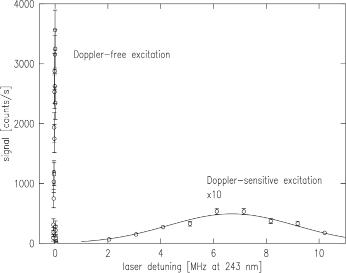
Figure 5-1: Spectrum of non-degenerate gas. The intense narrow peak on the left results from Doppler-free excitation and the low broad peak on the right results from Doppler-sensitive excitation which probes the velocity distribution. The solid line on the right is the expected Doppler-sensitive spectrum for a nondegenerate sample at 42 $\mu$K. At this low temperature the recoil-shifted Doppler-sensitive line is clearly separated from the Doppler-free line. The error bars are statistical. The ratio of peak heights should be taken as only a rough indication of the transition rate ratios because of variations in laser power and beam alignment.

As described in section 5.1.1, there are two components of the spectrum, corresponding to absorption of co- or counter-propagating photons. The wide, low feature on the right (higher photon energy) is the Doppler-sensitive peak, and is offset by the recoil shift $\Delta\nu_{R}$ from the intense, narrow Doppler-free peak on the left. The solid line is the Gaussian lineshape expected for a Maxwell-Boltzmann distribution of kinetic energies in a sample at $42~{}\mu$K. The DS spectrum maps the velocity distribution through the Doppler shift; only atoms with the proper velocity $v=\lambda\Delta\nu$ are Doppler shifted into resonance for a given laser detuning $\Delta\nu=\nu-(\nu_{0}+\Delta\nu_{R})$ ($\nu$ is the optical frequency of the laser). Thus, only a tiny fraction of the sample is resonant, and the excitation rate is correspondingly tiny. The fraction of atoms which are resonant is proportional to the ratio of the excitation linewidth, $\delta_{0}$ from time-of-flight broadening, to the Doppler linewidth $\Delta_{D}=\sqrt{2{k_{B}}T\log(2)/m\lambda^{2}}$; in our apparatus this ratio is $\sim 5\times 10^{-4}$. The very high densities of our trapped samples have allowed us to measure the DS $1S$-$2S$ spectrum of hydrogen for the first time.

The Doppler-free spectrum gives information about the density distribution and temperature of the gas, as described above. Both of these effects are shown by the spectra in figure 5-2,

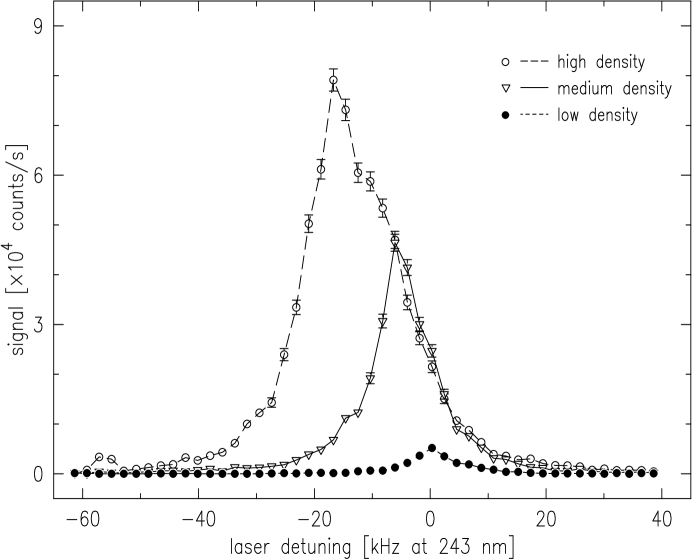
Figure 5-2: Doppler-free spectra at various sample densities. The trap depth is 570 $\mu$K, corresponding to a sample temperature $T\sim 70~{}\mu$K. The spectra of the higher density samples are red-shifted and broadened by the inhomogeneous density. The lines connecting the points are a guide to the eye. The samples were confined by trap shape A, described in table 5.1. The highest density is about $10^{14}~{}{\rm cm^{-}3}$.

just three of many successive spectra that were measured as the density of the sample slowly decayed. The initial spectra exhibit a large shift, arising from the cold-collision frequency shift at high density. The inhomogeneous density in the trap causes a broadening of the spectrum as well. As the sample density decreases, the shift and broadening also decrease. At low density, where the density-dependent shift is negligible, the exponential lineshape characteristic of transit time broadening is evident. The frequency shift of the spectra of high density samples is used to obtain the sample density, and the width of the transit-time broadened line is related to the sample temperature.

5.2 Cooling into the Degenerate Regime

Armed with an efficient cooling method (rf evaporation) and a sensitive probe of sample density and temperature (spectroscopy), we are equipped to push toward the quantum degenerate regime. The trap is loaded as described in section 1.3, and the sample is cooled by magnetic field saddlepoint evaporation. The currents in the magnetic coils that create the trapping potential are ramped to slowly change the trap from the deep, long, open shape used for loading the atoms to a short, tightly compressed, shallow trap from which rf evaporation is commenced. Figure 5-3 indicates the process.

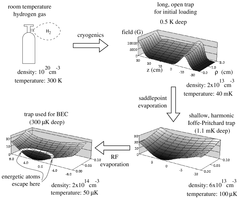
Figure 5-3: Schematic diagram of trap shape as sample is loaded and evaporatively cooled to BEC. Room temperature molecular hydrogen (upper left diagram) is cooled to $275~{}$mK by cryogenic techniques. It is dissociated, and the atoms are loaded into an open, long trap that is about 500 mK deep (upper right diagram). The magnetic field in the $\rho-z$ plane is shown. Note the very different scales for the radial coordinate $\rho$ and the axial coordinate $z$. During trap loading, the atoms settle into the region of low field at the center of the trap. The sample is then cooled by magnetic saddlepoint evaporation. It is compressed radially and axially into a trap that is nearly harmonic along the $z$ axis and predominantly linear along the radial axis (lower right diagram). It is this trap shape that is labeled “A” or “B” (see section 5.2.1). RF evaporation is used to further cool the sample while the trap shape remains fixed (lower left diagram). The entire cooling process takes about 5 minutes.

In this section we discuss the path through density-temperature space taken by the sample as it is cooled into the quantum degenerate regime.

5.2.1 Cooling Paths

Previous attempts to achieve BEC in hydrogen were thwarted by inefficient evaporation at the lowest temperatures. In order to verify that we have solved this problem, the progress of the sample through phase space (density-temperature space) is monitored as the sample is cooled. We find that the sample is cooled efficiently. We also find and explore the phase boundary where the sample undergoes phase separation into a condensate and normal gas. This first evidence for phase transition behavior is described below.

A series of measurements were made to map the sample’s trajectory through phase space as it was cooled into the quantum regime. Identical samples were cooled into a trap of depth $\epsilon_{t}/{k_{B}}=1.1$ mK. This process used magnetic saddlepoint evaporation exclusively. The trap shape was then held constant while the trap depth was reduced by rf evaporation. (Three trap shapes will be discussed in this chapter, A, A^′, and B. Their characteristics are summarized in table 5.1. Here we refer to trap shape A.)

parameter	trap A	trap A′	trap B
$\alpha/{k_{B}}$ (mK/cm)	15.9		9.5
$\beta/{k_{B}}$ ($\mu$K/cm2)	25
$\theta/{k_{B}}$ ($\mu$K)	$27\pm 2$	$35\pm 2$	$34\pm 2$
$n_{0}(T=120~{}\mu$K) ($\times 10^{13}$ cm-3)	8		1.7

Table 5.1: Summary of parameters describing the three trap shapes used in this chapter. The parameters $\alpha$, $\beta$, and $\theta$ describe the Ioffe-Pritchard potential; $\alpha$ and $\beta$ are calculated, and $\theta$ is measured. The peak density at $T=120~{}\mu$K is noted.

The evaporation path (the trap depth as a function of time) was identical for all samples, but the different samples were taken various distances along the path. The rf frequency $f(t)$ that sets the trap depth ${\epsilon_{t}}=hf(t)-\theta$ was ramped according to the function $f(t)=f_{start}(f_{end}/f_{start})^{(t/d)^{\xi}}$ where the start frequency is $f_{start}=23$ MHz, the end frequency is $f_{end}=2$ MHz, the maximum ramp duration is $d=25$ s, and the shape exponent $\xi=1.5$. The ramp was executed for a duration $\tau_{r}$. For $t\geq\tau_{r}$, the frequency was maintained at $f(\tau_{r})$. Evaporation could still occur, but forced evaporation halted. After rf evaporation was completed, the sample density was measured using the cold-collision frequency shift of the DF spectrum as described above. The densities thus measured are shown in figure 5-4.

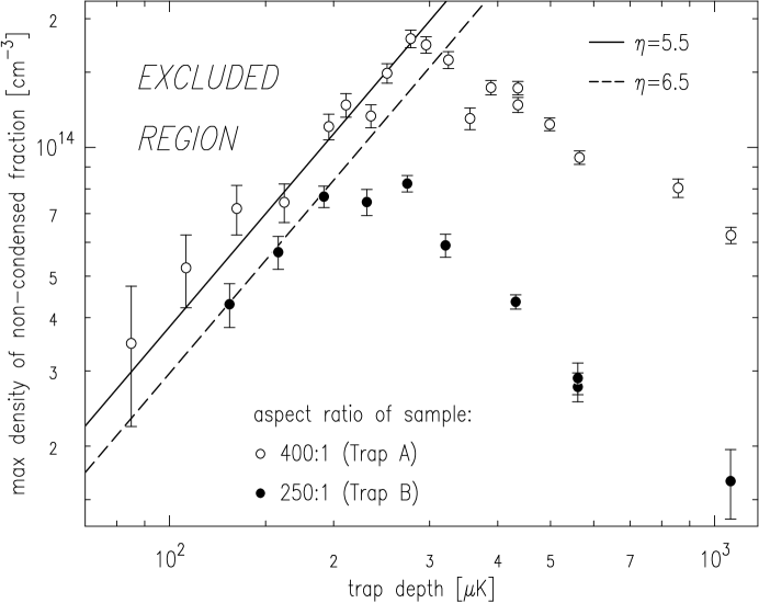
Figure 5-4: Path of non-condensed portion of the sample through $n-T$ space as the sample is cooled into the degenerate regime. Paths are shown for samples in two different traps: open circles — trap A, closed circles — trap B. The trap depth is set by the frequency of the rf magnetic field, and above degeneracy the temperature is about $1/\eta\sim 1/8$th the trap depth. The density is measured through the cold-collision frequency shift. The non-condensed portion of the sample cannot have density greater than the BEC critical density $n_{c}\propto T^{3/2}$, and thus the upper left region of the phase diagram is not accessible. The condensates created in the two traps contain about the same number of atoms.

The density initially increases as the trap depth (and thus temperature) is reduced because the atoms are confined to a smaller volume closer to the bottom of the trap. Some atoms are lost through evaporation, but the good efficiency of evaporative cooling leads to overall phase space compression. The cooling efficiency parameter $\gamma=d\log D/d\log N$ (the phase space density is $D\equiv n_{0}\Lambda^{3}$) is $\gamma\simeq-1.5$ during this stage of the cooling.

At a trap depth of about $\epsilon_{t}/{k_{B}}=280~{}\mu$K the phase space trajectory exhibits a dramatic kink. Further cooling leads to decreasing density in the normal gas; apparently population is being rapidly removed. The location of the kink and the slope of the subsequent trajectory agree well with the BEC phase transition line, $n_{c}=2.612(2\pi m{k_{B}}T)^{3/2}/h^{3}$ assuming a ratio of trap depth to temperature of $\eta=\epsilon_{t}/{k_{B}}T\sim 6$, which is reasonable. The “excluded region” above the line has the following interpretation: as the sample is cooled, the thermal cloud cannot support a peak density above $n_{c}$; extra atoms are transferred to the condensate. The condensate is not directly observed in these measurements because its density is so large (as discussed in section 5.3.1) that its spectrum is shifted far away from the spectrum of the thermal cloud.

The magnetic trap shape used for these experiments (trap shape A) was chosen as a compromise between high radial compression and adequate magnetic saddlepoint evaporation efficiency. High radial compression is desirable because the correspondingly higher densities allow BEC to be reached at a higher temperature. As discussed in section 5.2.2, evaporation and the approach to BEC should be more efficient at higher temperatures because the ratio of “good” to “bad” collisions is more favorable. On the other hand, high radial compression is undesirable because the magnetic field saddlepoint evaporation process (see figure 5-3) that cools and compresses the sample into the tight trap is less efficient. As discussed in section 2.1, tight radial compression leads to more regular motion of the trapped atoms, and thus to reduced evaporation dimensionality.

A more open trap, trap B, has also been used. A typical phase space trajectory is shown by the filled circles in figure 5-4 . The evaporation was done more slowly, with maximum duration $d=55$ s, but was otherwise identical to the path described above. The evaporation efficiency parameter is $\gamma\sim-2.7$ for cooling above the degenerate regime. The higher evaporation efficiency has not been systematically studied, but could arise simply because the trajectory duration $d$ was optimized for trap B, but not trap A.

Computer models of the cooling process have been constructed, and are described in appendix D. The trajectories through phase space calculated by them are in good agreement with observations.

5.2.2 Evaporation Strategies

There are many paths that can be taken through phase space to the BEC phase boundary. In this section we discuss the experimental limitations of the present apparatus and their implications for the choice of evaporation path.

As shown in section A.2.2, evaporation is more efficient in hydrogen at higher temperatures. There the ratio of “good” collisions to “bad” collisions is higher. “Good” collisions are those which lead to cooling, and they occur at a rate $\Gamma_{evap}\propto\Gamma_{col}\propto n\sigma\bar{v}\propto n\sqrt{T}$ for a sample of density $n$. “Bad” collisions are those which lead to dipolar relaxation and heating. They occur at a rate $\Gamma_{dip}\propto gn$. The collision ratio $\Gamma_{evap}/\Gamma_{dip}\propto\sqrt{T}$ is higher at higher temperatures. More phase space compression can be accomplished per atom lost from the trap. This higher efficiency makes it desirable to do most of the phase space compression at higher temperatures.

The competing consideration is that full evaporation dimensionality, and thus efficiency, can only be realized using the rf evaporation technique (instead of saddlepoint evaporation), and this technique is only usable for trap depths less that about 1 mK. Creation of deeper traps requires higher frequency and higher power rf fields. These heat the current apparatus too much.

In an ideal apparatus the rf evaporation would be initiated at much higher temperatures, phase space compression would lead to higher sample densities, and the bulk of the cooling and compression would be accomplished more quickly and more efficiently than in the present experiments. The sample could then be cooled at nearly constant phase space density to cross the BEC phase transition line at the desired density (one may desire smaller densities with correspondingly longer lifetimes). In the experiments described here more phase space compression was accomplished at lower temperatures than is optimal because of the heating effects of the rf power used for evaporation. Improvements to the rf parts of the apparatus should allow larger condensates to be created.

To test these ideas about efficiency we cooled to BEC in two traps, A and B described above. (These labels refer to the field configuration at low temperature. Identical trap shapes are used for initial trap loading ($T=40$ mK, $n_{0}=2\times 10^{13}~{}{\rm cm^{-3}}$) and the first stage of saddlepoint evaporative cooling. The trap shape is converted into A or B during the last stage of the saddlepoint evaporation.) The evaporation occurred along different paths for the two traps, but at the end the phase space density was nearly identical; the condensate population was about $10^{9}$ atoms for both traps. One expects path B to have lower overall evaporation efficiency (and thus fewer condensate atoms) because more of the phase space compression is accomplished at lower temperatures (where the evaporation efficiency is lower because the ratio of good to bad collisions is less favorable). On the other hand, if rf evaporation is more efficient than saddlepoint evaporation, then one expects path B to result in better evaporation efficiency, and thus more condensate atoms, since more of the phase space compression is accomplished with the more efficient rf evaporation. Since the two paths result in the same final phase space density, we conclude that the two effects cancel. This necessitates that rf evaporation be more efficient than saddlepoint evaporation. It would be advantageous to use rf evaporation for more of the cooling.

5.3 Spectroscopic Study of the Degenerate Gas

When the sample is cooled into the quantum degenerate regime we observe signatures of the condensate in the $1S$-$2S$ spectrum of the gas. In this section we discuss two of these signatures from which we extract the chemical potential and temperature. Knowledge of these thermodynamic parameters allows us to estimate several properties of the system.

Bose condensation involves the macroscopic occupation of the lowest energy quantum state of the system. In a trap this state is concentrated at the minimum of the trapping potential, and it has very small kinetic energy, given approximately by the Heisenberg momentum-position uncertainty principle. In the Doppler-sensitive spectrum, which maps the momentum distribution, one would expect an intense line at zero detuning from the recoil shift $\Delta\nu_{R}$, rising above the background spectrum [16]. Figure 5-5 shows the DS spectrum of the normal gas and the condensate together.

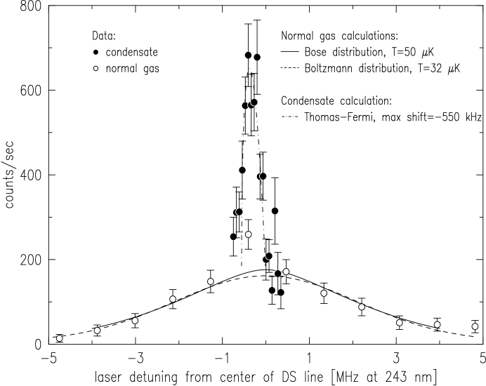
Figure 5-5: Doppler-sensitive spectrum of degenerate gas. Zero detuning is taken at center of the recoil-shifted spectrum, which is detuned 6.70 MHz blue of the Doppler-free resonance. open circles—normal gas, filled circles—spectrum focusing on condensate. The dashed line is a fit to the normal fraction data which assumes a Maxwell-Boltzmann velocity distribution. The solid line is a calculation which assumes a Bose-Einstein distribution. The dot-dashed line is the condensate spectrum expected for a Thomas-Fermi wavefunction in a harmonic trap, when the dominant spectral broadening is the cold-collision frequency shift. The temperature of the Bose calculation was chosen to fit the observed spectrum. The condensate spectrum is a composite of data from the first sweep of each of three loadings of the trap; the spectral sweep took 0.94 s. The normal spectrum is a composite of data from the first three sweeps of each of two loadings of the trap; the spectral sweep took 0.94 s. This data is for trap shape B.

Instead of appearing as a very narrow, intense peak centered at zero detuning, however, the line is red-shifted and broadened by the very high and inhomogeneous density of the condensate. This same effect is observed in the DF line, displayed in figure 5-6.

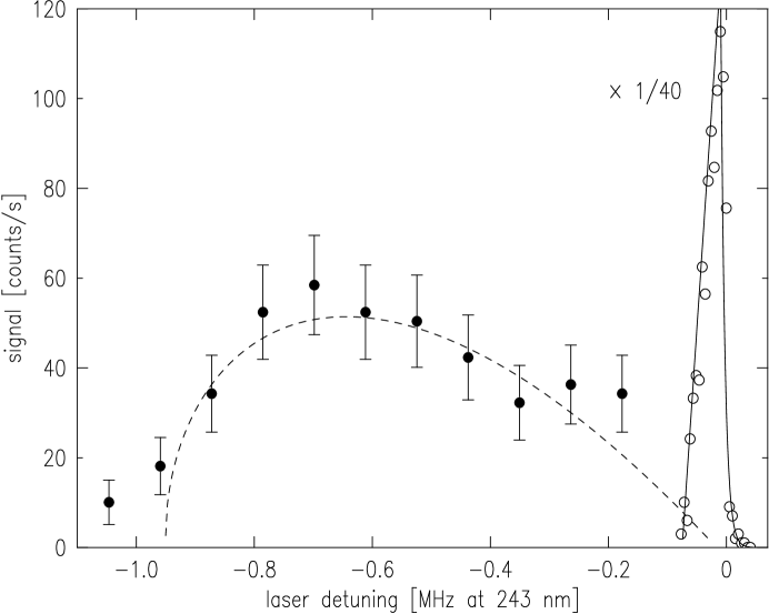
Figure 5-6: Doppler-free spectrum of degenerate gas. The intense, narrow feature on the right is due to the normal gas, and is shrunk vertically by a factor of 40 to fit in the plot. The wide, low, red-shifted feature is the condensate. The lineshape is that expected for a Thomas-Fermi wavefunction in a harmonic trap. The spectrum is a composite of the first two spectral sweeps from each of 10 loadings of the trap; the sweep took 0.67 s. The normal gas spectrum is a single sweep from a single loading of the trap. This data is for trap shape A^′.

The condensate spectrum has a very different shape and shift than the normal gas spectrum, implying very high densities and a density distribution that is different from the normal gas.

The spectroscopic technique of probing the condensate differs significantly from the spatial imaging techniques used by other groups, providing somewhat complementary information. The probe is not limited to length scales larger than the spatial resolution of the imaging optics, and so detection of very small features, such as condensate “droplets” [93] would be possible. Also, we are able to measure the momentum distribution of the normal gas in situ. Finally, the coherence length of the condensate can, in principle, be obtained directly from the broadening of the spectrum, as recently demonstrated in Na by Stenger et al. [94]. Because of the large condensate densities, we are only able to put a very small lower bound on the coherence length for our H condensates.

5.3.1 Peak Condensate Density

The DF spectrum of the condensate, shown in figure 5-6, can be understood using a local density approximation; atoms excited from different regions of the condensate exhibit correspondingly different frequency shifts. The signal size $S$ at a given detuning $\Delta$ is proportional to the number of condensate atoms on a surface of constant density $n_{cond}=2\Delta/\chi_{c}$, where $\chi_{c}$ is the (two photon sum) frequency shift per unit density for excitation out of the condensate. (The relation of $\chi_{c}$ to $\chi_{m}$, the measured [7] frequency shift per unit density for excitation out of the thermal gas quoted in equation 5.3, will be addressed in section 5.6. Although there is significant ambiguity, it is clear that either $\chi_{c}=\chi_{m}$ or $\chi_{c}=\chi_{m}/2$.) The spectrum calculated using this local density approximation in a harmonic potential is parameterized only by the peak shift, $\Delta_{p}$, and the overall scaling factor $S_{0}$. The normalized spectrum is

$$S(\Delta)=\left\{\begin{array}[]{lll}S_{0}\frac{-15\Delta}{4(-\Delta_{p}^{5/2})}\sqrt{\Delta-\Delta_{p}}&;&\Delta_{p}\leq\Delta\leq 0\\ 0&;&{\rm otherwise}\end{array}\right..$$ (5.4)

(The negative signs are appropriate for red density shifts: $\Delta_{p}<0$.) A fit of this function to the measured spectrum is the dashed line in figure 5-6. The peak shift is $920\pm 70$ kHz, which indicates a peak condensate density $n_{p}=2\Delta_{p}/\chi_{c}=4.8\pm 0.4\times 10^{15}~{}{\rm cm^{-3}}$ (assuming $\chi_{c}=\chi_{m}$; the uncertainty reflects the statistical fitting uncertainty, and ignores the 20% uncertainty in $\chi_{m}$). If we assume $\chi_{c}=\chi_{m}/2$ the density is twice as big. The quality of the fit indicates the utility of the Thomas-Fermi wavefunction approximation.

A quantum mechanical approach may also be used to understand this spectrum, as developed in the thesis of Killian [13]. Before excitation, an atom is in the $1S$ electronic state, and its motional quantum state is the condensate wavefunction. After excitation the atom is in the $2S$ electronic state; its motional state has been projected onto the motional eigenstates of the modified potential it experiences. This new potential, a sum of the trap potential and the mean-field interaction energy for a $2S$ atom in a $1S$ cloud, is very different because the new mean-field energy has a different sign and is much stronger. The parabolic condensate density profile, with density much larger than the background thermal cloud density, gives rise to an attractive parabolic potential for the $2S$ atoms. The motional quantum states the $2S$ atom finds available are simple harmonic oscillator states. The excitation spectrum is the probability of exciting atoms from the condensate wavefunction to each of these $2S$ motional states. This probability is the wavefunction overlap, which is straightforward to calculate. Calculations by Killian show very good agreement between the quantum and local density approximation treatments of the spectrum.

The peak condensate density indicates the number of atoms in the condensate, given a knowledge of the trap shape. (This data is for trap shape A^′). Using equation 2.14 we obtain $N_{c}=1.2\pm 0.2\times 10^{9}$. This is larger by a factor of 50 than the biggest condensate created so far in other labs [95]. Using equation 2.15, the characteristic dipolar decay rate is $\Gamma_{2,c}=\dot{N}_{2,c}/N_{c}=1.7~{}{\rm s}^{-1}$. The chemical potential for this peak density is $\mu=n_{p}U_{0}=1.9~{}\mu$K. The extent of the Thomas-Fermi wavefunction is determined from equation 2.13 by setting the density to zero at the edge of the condensate: $n_{cond}U_{0}=\mu-V_{IP}(\rho,z)=0$. We obtain

$$\rho_{max}=\frac{1}{\alpha}\sqrt{\mu^{2}+2\mu\theta}=7.3~{}\mu{\rm m}$$ (5.5)

and

$$z_{max}=\sqrt{\frac{\mu}{\beta}}=2.8~{}{\rm mm}.$$ (5.6)

For trap B, similar data has been obtained. The peak shift of $\Delta_{p}=620\pm 20$ kHz corresponds to a peak density $3.26\pm 0.10\times 10^{15}~{}{\rm cm^{-3}}$ (assuming $\chi_{c}=\chi_{m}$; the uncertainty reflects the statistical fitting uncertainty, and ignores the 20% uncertainty in $\chi_{m}$). In this more open trap, the condensate population is $N_{c}=1.19\pm 0.10\times 10^{9}$, the chemical potential is $\mu/{k_{B}}=1.28\pm 0.04~{}\mu$K, the diameter is $2\rho_{max}=20~{}\mu$m, and the length is $2z_{max}=4.5$ mm. If we assume $\chi_{c}=\chi_{m}/2$, then the peak density is twice as high, and the derived condensate parameters are correspondingly different. These results are summarized in table 5.2.

parameter	trap A′		trap B
$\alpha/{k_{B}}$ (mK/cm)	15.9		9.5
$\beta/{k_{B}}$ ($\mu$K/cm2)	25		25
$\theta/{k_{B}}$ ($\mu$K)	$35\pm 2$		$34\pm 2$
${\epsilon_{t,c}}/{k_{B}}$ ($\mu$K)	280		220
${\epsilon_{t}}/{k_{B}}$ ($\mu$K)	272		214
$T_{c}$ ($\mu$K)	$\sim 65$		$\sim 50$
$\Delta_{p}$ (kHz)	$920\pm 70$		$620\pm 20$
	$\chi_{c}=\chi_{m}$	$\chi_{c}=\chi_{m}/2$	$\chi_{c}=\chi_{m}$	$\chi_{c}=\chi_{m}/2$
$n_{p}$ ($\times 10^{15}$ cm-3)	$4.8\pm 0.4\pm 1$	$9.7\pm 0.7\pm 2$	$3.3\pm 0.1\pm 0.7$	$6.5\pm 0.2\pm 1.3$
$\mu/{k_{B}}$ ($\mu$K)	1.9	3.8	1.3	2.6
$N_{c}$ ($\times 10^{9}$)	$1.2\pm 0.2(^{+0.7}_{-0.5})$	$6.6\pm 1.3(^{+4}_{-3})$	$1.2\pm 0.1(^{+0.7}_{-0.5})$	$6.7\pm 0.5(^{+4}_{-3})$
$\Gamma_{2,c}$ (s-1)	1.7	3.3	1.1	2.2
$2\rho_{max}$ ($\mu$m)	15	21	20	28
$2z_{max}$ (mm)	5.5	7.8	4.5	6.4

Table 5.2: Summary of parameters describing the two trap shapes used for achieving BEC, and summary of the properties of the condensates. The parameters $\alpha$, $\beta$, and $\theta$ describe the Ioffe-Pritchard potential; $\alpha$ and $\beta$ are calculated, and $\theta$ is measured. The trap depth at which BEC is first observed is ${\epsilon_{t,c}}$, and the trap depth used for the observations listed here is ${\epsilon_{t}}$. The approximate temperature in the presence of the biggest condensates is $T_{c}$. The peak cold-collision frequency shift in the condensate is $\Delta_{p}$. The remainder of the table is divided to show the implications of assuming $\chi_{c}=\chi_{m}$ or $\chi_{c}=\chi_{m}/2$ (recall the sum frequency shift is $\chi_{m}=-3.8\pm 0.8\times 10^{-10}~{}{\rm Hz~{}cm^{3}}$). The peak condensate density is $n_{p}$, and the chemical potential is $\mu$. The number of condensate atoms is $N_{c}$. The characteristic condensate dipolar decay rate is $\Gamma_{2,c}=\dot{N}_{2,c}/N_{c}$. Finally, the length and diameter of the condensates are given. The uncertainties are divided into a component which depends on the present experiment (first number), and a component reflecting the 20% uncertainty on $\chi_{m}$ (second number).

5.3.2 Sample Temperature

The temperature and chemical potential of the trapped gas allows a full thermodynamical description of the system, assuming a near equilibrium situation. The chemical potential was obtained above. The temperature is extracted here using two methods, both of which suffer from uncomfortably large uncertainties. Nevertheless, in this section we characterize the temperature with uncertainty on the 20% level.

The primary thermometry tool is the DS spectrum of the normal gas. As described in section 5.1.1 above, the spectrum is a map of the velocity distribution of the sample. Far from quantum degeneracy this (classical) velocity distribution is Gaussian, and the normalized spectrum is

$$S(\Delta)=\frac{S_{0}}{\sigma\sqrt{2\pi}}\exp\left(-\frac{\Delta^{2}}{2\sigma^{2}}\right)$$ (5.7)

where $\sigma=\sqrt{{k_{B}}T/m\lambda^{2}}=373.6\sqrt{T/1~{}\mu{\rm K}}$ kHz is the linewidth parameter and the detuning $\Delta$ is measured in Hz. We have not measured the DS spectrum of the gas far from quantum degeneracy because the low sample density reduces the signal rate below the background noise. There is sufficient signal near the degenerate regime, however. For a degenerate Bose gas at a given temperature, the velocity distribution is significantly narrower than its classical counterpart because the particles are distributed toward lower energies. In a homogeneous potential the DS spectrum of an ideal gas is cusp-shaped:

$$S(\Delta)\propto\log\left[1-\exp\left(\frac{\mu-\frac{\lambda^{2}\Delta^{2}m}{2}}{{k_{B}}T}\right)\right].$$ (5.8)

In a trap, however, only the atoms at the very bottom of the trap are in the quantum degenerate regime. Atoms in regions of potential energy $\varepsilon\geq{k_{B}}T$ experience a reduced phase space density, parameterized by an effective chemical potential $\mu^{\prime}=(\mu-\varepsilon)\leq-1{k_{B}}T$; their velocity distribution is nearly classical. The measured spectrum is an average over the various velocity distributions in the gas. Appendix E presents a detailed treatment of Doppler-sensitive optical excitation in a trap, showing that if the laser beam is small, then atoms in regions of high phase space density are preferentially excited and the spectrum reflects the Bose velocity distribution more dramatically. The shot noise on our measurements is too big to allow a precise comparison between the shapes of the classical and quantum spectra, but evidence of the effect is noted in the spectrum below.

Although it is interesting to probe the Bose-Einstein velocity distribution and compare it to the Maxwell-Boltzmann, the disadvantage presented by the effect is the dependence of the spectrum on the effective chemical potential, which leads to measurement uncertainties. The laser beam geometry and alignment must enter the interpretation of the spectrum, and these factors are difficult to measure directly. The alignment of the beam with the sample is verified by translating the trap radially relative to the laser beam while exciting the condensate. The condensate is used as a precise alignment marker in the center of the trap. With this technique we can center the trap radially over the laser beam to within about a half a beam radius (20 $\mu$m), small compared to the thermal radius of the normal gas (100 $\mu$m). Systematic axial adjustment is not possible in the current apparatus. The uncertainty in the axial position of the beam focus is about 2 cm, about half the length of the normal gas cloud.

To demonstrate the technique we study here the DS spectrum of a sample in trap B, in the quantum degenerate regime. Plotted in figure 5-7 is the DS spectrum, obtained immediately after forced rf evaporation is completed; the trap depth is ${\epsilon_{t}}=214~{}\mu$K.

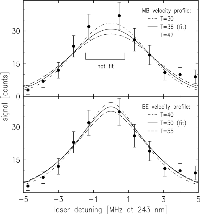
Figure 5-7: Doppler-sensitive spectrum of degenerate gas. The condensate signal (point at -0.5 MHz detuning) is off scale. In the upper panel the wings of the line (all points except center three) are fit to a Gaussian, the expected lineshape for a Maxwell-Boltzmann (MB) velocity profile. The fit temperature is $T=36\pm 6~{}\mu$K. In the lower panel the same data is compared to calculations of the spectrum which assume a Bose-Einstein (BE) velocity distribution for a degenerate gas in trap B. Spectra calculated for three temperatures are displayed. We conclude that the sample temperature is $T=50\pm 10~{}\mu$K, corresponding to $\eta=4.3\pm 0.9$. The BE velocity distribution fits the low velocity portion of the data better than the MB distribution, indicating the presence of quantum effects in the momentum distribution. The data is compiled from the first three sweeps of two samples; each sweep required 0.94 s.

The first step in the analysis is to fit the wings of the spectrum with a Gaussian, an analytic form that is simple to fit. This fit is shown in the upper panel along with the spectra expected for temperatures higher and lower than the fit result by one standard deviation. Next, spectra are calculated assuming a truncated Bose-Einstein velocity distribution, as described in appendix E. These calculations take into account the trap shape, trap depth, laser beam waist, and alignment of laser beam relative to the center of the trap (we choose ideal alignment here: beam focus at center of trap, beam aligned with the $z$ axis). The calculations are done for a range of temperatures. The calculated spectra are fit in the wings by a Gaussian, and the spectrum with fit temperature closest to the fit temperature of the data is chosen. For the data in figure 5-7, the fit temperature for the data is $36\pm 6~{}\mu$K. The calculated Bose spectrum with temperature $T=50~{}\mu$K also had a fit temperature of 36 $\mu$K (see below). This spectrum, and those for $T=40~{}\mu$K and $55~{}\mu$K are plotted in the lower panel of figure 5-7. We conclude that the sample temperature is $T=50\pm 10~{}\mu$K.

When a Gaussian is fit to a Bose velocity distribution, calculated for temperature $T_{BE}$, the fitted temperature $T_{MB}$ is significantly lower than $T_{BE}$ because of two effects. First, the Bose distribution concentrates population at the low energies corresponding to the low velocity area near the center of the spectrum. This effect is tuned by changing the chemical potential from the quantum degenerate regime ($|\mu|\ll{k_{B}}T$) to the classical regime ($|\mu|\gg{k_{B}}T$, $\mu<0$). The fit temperature is also smaller than $T_{BE}$ because the true energy distribution is truncated, and the Gaussian profile disregards truncation. This effect is tuned by changing the trap depth parameter $\eta\equiv{\epsilon_{t}}/{k_{B}}T_{BE}$ (in practice ${\epsilon_{t}}$ is fixed and $T_{BE}$ is varied). For large $\eta$ truncation is unimportant, while for the small $\eta$ values used here truncation effects cause significant deviations. The calculation procedure has been checked in these limits.

A systematic error can arise if the laser beam focus is not aligned in the trap as expected. The beam would be probing a region with effective chemical potential different from expected. Three beam parameters affect the alignment: the beam waist, the radial position of the beam, and the axial position of the beam. We know the waist radius to within 30% because of the aperture constraints encountered while transporting the beam into the cryostat and back out. The radial position of the beam is measured by translating the trap, and is verified by the presence of the condensate spike in the center of the spectrum. The axial position of the beam is not as important because the divergence length is on the order of the length of the sample. We conclude that uncertainties in the beam parameters should not cause a major systematic effect compared to the shot noise of the current measurements.

The other indication of sample temperature comes from the phase space diagram, figure 5-4. For trap B, the phase boundary appears at a ratio of trap depth to temperature of $\eta\simeq 6.5$. This would indicate that the temperature of the sample in figure 5-7 should be 33 $\mu$K. A systematic error arises, however, in the extraction of the peak density of the normal gas (plotted in figure 5-4) from the DF spectra. The lineshape of the spectrum changes significantly near the onset of quantum degeneracy, as detailed in section 5.5. This systematic error could shift the apparent density higher by up to roughly 30% (measured density higher than actual density), translating to a decrease in the indicated temperature by 20% (measured temperature lower than actual temperature). This adjustment shifts the expected sample temperature to $40~{}\mu$K, within the uncertainty of the DS measurement.

We note that the DS spectrum does not constitute an absolute measure of the sample temperature in the regimes of quantum degeneracy and/or shallow traps (low $\eta$). On the contrary, the details of the trap shape and laser beam geometry are folded into the spectrum. In spite of these difficulties, reliable temperatures can be extracted. In addition, we observe in figure 5-7 hints of quantum perturbation of the momentum distribution of the normal gas, a subject which could be studied with improved signal rate.

Our temperature derivation procedure could be complicated by a non-uniform temperature in the sample. Loss of atoms from the trap occurs mostly in the condensate when the condensate density is high. As explained in section 2.3.2.1, the effective heating rate of the system is thus higher in the center 10% of the length of the trap where the condensate lives. Near the ends of the thermal gas the heat load is lower, and conceivably the temperature could be lower.

In order for a temperature gradient to exist, the characteristic mean free path must be less than the length of the sample. At the highest densities achieved, the thermal gas has peak density $n_{0}=2\times 10^{14}~{}{\rm cm^{-3}}$ corresponding to a mean free path $l=1/n_{0}\sigma\simeq 4$ cm. This is about the characteristic length of the sample. While significant thermal gradients are not expected, there is a danger of such effects.

5.3.3 Condensate Fraction

The fraction of atoms in the condensate can be obtained using two methods. First, given knowledge of the trap shape and sample temperature, we compute the population of the normal gas using equation C.7 (which assumes thermal equilibrium). We then compare to the condensate population computed above using equation 2.14. The trap shape parameters $\alpha$ and $\beta$ cancel in the comparison, and the only quantities that enter are measured: the temperature, peak condensate density $n_{p}$, and trap bias energy $\theta$. The population ratio $f=N_{c}/N_{t}$ is given by equation 2.18. We use $f$ to plot the condensate fraction, $F=f/(1+f)$, in figure 5-8 for the trap depth, bias energy, and range of temperatures applicable to trap B.

Figure 5-8: Condensate fraction $F=f/(1+f)$ as a function of sample temperature, plotted for various bias energies. The heavy lines correspond to peak condensate density $n_{p}=3.3\times 10^{15}~{}{\rm cm^{-3}}$, and the light lines correspond to a peak density twice as big. The trap depth corresponds to trap B, as do the solid lines ($\theta/{k_{B}}=35~{}\mu$K). A temperature of $50~{}\mu$K indicates a condensate fraction around 2% (12%) for $\chi_{c}=\chi_{m}$ ($\chi_{c}=\chi_{m}/2$). The calculations, based on equation 2.18, properly treat the finite trap depth.

The condensate fraction for trap B corresponding to $T=50\pm 10~{}\mu$K is $F=f/(1+f)=2.4(^{+2}_{-1})(^{+1.4}_{-1})$% (uncertainties arising from $T$ and $\chi_{m}$ listed separately). This is in agreement with estimates by Hijmans et al. [45].

We have found the condensate fraction just after crossing the BEC phase boundary; condensate fractions could be determined at other points on the phase diagram, but the high loss from the condensate depletes the system as lower temperatures are attained, reducing the achievable fraction. Also, we are considering equilibrium condensate fractions. As explained in section 5.4, the condensate is fed from the thermal cloud. An extremely high condensate fraction could be created by simply removing all the thermal atoms by rf ejection, but the resulting condensate would decay rather quickly.

The other method of finding the condensate fraction exploits the spectrum more directly; the population of the normal gas is proportional to the integrated signal of the normal component of the DF (or DS) resonance. This integral is compared to the integral of the condensate portion of the spectrum, and adjustments are made to account for the partial illumination of the normal gas by the laser beam. (The condensate diameter is significantly smaller than the beam diameter, but the normal gas diameter is significantly larger.) The fraction computed with this technique [13] is $2.2^{+1}_{-0.5}$%. The two methods give consistent results; an increased signal rate would reduce the large temperature uncertainties and make the measurements useful.

5.4 Time Evolution of the Degenerate Gas

Because the condensate fraction is small, there are enough atoms in the normal gas to continuously replenish the condensate for many seconds. As a first look at this feeding process we study the time evolution of the condensate.

Simple estimates of time scales reveal that the condensate lives much longer than one might expect in the absence of replenishment. The large condensate density leads to fast condensate decay. The characteristic time an atom spends in the condensate before undergoing an inelastic collision is $\tau_{2,c}=N_{c}/\dot{N}_{2,c}$, less than a second for the condensates described in table 5.2. However, the condensate is observed to live for more than $15\tau_{2,c}$, indicating that feeding of the condensate by the thermal cloud occurs quickly. In this section we examine the time evolution of the condensate. We find that a simple equilibrium model reproduces the data.

To measure the condensate dynamics many sequential condensate spectra have been measured. Figure 5-9 shows part of a series of such spectra, obtained using DS absorption, for trap B.

Figure 5-9: Time evolution of the Doppler-sensitive spectrum of the condensate in trap B. Spectra are obtained sequentially after forced rf evaporation is finished. This data is compiled from five identical loadings of the trap. The solid line is a model which is fit to the entire sequence of spectra, only four of which are shown here. [92]

The solid curve is a fit to all the data in the series, with adjustable parameters being the peak condensate density in each scan, the overall amplitude scaling factors for the condensate and normal gas, the temperature of the sample, and a time constant for the temperature to change [92]. The peak condensate density decreases only slowly in time, implying feeding of the condensate from the normal gas. For this feeding to occur, the normal gas must be losing atoms, and thus density. In order for the normal gas to remain on the phase boundary, the temperature must therefore be decreasing.

The time evolution of the condensate can also be probed using the DF spectrum, as shown in figure 5-10.

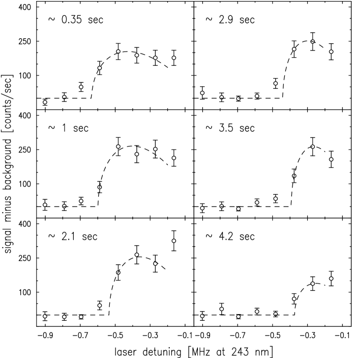
Figure 5-10: time evolution of Doppler-free spectrum of condensate in trap B. The noted time is measured from the end of the forced evaporative cooling cycle to the middle of the sweep. Each spectrum is fit independently with a two parameter model: the peak density $\Delta_{p}$ and an overall scaling factor $S_{0}$; the background is estimated independently. The right side is not fit because of signal spillover from the very intense DF normal line (not shown). This data is a compilation of sweeps from each of five identical loadings of the trap.

Similar results are obtained. Note the systematic misfit of points just to the red of the peak shift, $\Delta_{p}$ in figures 5-10 and 5-6. The spectra suggest that the density distribution of the condensate is more complicated than that predicted by the Thomas-Fermi wavefunction alone. Unfortunately, the low signal rate precludes further study at this time.

Figure 5-11 shows the peak condensate density as a function of time, obtained in two ways.

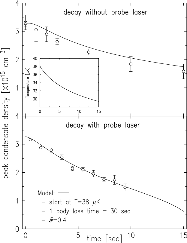
Figure 5-11: Time evolution of peak density of the condensate in trap B. The lower panel shows the peak condensate density extracted from a sequence of DS spectra, some of which are shown in figure 5-9. The upper panel is the peak condensate measured after waiting various times between the end of the forced evaporation cycle and the beginning of the laser scans. This data demonstrates the lifetime of the condensate when the only loss mechanism is dipolar relaxation. The solid lines are from a model of the heating and cooling processes in the normal gas and condensate. For the lower panel a one-body loss rate was introduced. The inset shows the calculated sample temperature evolution in the absence of extraneous atom loss due to the presence of the probe laser.

In the lower panel sequential spectra are taken of the same condensate, and so losses induced by the laser beam cause the sample to decay more quickly than it would without the extraneous one body loss rate. The upper panel reveals the latter situation. Here the sample is held for various intervals after forced rf evaporation is finished, before laser probing is commenced. The sequence of spectra obtained is fit, and a peak condensate density at the beginning of the laser scan is obtained. This density is plotted in the figure. We see that the laser probe shortens the condensate life by only a small factor. We also observe that in the absence of losses induced by the laser, the condensate density decays by only a factor of 2 over 15 s (population decays by factor of $2^{5/2}\simeq 6$).

The number of atoms lost from the condensate through dipolar decay during this interval $d=15~{}$s can be easily estimated by integrating equation 2.15:

$$N_{c,lost}=\int_{0}^{d}dt\;\dot{N}_{2,c}=\frac{16}{105}\>\frac{g}{2!}\varrho_{0}\theta U_{0}^{3/2}\int_{0}^{d}dt\;n_{p}^{7/2}(t)$$ (5.9)

We estimate $N_{c,lost}=6(^{+0.7}_{-0.6})(^{+6}_{-3})\times 10^{9}$ (uncertainties from present experiment and 20% uncertainty in $\chi_{m}$, respectively). If we had used $\chi_{c}=\chi_{m}/2$ this loss would have been $2^{7/2}\simeq 11$ times larger, or $N_{c,lost}=7(^{+0.8}_{-0.7})(^{+6}_{-4})\times 10^{10}$. For a temperature of $50\pm 10~{}\mu$K we estimate a normal gas population of $N_{t}=5^{+3}_{-2}\times 10^{10}$. The spectra show that even after losing $N_{c,lost}$ atoms the trap still contains a sizeable condensate and normal gas. It therefore appears unphysical for $\chi_{c}=\chi_{m}/2$; however, more data should be collected to reduce the large uncertainties in this measurement.

A computer model has been developed to study the time evolution of the degenerate system. As described in appendix F, this model incorporates dipolar decay and evaporative cooling, and assumes thermal equilibrium and a Thomas-Fermi condensate wavefunction. The good agreement between the model (solid line in figure 5-11) and the data indicates that the system is reasonably well understood. An important result of the model is that the temperature of the sample changes by 20-30% during the 15 s condensate lifetime. This behavior is shown in the inset to figure 5-11.

The low condensate fraction and long condensate lifetime in this system suggest that the H condensate could be an excellent source for a bright atom laser. On the order of $10^{8}$ atoms/s could be continuously coupled out of the condensate for 10-20 s per loading of the trap (continuous loading schemes could be imagined to circumvent this limitation). The outcoupling could be accomplished by photon recoil as atoms are excited to the $2S$ state [25] or by Raman output coupling, as demonstrated in Na by Kozuma et al. [96]. The beam thus formed should be diffraction limited; the large condensate dimensions and short de Broglie wavelengths achievable in this system should result in a very low divergence beam. The atoms in the beam could be in the metastable $2S$ state, which could be useful because of the large energy available for driving chemistry on a surface the atoms hits.

5.5 Signature of Quantum Degeneracy in Spectrum of Normal Gas

The direct condensate signatures presented so far are expected from simple theories of BEC. One does not expect the DF spectrum of the normal gas to be much affected by the condensate. Nevertheless, a dramatic signature appears.

Simple arguments suggest that the for this experiment ($\mu\ll{k_{B}}T$) the normal gas should be only very weakly perturbed by quantum degeneracy. The condensate volume is about a factor of $10^{3}$ smaller than the volume of the normal gas, so the high condensate density should not affect the normal gas much.

In fact, measurements of the DF spectrum of the normal gas in the degenerate regime reveal a surprise. The lineshape is markedly asymmetric below the transition, but largely symmetric above, as shown in figure 5-12.

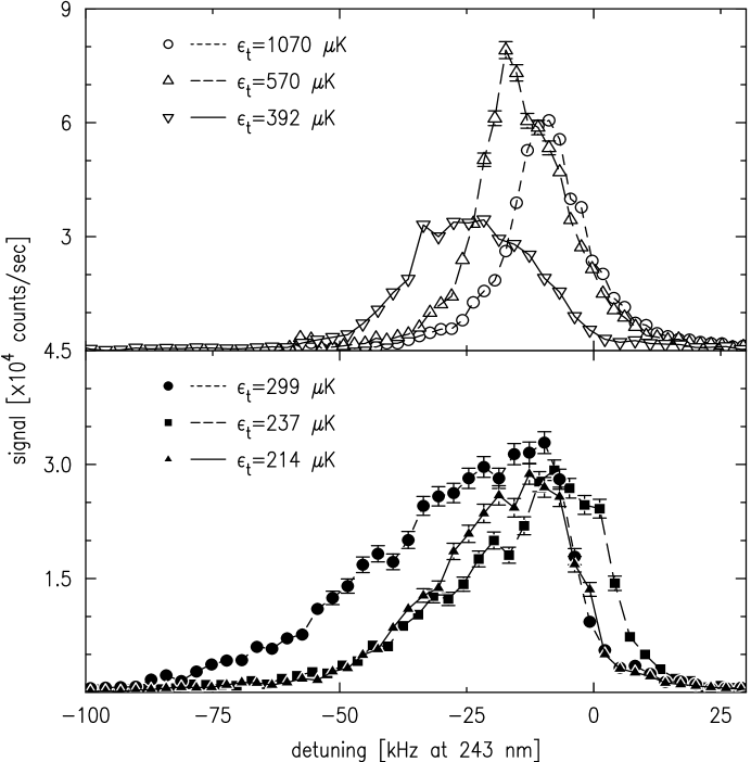
Figure 5-12: Doppler-free spectra of normal gas showing asymmetry in quantum degenerate regime. The spectra in the upper panel correspond to samples above quantum degeneracy; those in the lower panel are for samples that are degenerate. The trap shapes are identical, and the trap depths are indicated. Note the difference in vertical scale. The lines connecting the points are a guide to the eye. The error bars are statistical, and do not reflect systematic errors such as fluctuations in beam alignment and laser power.

Below the transition much of the spectral support is red-shifted to large detunings. These detunings, if simply interpreted as cold-collision frequency shift with the measured shift-to-density ratio $\chi_{m}$, correspond to sample densities a factor of two higher than expected for a degenerate Bose gas in equilibrium at a temperature which is reasonable for the trap. Note that $\chi_{m}$ was measured in samples far from quantum degeneracy. If $\chi$ were larger by a factor of two for the part of the cloud in the bottom of the trap where the effective chemical potential is small, then the asymmetric lineshape would make qualitative sense. The atoms in the highest density (red-shifted) part of the spectrum would tend to be shifted even further (because their $\chi$ is larger) than their low density counterparts. However, no quantitative theory has been formulated predicting that $\chi$ should vary for the normal gas as quantum degeneracy is approached.

5.6 Density Shift for Excitation out of the Condensate and the Normal Gas

A thorough treatment of the relation between $\chi_{c}$ and $\chi_{m}$ has been undertaken by Killian [13]. He concludes that $\chi_{c}=\chi_{m}/2$ because exchange effects should be present in the normal gas, but absent in a condensate. Here we discuss experimental evidence which suggests that perhaps $\chi_{c}=\chi_{m}$.

Time Evolution

As explained in section 5.4, the condensate is observed to persist for many seconds. Integration, over the lifetime of the condensate, of the rate of atom loss through dipolar decay in the condensate is very sensitive to $\chi_{c}$ because the loss rate is proportional to $n_{p}^{7/2}$; a factor of two difference in $\chi_{c}$ translates to a factor of 11 change in the loss rate. If we take $\chi_{c}=\chi_{m}/2$ then the number of atoms lost, $N_{c,lost}$ from equation 5.9, is as large as the total original population of the trap! The estimate here would be flawed if the trap parameters ($\alpha,\beta,\theta$) applicable to the condensate were somehow different from those for the thermal gas. This is unlikely, as noted in discussion of the trap shape in appendix G.

DS-DF Comparison

Doppler-sensitive excitation results in excited atoms moving at the recoil velocity $v_{recoil}\sim 3$ m/s. These motional states are very different from the low energy motional states inhabited during Doppler-free excitation. Furthermore, the high velocity of the recoiling atoms implies that motional coherence between the ground and excited states of the atom is very quickly lost during excitation, a situation conceivably different for DF excitation. Nevertheless, the condensate spectra obtained using the two different techniques are identical to within the (small) statistical uncertainty.

Spectroscopic Measurement of Condensate Fraction

The condensate fraction measured spectroscopically agrees well with the fraction one computes from the population in the condensate, assuming $\chi_{c}=\chi_{m}$. If $\chi_{c}=\chi_{m}/2$ then the calculated condensate fraction is $2^{5/2}\simeq 6$ times larger than indicated by the spectroscopic technique.

The possibility should be explored that $\chi=2\hbar(a_{2S-1S}-a_{1S-1S})/m$ (instead of $4\hbar(a_{2S-1S}-a_{1S-1S})/m$) for excitation out of the thermal gas. Then it would be easy to understand why $\chi_{c}=\chi_{m}$. Furthermore, the asymmetric spectra presented in section 5.5 could be understood if $\chi$ changed from the first to the second value in the normal gas near quantum degeneracy. If this were true all ambiguity would be relieved. Experiments designed to guarantee that the $1S$ and $2S$ atoms are distinguishable could conceivably provide insight into this issue. This possibility is addressed in section 6.3.5.

The Bose condensates reported in this chapter open possibilities for many new experiments. Some of these ideas are presented in the following chapter.

Chapter 6 Conclusion

6.1 Summary and Significance of this Work

We have created Bose-Einstein condensates of atomic hydrogen, culminating a long research effort. In the process we have confirmed that, as explained by Surkov et al. [32], the reduced dimensionality of the evaporation process was the crippling factor in previous efforts to reach this goal in our lab [29] and in Amsterdam [30]. Our condensates, while huge compared to other condensates, are only a small fraction of the total trap population, a prediction by Hijmans et al. [45] for spin-polarized hydrogen in equilibrium. We have this huge number of atoms in the trap because of the cryogenic loading technique we use, which can be scaled to arbitrarily large trap sizes (consistent with the scaling arguments in section 2.3.4). This cryogenic loading method has been generalized for arbitrary paramagnetic atoms and molecules by Doyle and coworkers [97, 98, 99, 100], and therefore it should be possible to create big condensates of arbitrary bosons. The high condensation flux we observe ($10^{9}$ atoms condensed per second for 10 s) should be useful in creating a bright atom laser. In addition, we have added another atom to the list of Bose-condensed species. In section 2.3 we explored many differences between the hydrogen system and the alkali metal gases that have been condensed so far. Finally, we have developed and applied spectroscopy as a new probe of condensates.

6.2 Improvements to the Apparatus

The experiments described in this thesis were frustrated by several factors. Changes in the apparatus could allow us to investigate several new areas.

One of the most straightforward improvements is to reduce the stray electric fields in the cell. Large fields reduce the lifetime of the $2S$ atomic state by Stark quenching; the lifetime in a static electric field $E$ (neglecting the natural lifetime) is [101]

$$\tau_{SQ}=\left(\frac{475~{}{\rm V/cm}}{E}\right)^{2}\;1.6~{}{\rm ns}.$$ (6.1)

In the current cell, with its non-conducting walls, static charges reduce the $2S$ lifetime to 0.1-1 ms, but in previous experiments in a metal cell [25] we have observed lifetimes on the order of the natural lifetime, $\tau_{0}=120~{}$ms. It should be possible to reduce stray fields by more than an order of magnitude by coating the inside of the plastic cell with a thin metallic film. Longer $2S$ lifetimes would allow us to address questions such as how interactions with the condensate affect the $2S$ lifetime. Also, low stray fields would allow atoms ejected from the condensate in an atomic beam to travel many centimeters toward the detector before decay (see section 6.3.3). Reduced stray fields would allow optical excitation to remain coherent for many milliseconds, allowing interesting studies of the excitation process. The large stray fields increase indirectly the background counts in our data: because of the short lifetime, fewer atoms can be accumulated in the $2S$ level before the detection pulse, and so more detection pulses must be used to accumulate the same signal. Each detection pulse increases the number of background counts. Reduction of stray fields would thus increase our sensitivity.

Another straightforward improvement is to reduce the heat load on the refrigerator caused by high power in the rf coils. The rf evaporation could then begin at higher sample temperatures, and more efficient cooling would undoubtedly result. More atoms in the condensate would increase the signal rates, and more detailed studies of the condensate would be possible. The heat load created by the rf coils appears to not be a consequence of the fields themselves, but rather of the system that conveys the power to the coils. If the coils were thermally anchored to the 4.2 K ⁴He bath the heating of the refrigerator should be dramatically reduced.

Better knowledge of the trap shape and laser alignment could allow more detailed studies of the influence of quantum degeneracy on the momentum distribution of the sample, as developed in section 6.3.2. As noted by Killian [13], better knowledge of trap and laser geometry would also allow more accurate measurements of $\chi$. We could better understand the sizes of the condensates we produce (recall how in section 5.4 the 20% error on $\chi_{m}$ translates into nearly a factor of two uncertainty in the number of condensate atoms lost during the lifetime of the condensate). The evidence for $\chi_{c}=\chi_{m}$ presented in section 5.6 could then be either bolstered or refuted, resulting in better understanding of the system.

The experiments probing the condensate, described in chapter 5, suffer from low signal rate. Straightforward improvements to the apparatus should allow at least a factor of 10 increase in detection solid angle, thus allowing studies at higher time resolution to be feasible. Condensate formation and feeding could be studied in more detail. The detection solid angle could be improved by moving the cold atoms into a short trap formed by small currents in thin coils. This small trap could be surrounded by Lyman-$\alpha$ detectors.

6.3 Suggestions for Experiments

The success of the experiments described in this thesis has fertilized thinking about many new experiments that could be done. In this section we discuss several of these ideas.

6.3.1 Creating Bigger Bose Condensates

Nearly any experiment is easier with a larger condensate, and so here we discuss strategies for putting more atoms into a hydrogen condensate.

First, more atoms could be initially loaded into the trap. We do not currently understand the loading process in detail. Investigations are underway to explore possibilities for loading more efficiently from the discharge. In addition to increasing the loading efficiency, one could also simply increase the physical volume of the trap by making it longer and of larger diameter. One should be able to load a factor of four more atoms by scaling up the apparatus using available technology.

The overall phase space compression efficiency exponent for cooling from loading conditions to BEC is $\gamma=-1.5$, which is small (see section A.2.3). Improvements to the cooling efficiency could be made using two strategies. The first is to commence rf evaporation earlier in the cooling cycle. The second is to increase the ratio of good collisions to bad collisions. It is probable that the admixture of an alkali “moderator” atom “M” in the sample could dramatically increase the effective collision rate without significantly increasing the dipolar decay rate [51]. Presumably the cross-section for H-M collisions would be much greater than the anomalously low H-H cross-section.

Finally, improvements could be made to the cooling procedure that do not require any changes to the apparatus. Instead of using the rf cooling paths shown in figure 5-4, the sample could first be compressed at constant trap depth, the depth being set by the highest rf frequency usable in the apparatus. Phase space compression would be accomplished at higher temperature, and thus more efficiently. After this compression the sample could be cooled to BEC at high density.

6.3.2 Probing the Velocity Distribution of the Normal Component of a Degenerate Gas

In section 5.3.2 we described the influence of quantum degeneracy on the velocity distribution of the normal gas. The expected spectrum is narrower and more cusp-shaped than for a classical gas at the same temperature. Here we consider an experiment designed to compare these spectra.

In order to ensure that the two samples (classical and quantum) being probed have the same temperature, we propose to use a single sample, but probe two parts of it. The inhomogeneous trapping potential serves to reduce the sample density (and thus the local chemical potential) in regions far from the deepest point in the trap. Classical behavior can be observed in a gas containing a condensate when the probe laser is translated a distance $\rho_{p}\gg{k_{B}}T/\alpha$ from the trap axis (for an IP trap with $T\geq\theta/{k_{B}}$). The beam diameter should be small compared to the translation distance, a condition that is easy to fulfill in an open trap (small $\alpha$).

The signal rate is dramatically reduced by the small densities far from the middle of the trap. In order to obtain the same signal rates as the present experiments (in which the high density central portion of the sample is probed), the detection efficiency must be increased by the ratio of the densities, $n(\rho=0)/n(\rho_{p})$. For trap B in table 5.2, and for $\rho_{p}=3{k_{B}}T/\alpha=160~{}\mu$m, the required improvement in detection efficiency is about

$$\frac{n(\rho=0)}{n(\rho_{p})}\simeq\frac{g_{3/2}(1)}{g_{3/2}(e^{-3})}\frac{\Upsilon_{1/2}(\eta,0)}{\Upsilon_{1/2}(\eta-3,-3)}\simeq 10^{2}.$$ (6.2)

Here we have used equation C.2 and figure C-1. A redesign of the apparatus for better optical access is required.

6.3.3 Creation of an Atom Laser

Atoms excited to the $2S$ state by co-propagating photons receive a momentum kick $p_{r}=2h/\lambda$ where $\lambda=243$ nm is the excitation wavelength. The atoms leave the excitation region with the recoil velocity $v_{r}=3.28$ m/s added vectorially to their initial velocity. In the normal gas there is a wide distribution of velocities, so only a tiny fraction are Doppler-shifted into resonance for a given detuning. In the condensate, however, the velocity distribution is very narrow, and one might expect to interact optically with all the condensate atoms at the same laser tuning. Atoms excited out of the (coherent) condensate by a laser beam with a long coherence time should constitute a coherent atomic beam. The divergence of this beam of atoms should be diffraction limited by the size of the excitation region. Such a scheme has been demonstrated by Kozuma et al. [96] using Raman pulses.

Unfortunately, several complications arise. First, the condensate spectrum is broadened by the cold-collision frequency shifts arising from the high and inhomogeneous condensate density. Since these shifts are much greater than the laser linewidth, the laser only interacts with a small fraction of the condensate for a given detuning. (One can imagine efficient methods of broadening the laser linewidth to match the condensate linewidth [102], resulting in excitation of all the condensate atoms, but this broadening would write decoherence onto the ejected atoms.) Since the optical radiation only excites atoms from regions of a given density (corresponding to the detuning), the excitation region can be quite small, and the divergence of the beam is enlarged. For example, atoms excited by a laser beam of linewidth 2 kHz that is tuned to the peak condensate density will come from a region of diameter on the order of $\omega_{exc}=1~{}\mu$m. The resulting divergence angle is $h/p_{r}\pi\omega_{exc}=4\times 10^{-2}$ [103]. The situation is more complicated when the laser is detuned to interact with atoms in regions of intermediate density. Here the excitation occurs on a shell; interesting diffraction effects should occur.

As the $2S$ atoms propagate with recoil velocity $v_{r}$, the potential surface they experience is strongly perturbed by the strong attractive mean field potential created by the high condensate density. The depth of this potential for the peak condensate densities listed in table 5.2 is on the order of $50~{}\mu$K. The depth is small compared to the $650~{}\mu$K of recoil kinetic energy, so the atom has enough energy to leave the condensate. However, the depth is much larger than the energy in the radial coordinates, $\mu/{k_{B}}=2~{}\mu$K. One expects focusing effects as the recoiling atoms leave the condensate.

The $1S$-$2S$ excitation process does not effect the hyperfine state of the atom; the recoiling atoms are still in the $d$-state, and are trapped. As the atoms move toward the magnetic barrier that forms the end of the trap they slow down. Dephasing also occurs because the integrated action for slightly different atomic trajectories quickly becomes quite different in the mountainous potential surface the atoms explore as they leave the trapping region. In order to circumvent these problems of slowing and dephasing we propose to flatten the potential surface: we put the atoms in a magnetic field insensitive state by driving the $d$-$a$ transition for the $2S$ atoms. The transition can be driven selectively for only the $2S$ atoms because the hyperfine splitting of the $2S$ state is $2^{3}=8$ times smaller than the $1S$ hyperfine splitting of 1420 MHz. One might be concerned that the rf field would drive $d$-$c$ state transitions in the cold cloud of $1S$ atoms, and thus change the effective trap depth. This does not occur because the frequency is too large (178 MHz corresponds to a trap depth of 8.5 mK). The $a$-state $2S$ atoms are free to fall out of the trapping region. In the current apparatus the atoms can fall a height $h=20$ cm before hitting a window. This should take a time $\tau_{fall}=(-v_{r}/g)(1-\sqrt{1+2gh/v_{r}^{2}})=56$ ms for atoms with downward directed recoil velocity, and $\tau_{fall}=(v_{r}/g)(1+\sqrt{1+2gh/v_{r}^{2}})=790$ ms for those with upward directed recoil velocity. Here $g$ is the acceleration of gravity. We do not expect to detect the atoms launched upward because the natural lifetime (120 ms) is too short, and because, in the current apparatus, the atoms will hit a surface before reaching the peak of their 55 cm high trajectory.

Detection of the atomic beam could be accomplished by quenching the atoms with an applied electric field pulse when the atoms are at the bottom of the cell near the detector. To estimate the signal size, we compare to the signal obtained when the atoms are not allowed to move very far before detection, the experimental procedure for figure 5-5. We expect a reduction in the number of fluorescing atoms by $e^{-\tau_{fall}/\tau_{0}}\simeq 0.63$ because of decay during the transit time $\tau_{fall}$. We expect a factor of two further reduction because only $1/2$ the atoms have downward-directed recoil velocity. We expect an increase in signal because the detection solid angle is greater near the bottom of the cell. With the current cell design we should be able to achieve a factor of seven increase in detection efficiency, but with straightforward extensions of the cell closer to the detector this factor could be another factor of ten larger. Neglecting this improvement, we expect the atoms in the atomic beam to yield about the same signal size as observed in figure 5-5. The experiment is thus feasible in a cell identical to the current one, but a conductive coating to reduce stray electric fields is essential.

In addition to observing an atomic beam ejected from the sample, another interesting experiment would be a study of collisional quenching of the $2S$ atoms as they move through the high density condensate. One might expect collisional de-excitation to occur on a time scale comparable to the characteristic collision time: $\tau_{col}=1/n_{p}\sigma_{2S-1S}v_{recoil}\simeq 700~{}\mu$s. A brief study indicated no collisional quenching on the sub-millisecond time scale, but the study should be repeated for longer times. Reduction of the stray fields would allow this.

6.3.4 Measuring the Condensate Density through Dipolar Decay

In the experiments described in chapter 5 the condensate density was measured spectroscopically, but confusion arises around a factor of two in the conversion constant $\chi_{c}$ that relates frequency shift to sample density. We propose an independent measure of condensate density which should resolve the ambiguity. The proposed measurement exploits two-body dipolar decay, which proceeds at a well known rate in the condensate [44]. If the condensate density distribution is well approximated by the Thomas-Fermi profile in equation 2.13, then the characteristic loss rate is given by equation 2.15. Using equation 2.14 we find that the peak shift (frequency shift of maximally shifted part of the spectrum) should decay in time as

$$\Delta_{p}(t)=\frac{\Delta_{p,0}}{1+\frac{4g\Delta_{p,0}}{35\chi_{c}}t}$$ (6.3)

where $\Delta_{p,0}$ is the initial peak shift. The only free parameters used to fit this equation to measured data would be $\Delta_{p,0}$ and $\chi_{c}$. The factor of two ambiguity in $\chi_{c}$ should be easy to resolve. If the Thomas-Fermi density distribution is a poor approximation, then the factor $4/35$ should be different. The quality of the fit of the Thomas-Fermi lineshape to the data in figures 5-5, 5-6, 5-9, and 5-10 indicates that this approximation is reasonable.

To measure the condensate decay time cleanly, we require that the condensate is not being replenished by the normal gas. The most straightforward way to accomplish this is a complete removal of the normal gas by rf ejection. The trap depth would be quickly swept down to the edge of the condensate, using high rf power to efficiently outcouple all the normal atoms. DF or DS spectroscopy of the condensate would then probe the time evolution of the peak shift, $\Delta_{p}(t)$.

Since the lifetime of the condensate would be short, there would not be much signal accumulation time. The detection efficiency in the current apparatus is too low, but a factor of six improvement should make this experiment feasible (a factor of six can be obtained by replacing the Lyman-$\alpha$ filter over the MCP with a window). Currently, sufficient signal can be obtained by summing 0.8 s sweeps from several identically prepared samples. A factor of six improvement would allow the sweeps to be shortened to 0.13 s, short compared to the decay time $35\chi_{c}/4g\Delta_{p,0}\simeq 1$ s expected for $\chi_{c}=\chi_{m}/2$ and $\Delta_{p,0}\sim 600$ kHz.

6.3.5 Exchange Effects in Cold-Collision Frequency Shift

In section 5.6 we proposed that perhaps $\chi_{c}=\chi_{m}$, which would make sense if $\chi_{m}$ did not include exchange effects for some reason. This could be tested by measuring the cold-collision frequency shift in the classical regime for atoms that are known to be distinguishable. To ensure distinguishability, the atoms could be put into different hyperfine states, $c$ and $d$. A $c$-state atom interacting with a $d$-state atom should follow an interaction potential that is very similar to the identical particle case, but the mean-field interaction energy would be smaller by a factor of two because the atoms are distinguishable and exchange effects are absent. One expects two peaks in the DF spectrum: one from collisions between identical particles, which is shifted twice as much as the other, which is from collisions between distinguishable particles. If the observed spectrum contains only a single peak, then we conclude that the atoms are distinguishable in all collision processes. In that case we expect $\chi_{c}=\chi_{m}$.

We propose to do this experiment in a very deep trap (${\epsilon_{t}}/{k_{B}}\gg(\mu_{B}/{k_{B}})506~{}{\rm G}=34$ mK) so that the $c$-state atoms will be confined (see figure 1-1). We propose to use a sample typical of what exists immediately after loading the trap ($T=40$ mK, $n_{0}=2\times 10^{13}~{}{\rm cm^{-3}}$). If half the atoms are transferred from the $d$ to the $c$ state, the expected decay time of the $c$-state atoms is $\tau\simeq 2$ s. The dominant terms in the loss rate are $G_{cc\rightarrow aa}=1.4\times 10^{-13}$, $G_{cc\rightarrow bd}=7\times 10^{-14}$, and $G_{cc\rightarrow ac}=6\times 10^{-14}~{}{\rm cm^{3}/s}$ for fields around 600 G [104], which corresponds to the thermal energy. We must measure the DF spectrum quickly compared to this time $\tau$ to observe how the spectrum changes.

Time-of-flight broadening would be significant in this spectrum, on the 40 kHz level for the current laser beam waist (100 $\mu$m diameter). This is large compared to the expected cold-collision frequency shifts of 2 and 4 kHz. To reduce the broadening, the beam diameter could be expanded by a factor of ten. The excitation rate (proportional to the square of the radiation intensity) would drop by $10^{4}$, but the interaction volume would increase by $10^{2}$ (the sample diameter is larger than the beam diameter). The linewidth would narrow by a factor of ten because of the increased interaction time, and so the overall signal rate would drop by only a factor of ten. Samples can be created every two minutes and systematics are easy to control, so it would be straightforward to accumulate signal.

6.3.6 Measuring $a_{1S-1S}$

The ground state $s$-wave scattering length has been calculated to the level of $10^{-2}$ [40], but has not been measured nearly as well. One could use the interaction energy $U_{0}n_{p}=4\pi\hbar^{2}an_{p}/m$ in the condensate to measure $a$, given the peak density $n_{p}$. We propose to measure the chemical potential $\mu$ directly in an experiment similar to the measurement of $\chi_{c}$ in section 6.3.4. Using $\mu=U_{0}n_{p}$ we obtain $a=\mu m/4\pi\hbar^{2}n_{p}$. To get $\mu$ we measure the difference between the potential energies at the center ($\theta$) and edge ($\varepsilon_{e}$) of the condensate. We measure $\theta$ by sweeping the rf frequency upward until atoms begin to fall out of the trap, as described in section 4.2.4. We measure $\varepsilon_{e}$ in a series of measurements of the sample density; the normal atoms are removed by sweeping the rf frequency down to some ending frequency $f_{end}$, which is varied. For $f_{end}$ slightly larger than $\varepsilon_{e}/h$ the density measurements should give identical results. But for $f_{end}<\varepsilon_{e}/h$ the condensate is depleted, and the measured density decreases.

A measurement of $a$ to the 10% level seems feasible. Consider trap B and a peak condensate density $n_{p}=3\times 10^{15}~{}{\rm cm^{-3}}$. The bias field $\theta$ must not drift more than 1 mG between measurement of $\theta$ and $\varepsilon_{e}$; this stability should be possible. To measure $\varepsilon_{e}$ we vary $f_{end}$ and look for changes in the maximum frequency shift, as described above. Since the maximum frequency shift scales linearly with the chemical potential, we must measure $\Delta_{p,0}$ to better than 10%. This should be possible with the factor of six detection efficiency improvement outlined above. Many spectra would be obtained as the condensate decays, and so a group of many data points would be fit to the two parameters in equation 6.3. Precision of 10% seems feasible.

6.3.7 Dynamics of $2S$ atoms in $1S$ condensate

As described in section 5.3.1 and in the thesis of Killian [13], condensate atoms excited to the $2S$ state are confined radially by the deep interaction potential created by the large condensate density. The motional eigenstates in the $2S$ potential are rather different from the $1S$ eigenfunction, the condensate wavefunction. We therefore expect the $2S$ atoms to exist in superpositions of several of these excited state eigenfunctions, and to thus oscillate across the condensate.

The initial position of the $2S$ atoms is tuned by the detuning of the excitation radiation field. The position after some delay time $\tau$ could be measured using Balmer-$\alpha$ absorption imaging. One expects breathing modes. Coherence effects in the excitation process could be explored with this technique.

6.4 Outlook

The studies of Bose condensed hydrogen presented here constitute simply the appetizer in the feast of experiments to be carried out. Once ambiguities about $\chi_{c}$ are straightened out and the fascinating asymmetric lines in section 5.5 are understood, the creation of the high-flux coherent atomic seems to be the next step. The beautiful atom laser experiments of Mewes et al. [105], Kozuma et al. [96], and Anderson and Kasevich [11] should provide solid stepping stones.

Appendix A Theory of Trapped Classical Gas

In this appendix we present the statistical mechanical treatment of a trapped ideal gas, consider decay of the sample through relaxation of the spin-polarization, and calculate the effects of evaporation. The appendix exists to familiarize the reader with concepts and scaling laws useful for hydrogen trapping and cooling experiments. Simple relations describe samples trapped in deep potentials. Here we address the effects of the finite trap depth, following the work of Luiten et al. [26]. We find that the truncation corrections are only important for shallow traps.

A.1 Ideal Gas

We begin our discussion by describing a trapped ideal gas in the classical regime. “Trapped” implies confinement by an inhomogeneous potential with a depth significantly greater than the characteristic energy of the gas particles. “Ideal” means that collisions among the atoms, although crucial for maintaining thermal equilibrium, are not included in the Hamiltonian. The interaction energy for the densities studied in this thesis will turn out to be very small compared to the thermal energy, except in the case of when a condensate, as described in section 2.2.2. “Classical” means that the gas is far from quantum degeneracy, and the Maxwell-Boltzmann distribution adequately describes the correct quantum distribution. These approximations are appropriate for the trapped hydrogen gas studied in this thesis as it is cooled from the initial temperature of about 40 mK to near the onset of quantum degeneracy around $50~{}\mu$K.

In sections A.1.1 and A.1.2 we describe the occupation function for the gas and the density of states functions for traps of experimental interest. In section A.1.3 these concepts are employed to calculate various thermodynamic properties. In section A.1.4 we consider trap losses arising from decay of the spin-polarization of the trapped gas. Collisions and evaporative cooling are the topics of section A.2.

A.1.1 Occupation Function

We assume that the gas is well described by the Maxwell-Boltzmann distribution, except that the energy distribution is truncated at some trap depth energy ${\epsilon_{t}}$. The gas is said to be quasi-thermal. This is a reasonable assumption if two conditions hold [26]. First, the elastic collision rate must be high enough to redistribute particle energies quickly compared to the rate at which processes occur which would take the gas out of equilibrium, such as changes in the trap shape or depth. This is called the “sufficient ergodicity” condition. (Elastic collisions are discussed in section A.2 below.) Second, particles with energies greater than the trap depth must be removed promptly compared to the rate at which they are promoted to the energetic states. Situations in which this condition is not satisfied have been discussed in section 2.1.

The phase space occupation function, $f(\epsilon)$, is the number of particles per unit volume of phase space in a region of phase space with total energy $\epsilon={\cal H}({\bf p},{\bf r})$. (${\cal H}$ is the Hamiltonian of the particle). We postulate an occupation function $f(\epsilon)$ that is the Boltzmann factor [33] below the trap depth, and zero above:

$$f(\epsilon)=\left\{\begin{array}[]{lll}n_{0}\Lambda^{3}e^{-\epsilon/{k_{B}}T}&;&\epsilon\leq{\epsilon_{t}}\\ 0&;&\epsilon>{\epsilon_{t}}\end{array}\right.$$ (A.1)

where $\Lambda\equiv h/\sqrt{2\pi m{k_{B}}T}$ is the thermal de Broglie wavelength and $n_{0}$ is a reference density; the normalization is the total number of trapped atoms. Evidence supporting this postulate was obtained by numerical integration of the Boltzmann transport equation [26]. The occupation function of a simulated gas, described initially by $f(\epsilon)=$const. below threshold ${\epsilon_{t}}$ and zero above, was observed to transform to the Boltzmann form in equation A.1 in a few characteristic collision times. The trapped gas is described by two parameters, $T$ and $n_{0}$, which correspond to sample temperature and maximum sample density in an infinitely deep trap [26]. For finite trap depths, temperature is poorly defined because the distribution is truncated, and $n_{0}$ is larger than the actual maximum sample density, as discussed in section A-1.

A.1.2 Density of States

A useful concept is the density of states, the volume of parameter space corresponding to the fulfillment of some condition. We use two density of states functions. The “total energy density of states” function, $\rho(\epsilon)$, is the differential volume of phase space corresponding to a total particle energy $\epsilon$. (The number of particles $N(\epsilon)d\epsilon$ within an energy $d\epsilon$ of $\epsilon$ is the occupation per unit volume multiplied by the volume, $N(\epsilon)d\epsilon=f(\epsilon)\rho(\epsilon)d\epsilon$.) The “potential energy density of states” function, $\varrho(\varepsilon)$, is the differential volume of real space with potential energy $\varepsilon$. In this thesis $\varepsilon$ will always denote a potential energy, and $\epsilon$ will always denote a total energy. Likewise, $\varrho(\varepsilon)$ will always be a potential energy density of states, and $\rho(\epsilon)$ will always be a total energy density of states.

The total energy density of states function is

$$\rho(\epsilon)=\frac{1}{h^{3}}\int d^{3}{\bf p}\,d^{3}{\bf r}\,\delta({\cal H}({\bf p},{\bf r})-\epsilon)$$ (A.2)

where the Hamiltonian is ${\cal H}=p^{2}/2m+V({\bf r})$, and $V({\bf r})$ describes the trap potential. Using $\rho(\epsilon)$, integrals over phase space of a function $F({\cal H}({\bf r},{\bf p}))$, which depends only on the total particle energy, can be converted from the six dimensional integral $\int d^{3}{\bf r}d^{3}{\bf p}F({\cal H}({\bf r},{\bf p}))$ to a one dimensional integral over energy $\int d\epsilon\rho(\epsilon)F(\epsilon)$.

The potential energy density of states function is

$$\varrho(\varepsilon)\equiv\int d^{3}{\bf r}\,\delta(V({\bf r})-\varepsilon)$$ (A.3)

The trap shapes, $V({\bf r})$, in our experiments are well approximated by either of two model potentials. Both potentials are cylindrically symmetric, and we use $z$ for the axial coordinate and $\rho$ for the radial coordinate. The aspect ratio of the confined clouds (length/diameter) is typically between 10 and 400. The “quadrupole trap with hard wall ends” [106, 17] approximates traps used at higher temperatures ($T\geq 1$ mK), and was treated by Doyle [17]. The second model trap shape is often called the “Ioffe-Pritchard” [31, 26] (labeled “IP”). It corresponds to the potential we use at the lowest temperatures and has the form

$$V_{IP}(\rho,z)=\sqrt{(\alpha\rho)^{2}+(\beta z^{2}+\theta)^{2}}-\theta$$ (A.4)

with radial potential energy gradient $\alpha$, axial potential energy curvature $2\beta$ (units of energy/distance²), and bias potential energy $\theta$. The potential energy density of states for this trap is

$$\varrho(\varepsilon)=\frac{4\pi}{\alpha^{2}\sqrt{\beta}}\;\sqrt{\varepsilon}\>(\varepsilon+\theta).$$ (A.5)

We define the prefactor ${\cal A}_{IP}=4\pi/\alpha^{2}\sqrt{\beta}$, with units (volume)(energy)^-5/2. The total energy density of states for this trap is

$$\rho(\epsilon)=\frac{(2\pi m)^{3/2}}{h^{3}}\frac{\pi^{3/2}}{2\alpha^{2}\sqrt{\beta}}\;\epsilon^{2}(\epsilon+2\theta).$$ (A.6)

We define the prefactor $A_{IP}=\pi^{2}m^{3/2}{\cal A}_{IP}/h^{3}2^{3/2}$, which has units of (energy)^-4.

A.1.3 Properties of the Gas

Properties of the gas, such as population, energy, and density, may be calculated using the phase space occupation function and density of states functions [33]. The number of trapped atoms, $N$, is

$$N = \int_{0}^{{\epsilon_{t}}}d\epsilon\,f(\epsilon)\rho(\epsilon)$$ (A.7)

$$= n_{0}\Lambda^{3}{{\cal Z}}$$

where the single particle partition function is

$${{\cal Z}}=\int_{0}^{{\epsilon_{t}}}d\epsilon\;\rho(\epsilon)\exp(-\epsilon/{k_{B}}T)$$ (A.8)

The $N$-particle partition function for a non-interacting classical gas is ${{\cal Z}}_{N}={{\cal Z}}^{N}/N!$.

For a power law density of states given as $\rho(\epsilon)=\rho_{0}\>\epsilon^{\delta+3/2}$ we obtain

$${{\cal Z}}={{\cal Z}_{\infty}}P(\delta+5/2,\eta)$$ (A.9)

where $\eta\equiv\epsilon_{t}/{k_{B}}T$ is a dimensionless measure of the trap depth (typically $4<\eta<10$) and

$${{\cal Z}_{\infty}}\equiv\rho_{0}({k_{B}}T)^{\delta+5/2}\Gamma(\delta+5/2)$$ (A.10)

is the partition function for an infinitely deep trap. The truncation correction factor $P(q,\eta)$ is defined in equation A.12.

The partition function for the IP potential is

$${\cal Z}_{IP}=\frac{({k_{B}}T)^{5/2}3\pi^{3/2}}{\Lambda^{3}\alpha^{2}\sqrt{\beta}}\left(P(4,\eta)+\frac{2\phi}{3}P(3,\eta)\right)$$ (A.11)

where $\phi\equiv\theta/{k_{B}}T$ is a dimensionless measure of the trap bias energy and $\eta\equiv{\epsilon_{t}}/{k_{B}}T$ is a dimensionless measure of the trap depth. We have introduced the function $P(q,\eta)$, which is a correction factor for the finite trap depth [26]. It is related to the incomplete gamma function $\Gamma(q,\eta)\equiv\int_{\eta}^{\infty}t^{q-1}e^{-t}dt$ by

$$P(q,\eta) \equiv \frac{1}{\Gamma(q)}\int_{0}^{\eta}t^{q-1}e^{-t}dt$$ (A.12)

$$= \frac{\Gamma(q)-\Gamma(q,\eta)}{\Gamma(q)}$$

For large $\eta$ the correction is negligible, and $P(q,\eta)=1$. The behavior of $P(q,\eta)$ is shown in figure A-1 for various values of $q$.

Figure A-1: The behavior of the truncation correction factor $P(q,\eta)$, plotted for various exponents $q$. The values $q=3$ and $q=4$ are used in finding the population of the IP trap. The value $q=3$ (heavy solid line) is for a harmonic trap.

The parameter $q$ describes the energy exponents appearing in the trapping potential. As stated in equation A.11, the values $q=3$ and $q=4$ are of interest for the IP trap. Note that for $\eta\geq 7$ there is only a small deviation from the infinitely deep trap (corresponding to $\eta\rightarrow\infty$) for the exponents $\delta$ of interest in this thesis.

The effective volume of the trap is

$${V_{eff}}\equiv N/n_{0}={{\cal Z}}\Lambda^{3}.$$ (A.13)

The energy of the trapped gas is

$$E = \int_{0}^{{\epsilon_{t}}}d\epsilon\,\epsilon\rho(\epsilon)f(\epsilon)$$ (A.14)

For the IP trap

$$E_{IP}=4{k_{B}}TN_{IP}\frac{P(5,\eta)+\frac{\phi}{2}P(4,\eta)}{P(4,\eta)+\frac{2\phi}{3}P(3,\eta)}.$$ (A.15)

This result will be used in section A.2.2. The average energy per particle is $\overline{E}=E/N$.

The density at a position ${\bf r}$ (with potential energy $\varepsilon=V({\bf r})$) may be obtained as follows. Using the phase space occupation function

$$f({\bf r},{\bf p})=n_{0}\Lambda^{3}\exp\left(-\frac{V({\bf r})+p^{2}/2m}{{k_{B}}T}\right)$$ (A.16)

we integrate over trapped momentum states to obtain [26]

$$n({\bf r})=n_{0}e^{-V({\bf r})/{k_{B}}T}\left({\rm erf}(t)-2te^{-t^{2}}/\sqrt{\pi}\right)$$ (A.17)

where $t=\sqrt{({\epsilon_{t}}-V({\bf r}))/{k_{B}}T}$ and ${\rm erf}(t)\equiv 2\int_{0}^{t}e^{-s^{2}}ds/\sqrt{\pi}$ is the error function. Note that for an infinitely deep trap

$$n({\bf r})=n_{\infty}({\bf r})\equiv n_{0}e^{-V({\bf r})/{k_{B}}T}.$$ (A.18)

The ratio of the density $n({\bf r})$ in a region of potential energy $\varepsilon=V({\bf r})$ to the density $n_{\infty}(0)$ at the bottom of an infinitely deep trap is shown in figure A-2. We see that, for $\eta>6$, truncation does not significantly effect the density near the bottom of the trap where $\epsilon$ is less than a few ${k_{B}}T$.

Figure A-2: The effect of truncation of the energy distribution on the density in the trap in a region of potential energy $\varepsilon$, plotted for various trap depths $\eta={\epsilon_{t}}/{k_{B}}T$.

A.1.4 Dipolar Decay

In this section we calculate the effect of spin relaxation on the population and energy of the trapped gas. Spin relaxation is the dominant loss process in our trap. In this analysis we properly treat truncation of the energy distribution, following Luiten et al. [26].

Dipolar spin relaxation is a process in which the magnetic dipoles of two atoms interact, leading to a spin flip of one or both atoms [57]. If one of the interacting atoms makes a transition from the trapped $d$-state to the $a$ state (see figure 1-1), the hyperfine energy, corresponding to 68 mK, is released and both atoms are ejected from the trap. An atom that makes a transition to the $c$-state is weakly trapped in the radial direction, but is pulled by gravity out of the trap through the weak fields along the trap axis. An atom that makes a transition to the high field seeking $b$ state is expelled from the trap. The rate constant for loss from the trapped $d$ state has been calculated [104] and measured to the 20% level [107, 23]. The calculated rate constant for loss from the $d$ state through all channels at low temperatures is

$$g = 2(G_{dd\rightarrow aa}+G_{dd\rightarrow ad}+G_{dd\rightarrow ac}+G_{dd\rightarrow cc})+G_{dd\rightarrow cd}$$ (A.19)

$$= 1.2\times 10^{-15}~{}{\rm cm}^{3}~{}{\rm s}^{-1},$$

where $G_{\sigma\lambda\rightarrow\phi\psi}$ is the event rate for the process in which two atoms in the $\sigma$ and $\lambda$ states make transitions to the $\phi$ and $\psi$ states. The rate depends very weakly on magnetic field, but we ignore the dependence for the low temperature experiments which are the focus of this thesis.

The dipolar decay rate from a region of density $n$ is $\dot{n}=-gn^{2}$. Consequently, loss occurs most rapidly from regions of high density near the bottom of the trap. The rate at which atoms are lost from the trap through dipolar decay is

$$\dot{N}_{2}=-g\int_{0}^{{\epsilon_{t}}}d\varepsilon\,\varrho(\varepsilon)n^{2}(\varepsilon)$$ (A.20)

where $n(\varepsilon)$ is the gas density in regions with potential energy $\varepsilon$. An effective volume for dipolar decay, $V_{2}$, is defined by

$$\dot{N}_{2}=-gn_{0}^{2}\>V_{2}=-gn_{0}N\left(\frac{V_{2}}{V_{eff}}\right)$$ (A.21)

The ratio $V_{2}/V_{eff}$ for the IP trap is plotted in figure A-3. The volume for dipolar decay is smaller than the effective volume because dipolar decay occurs preferentially in regions of highest density, which are restricted to the bottom of the trap.

Figure A-3: The volume for dipolar decay compared to the effective volume, plotted for various bias fields $\phi=\theta/{k_{B}}T$. The difference between large $\phi$ (harmonic) and small $\phi$ (linear radial confinement) arises because in the harmonic trap the density distribution is flatter in the middle. For a box potential the density distribution is completely flat, and the two volumes are identical.

Since relaxation occurs predominantly near the bottom of the trap, the escaping atoms typically have less energy than the sample average energy per particle, $\overline{E}$. Dipolar decay is thus a heating mechanism. The energy loss rate is the integral over the trap of the local loss rate multiplied by the local average of the total energy per particle:

$$\dot{E}_{2}=-g\int_{0}^{{\epsilon_{t}}}d\varepsilon\,\varrho(\varepsilon)n^{2}(\varepsilon)\left(\varepsilon+\overline{K}(\varepsilon)\right).$$ (A.22)

The average kinetic energy per particle is $\overline{K}=3{k_{B}}T/2$ in an untruncated Maxwell-Boltzmann distribution of velocities, but here we include the finite trap depth in $\overline{K}$. We calculate the average kinetic energy per particle for particles with potential energy $\varepsilon$ in a trap of depth ${\epsilon_{t}}$:

$$\overline{K}(\varepsilon) = \frac{\displaystyle\int_{0}^{\sqrt{2m({\epsilon_{t}}-\varepsilon)}}d^{3}p\,\frac{p^{2}}{2m}e^{-p^{2}/2m{k_{B}}T}}{\displaystyle\int_{0}^{\sqrt{2m({\epsilon_{t}}-\varepsilon)}}d^{3}p\,e^{-p^{2}/2m{k_{B}}T}}$$ (A.23)

$$= {k_{B}}T\frac{6t+4t^{3}-3s}{4t-2s}$$

where $s=\sqrt{\pi}{\rm erf}(t)\exp(t^{2})$ and $t=\sqrt{({\epsilon_{t}}-\varepsilon)/{k_{B}}T}$. Figure A-4 shows the behavior of $\overline{K}$.

Figure A-4: The mean kinetic energy of atoms in a region of given potential energy, plotted for samples in traps of various depths. The trap appears shallower for atoms at higher potential energies.

The average energy carried away per atom is $C_{2}{k_{B}}T\equiv\dot{E}_{2}/\dot{N}_{2}$. This is plotted in figure A-5 for the IP trap, for various values of $\phi$. We see that for $\eta\geq 6$ we can reasonably ignore truncation effects.

Figure A-5: The average total energy per atom that is lost from a Ioffe-Pritchard trap through dipolar relaxation, in units of ${k_{B}}T$. The parameter $\phi\equiv\theta/{k_{B}}T$ is the strength of the bias field, and $\eta\equiv\epsilon_{t}/{k_{B}}T$ is the trap depth. We see that we can ignore truncation effects for $\eta\geq 6$. For the harmonic trap (large $\phi$) the particles have less potential energy because the potential is quadratic; in the linear radial potential (small $\phi$) there is more potential energy per particle.

A.2 Collisions and Evaporative Cooling

So far we have not addressed elastic collisions, but they play a crucial role in the dynamics of the trapped gas. In this section we examine we examine the role of collisions in maintaining thermal equilibrium and in evaporatively cooling the sample. We calculate the equilibrium temperature of the gas. And we conclude the section with a discussion of an impediment to efficient evaporative cooling, the impediment that prevented the creation of BEC in hydrogen before this work.

Only low energy collisions occur in our cold samples, so the elastic scattering process is described by quantum mechanical $s$-wave scattering theory [108, 27]. The result of this theory is that elastic interactions are parameterized by a single quantity, the $s$-wave scattering length $a$. The cross section for collisions between identical particles is $\sigma=8\pi a^{2}$. In a gas of density $n$ and mean particle speed $\bar{v}=\sqrt{8{k_{B}}T/\pi m}$, the collision rate is $\Gamma_{col}(n)=n\sigma\bar{v}\sqrt{2}$. The collision rate determines the time scale for energy redistribution in the gas.

A sample in a trap of finite depth is never in complete equilibrium since collisions constantly tend to populate that portion of the equilibrium energy distribution which lies above the trap depth. The removal of these energetic atoms is called evaporation. Its use as a cooling mechanism for a trapped atomic gas was first proposed by Hess [106] and was first demonstrated in the MIT spin-polarized hydrogen group [109]. Evaporation occurs when a collision of two atoms transfers enough energy to one atom that it may escape the trap. This atom leaves the trap with an energy $\epsilon>{\epsilon_{t}}$, much greater than the average energy per atom in the sample, $\overline{E}$. The average energy per remaining particle is lower, and after rethermalization of the trapped gas, the temperature is lower. Cooling has occurred. Note that rethermalization is given a headstart by the preferential evaporation of atoms from the upper end of the energy distribution, closer in energy to the trap depth, ${\epsilon_{t}}$, as described in appendix B.

A.2.1 Evaporative Cooling Rate

The evaporative cooling rate for a sample described by a truncated Boltzmann occupation function has been calculated by Luiten et al. [26] using the Boltzmann transport equation. We quote their results here.

The particle loss rate due to evaporation is

$$\dot{N}_{evap}=-n_{0}^{2}\,\sigma\,\bar{v}\,V_{evap}=-N\>\frac{\Gamma_{col}(n_{0})}{\sqrt{2}}\>\frac{V_{evap}}{V_{eff}},$$ (A.24)

a product of the total population, a characteristic collision rate, and the fraction of collisions which produce an atom with enough energy to escape. The ratio $V_{evap}/V_{eff}$ for an IP trap is plotted in figure A-6 for various $\phi=\theta/{k_{B}}T$ (we use equation 43a from [26]).

Figure A-6: The quantity $V_{evap}/V_{eff}$ for an IP trap as a function of $\eta$, plotted for various bias fields $\phi=\theta/{k_{B}}T$. The inset shows $V_{evap}e^{\eta}$, which becomes linear in $\eta$ for large $\eta$. This linear relation is useful when estimating evaporation rates.

The energy loss rate due to evaporation is given by equation 40 in [26]:

$$\dot{E}_{evap}=\dot{N}_{evap}{k_{B}}T\left\{\eta+1-X_{evap}/V_{evap}\right\}$$ (A.25)

where $X_{evap}$ is a truncation correction factor. Figure A-7 shows the behavior of $X_{evap}/V_{evap}$ for the IP trap (we use equation 43b from [26]).

Figure A-7: The quantity $X_{evap}/V_{evap}$ for an IP trap as a function of $\eta={\epsilon_{t}}/{k_{B}}T$, plotted for various bias fields $\phi=\theta/{k_{B}}T$. The volume $X_{evap}$ is a small contribution to the evaporation volumes for $\eta\geq 6$

For large $\eta$, the quantity in curly braces in equation A.25 is nearly $\eta+1$.

A.2.2 Equilibrium Temperature

The temperature of the trapped gas is set by a competition between heating due to dipolar relaxation and cooling due to evaporation. The sample is in dynamic equilibrium when the temperature is no longer changing, meaning that the average energy per particle is stationary. Setting $d(E/N)/dt=0$ dictates that

$$\frac{E}{N}=\frac{\dot{E}}{\dot{N}}=\frac{\dot{E}_{evap}+\dot{E}_{2}}{\dot{N}_{evap}+\dot{N}_{2}}$$ (A.26)

If the temperature drops below equilibrium, the evaporation rate drops exponentially. In addition, the effective volume decreases, the density increases, and the heating rate due to dipolar decay increases. On the other hand, if the temperature increases above equilibrium, the heating rate decreases and the evaporative cooling rate increases. A dynamic equilibrium is thus maintained.

The equilibrium temperature is found by numerically solving equation A.26. For notational simplicity we define the factor $B$ which indicates whether the IP trap is primarily linear or harmonic in the radial direction,

$$B(\eta,\phi)\equiv\frac{P(5,\eta)+\phi P(4,\eta)/2}{P(4,\eta)+2\phi P(3,\eta)/3}.$$ (A.27)

Then equation A.26 may be written

$$\frac{\dot{N}_{evap}}{\dot{N}_{2}}=\frac{4B(\eta,\phi)-C_{2}}{\eta+1+\frac{X_{evap}}{V_{evap}}-4B(\eta,\phi)}.$$ (A.28)

The left and right hand sides are plotted in figure A-8 for typical trap depths and a bias field $\theta/{k_{B}}=34~{}\mu$K.

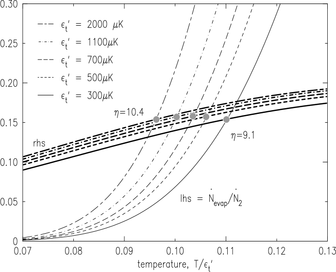
Figure A-8: Graphical solution of the heating/cooling balance equation, plotted for traps of various depths ${\epsilon_{t}}$. The bias energy is $\theta/{k_{B}}=34~{}\mu$K. The heavy lines are the right hand side (rhs) of equation A.28. The light lines are the left hand side. The solid dots indicate the equilibrium temperature for the various trap depths. At lower temperatures the equilibrium $\eta$ is smaller, indicating less efficient evaporation.

The equilibrium $\eta$ is larger at higher temperatures because the mean particle speed, and thus collision rate, is higher. The higher $\eta$ at higher temperatures indicates that evaporative cooling is more efficient there; fewer atoms are expended in the battle against heating caused by dipolar decay.

A.2.3 Forced Evaporative Cooling

The analysis above indicates that, for a given trap depth, a minimum temperature will be achieved which is set by the competition between heating and cooling. In order to cool the sample further the trap depth must be reduced. A comprehensive review by Ketterle and van Druten [56] of forced evaporation analyses the process in detail. For the experiments described in this thesis the trap depth is reduced by either lowering the magnetic confinement field at one end of the trap, or by reducing the frequency of an RF magnetic field that selectively removes the most energetic atoms. This second method is the focus of chapter 3.

A computer model (described in appendix D) has been used to evolve in time the total energy and total number of particles in the sample as it is cooled. Temperature and density are calculated along the way. The effects of changing the trap depth and changing the functional form of the trapping potential have been included. This model agrees well with experiments.

The rate at which the temperature of the gas can be changed is an important parameter. Luiten et al. [26] have shown that a classical gas with an energy distribution far from equilibrium will reasonably approximate a Maxwell-Boltzmann distribution after about three collision times. One therefore expects fluctuations of the energy distribution to dissipate on this time scale. To maintain quasi-equilibrium the trap depth and the trapping potential should thus be changed slowly compared to this collision time.

Since trapped atoms are a scarce commodity, a figure of merit for a cooling process is the amount of phase space compression achieved per atom lost. Far from quantum degeneracy the phase space density is the number of atoms per cubic thermal de Broglie wavelength, $D\equiv n\Lambda^{3}$. A useful measure of the cooling efficiency is the cooling exponent [56], which is the differential fractional change in phase space density per differential fractional change in population,

$$\gamma\equiv\frac{d\log D}{d\log N}.$$ (A.29)

A large, negative value indicates that the phase space density increases by a large factor for a decrease in population by only a small factor. Cooling exponents as large as $\gamma=-3$ have been observed [110].

In cooling clouds of alkali metal atoms, a process called “runaway evaporation” is observed, in which cooling of the sample leads to an increase in sample density because the atoms are more localized in the bottom of the trap. In turn, the increased density leads to an increased collision rate and faster evaporation. The cooling accelerates, a desirable phenomena because the number of atoms lost through background gas collisions during the time used to cool the sample is reduced when the cooling time is shorter. The conditions required for runaway evaporation are carefully explained by Ketterle et al. [56]. Runaway evaporation does not occur in clouds of trapped hydrogen because the dominant loss rate, due to dipolar relaxation, increases with increasing density with the same exponent as the evaporation rate. The ratio of the evaporation loss rate (“good” losses) to the dipolar decay loss rate (“bad” losses),

$$\frac{\dot{N}_{evap}}{\dot{N}_{2}}=\frac{\sigma\bar{v}V_{evap}}{gV_{2}}\sim 50e^{-\eta}(\eta-4.5)\sqrt{\frac{T}{1~{}\mu{\rm K}}},$$ (A.30)

is independent of density, depending only on $\sqrt{T}$ for a given $\eta$. The effective volumes for dipolar decay and evaporation used in equation A.30 are for $\phi\sim 1$ and $\eta>7$. From this equation we see that evaporation is more efficient at higher temperatures, as noted above.

Appendix B Fraction of Collisions Which Produce an Energetic Atom

In a collision between two atoms with a medium energy, what is the probability of creating an “energetic atom”, i.e. an atom with enough energy to escape the trap? Consider a collision between two distinguishable particles of identical mass $m$ and initial momenta ${\bf p}_{1}$ and ${\bf p}_{2}$. After the collision the momenta are labeled ${\bf q}_{1}$ and ${\bf q}_{2}$. The total and relative momenta are ${\bf P}=({\bf p}_{1}+{\bf p}_{2})$ and ${\bf p}={\bf p}_{1}-{\bf p}_{2}$, and similarly for ${\bf Q}$ and ${\bf q}$.

Conservation of momentum leads to the equation ${\bf P}={\bf Q}$. We orient the axes of the coordinate system so that ${\bf Q}=Q\hat{z}$ and we work in spherical coordinates. The total energy is

$$E_{0}=(P^{2}+p^{2})/4m.$$ (B.1)

Conservation of energy demands that $p^{2}=q^{2}$. We thus have four equations and six unknowns, leaving two undetermined coordinates, which will be labeled $\theta$ and $\phi$ in the description of

$${\bf q}=q\left\{\,(\hat{x}\cos\phi+\hat{y}\sin\phi)\,\sin\theta+\hat{z}\cos\theta\right\}.$$

After aligning the coordinate system we see that the there are two conserved scalar quantites, $P=Q$ and $p=q$. We can compute the fraction of this allowable phase space corresponding to various conditions by assuming that, in a collision, $\theta$ and $\phi$ may take any value with equal probability. We define the function $f(\theta,\phi)\;d\Omega$ as the volume of phase space within a differential solid angle $d\Omega$ of the given angles. Since the collisions are postulated to be independent of angle, we take $f(\theta,\phi)=f_{0}=1/4\pi$.

In the calculations to follow we scale the energies to the trap depth, $E_{t}$. We use the dimensionless variables $a\equiv q/\sqrt{4E_{t}m}$ and $b=Q/\sqrt{4E_{t}m}$. The total energy is then $E_{0}=E_{t}(a^{2}+b^{2})$.

We first find the fraction of phase space corresponding to one atom with energy greater than the trap depth. We call this an “energetic atom”. The condition is expressed as $E_{1}=q_{1}^{2}/2m>E_{t}$ or $E_{2}=q_{2}^{2}/2m>E_{t}$. Using ${\bf q}\cdot{\bf Q}=qQ\cos\theta$ and defining the “energy distribution” parameter $\xi\equiv ab\cos\theta$ we translate the conditon above to

$$|\xi|>1-E_{0}/2E_{t}.$$

The fraction of phase space (consistent with the given parameters $a$ and $b$) that corresponds to the existence of at least one energetic atom is then

$$G(Q,q) = \int_{|\xi|>1-E_{0}/2E_{t}}d\theta\sin\theta d\phi\;f(\theta,\phi)$$ (B.2)

$$= \int_{\alpha}^{1}du$$

where $u$ has been substituted for $\cos\theta$ and the lower limit on the integral is $\alpha=0$ if $E_{0}\geq 2E_{t}$ or, if $E_{0}<2E_{t}$, the smaller of $u_{0}\equiv(2-a^{2}-b^{2})/2ab$ and $1$. We obtain

$$G(a,b)=\left\{\begin{array}[]{ll}0&u_{0}\geq 1\\ 1-u_{0}&0<u_{0}<1\\ 1&u_{0}\leq 0\\ \end{array}\right.$$ (B.3)

This quantity may now be averaged over all the initial conditions of interest to obtain the average fraction of collisions which produce an energetic atom. The allowable initial conditions are that $E_{1}<E_{t}$, $E_{2}<E_{t}$, and $E_{0}>E_{t}$ since we assume both particles are initially trapped but there is enough total energy for one particle to escape. As we sum over all the possible initial states with the given $a$ and $b$, we must weight the average by the fraction of initial states which have both particles trapped. This factor is simply the volume of phase space left over from the above computation applied to the initial conditions, $1-G$. Since $P=Q$ and $p=q$, the average fraction is then

$$F=F_{0}\int_{E_{t}<E_{0}<2E_{t}}d^{3}{\bf Q}\>d^{3}{\bf q}\;G\,(1-G)$$

where $F_{0}$ is a normalization factor to be computed below. Exploiting the spherical symmetry and switching to scaled variables we obtain

$$F=F_{0}\>(4\pi)^{2}\>4E_{t}m\int_{0}^{\sqrt{2}}b^{2}db\int_{a_{min}}^{a_{max}}a^{2}da\;G(a,b)(1-G(a,b))$$ (B.4)

where $a_{min}=-b+\sqrt{2}$ and $q_{max}=\sqrt{2-b^{2}}$ are obtained from the condition that $0\leq u_{0}\leq 1$. The limits on the $b$ integral are chosen to keep the limits on the $a$ integral reasonable. The result is

$$F=F_{0}\>16\pi^{2}\>E_{t}m\>\frac{20-6\pi}{9}.$$

The normalization constant $F_{0}$ is simply the weighted integral over the allowable initial states,

$$F_{0}=\left(\int_{E_{t}<E_{0}<2E_{t}}d^{3}{\bf Q}\>d^{3}{\bf q}\;(1-G)\right)^{-1}.$$

We follow the same scheme, but note that when $u_{0}>1$ the integrand, $1-G$, remains at unity. We obtain

$$F_{0}=\left(16\pi^{2}E_{t}m\,\frac{4}{9}\right)^{-1}.$$

We conclude that the fraction of the collisions which will produce an energetic atom is

$$F=5-\frac{3\pi}{2}\approx 0.288.$$

The above calculation assumed that the probability of having any of the initial states was identical. In fact, the higher energy states are less likely than the lower energy states, as dictated by the Boltzmann factor. Into the above integrals, then, must be inserted the factor $\exp(-E_{0}/{k_{B}}T)=\exp(-\eta(a^{2}+b^{2}))$ where $\eta\equiv E_{t}/{k_{B}}T$. The $b$ integral must be computed numerically. We obtain behavior as indicated in Fig B-1.

Figure B-1: The fraction of collisions which produce an atom with enough energy to escape the trap. A truncated Maxwell-Boltzmann distribution of velocities is assumed. The parameter $\eta$ is the truncation energy divided by ${k_{B}}T$.

We see that for typical values of the parameter $\eta$, a collision which produces an energetic atom is an extremely rare event.

Another quantity of interest is the probability that an energetic atom which collides with another atom will becoming trapped. This is essentially the reverse of the process calculated above. We conclude that in the vast majority of collisions between a thermal atom and an energetic atom, neither atom will be energetic afterward.

Appendix C Behavior of Non-Condensed Fraction of a Degenerate Gas

In this appendix we consider a weakly interacting Bose gas of temperature $T$ and chemical potential $\mu\leq 0$ confined in a trap of depth ${\epsilon_{t}}$. A truncated Bose-Einstein energy distribution is assumed. Here we derive results that will be used in section 2.3. Truncation effects are important because of the shallow traps used for the experiments in chapter 5.

As discussed in section 2.2.2, the interactions in the condensate increase the chemical potential slightly above zero. The mean-field repulsion energy of the condensate deforms the effective trap shape slightly, moving the energy at the bottom of the trap from $\varepsilon=0$ to $\varepsilon=\mu$ and flattening the potential there. However, we ignore these effects on the thermal gas because for our experiments ${k_{B}}T\gg\mu$; the magnitude of the deformation is much smaller than the characteristic energy of the atoms.

C.1 Ideal Degenerate Bose Gas

C.1.1 Density

Here we calculate the density of the gas in a region of the trap with potential energy $\varepsilon$. We include truncation effects because, as will be shown in the experimental data in chapter 5, the typical $\eta$ is between 4 and 6 when the condensate is present. Integrating the occupation function over all the trapped momenta we obtain a density

$$n(\varepsilon;T,\mu,\epsilon_{t})=\frac{1}{h^{3}}\int_{0}^{p_{max}}\frac{4\pi p^{2}}{e^{(p^{2}/2m+\varepsilon-\mu)/{k_{B}}T}-1}\;dp$$ (C.1)

where $p_{max}^{2}/2m=\epsilon_{t}-\varepsilon$ is the largest allowable kinetic energy for atoms with potential energy $\varepsilon$. We separate the result of the integration into an expression for the density in an infinitely deep trap and a unitless correction factor $\Upsilon_{1/2}$ which accounts for truncation of the distribution. We obtain

$$n(\varepsilon;T,\mu,\epsilon_{t})=\frac{g_{3/2}(e^{(\mu-\varepsilon)/{k_{B}}T})}{\Lambda^{3}(T)}\;\Upsilon_{1/2}\left(\frac{\epsilon_{t}-\varepsilon}{{k_{B}}T},\frac{\mu-\varepsilon}{{k_{B}}T}\right).$$ (C.2)

The correction factor is

$$\Upsilon_{k}(\eta^{\prime},\mu^{\prime})\equiv\left\{\begin{array}[]{lll}\frac{\displaystyle\int_{0}^{\eta^{\prime}}\frac{x^{k}}{e^{x-\mu^{\prime}}-1}\;dx}{\displaystyle\int_{0}^{\infty}\frac{x^{k}}{e^{x-\mu^{\prime}}-1}\;dx}&;&\eta^{\prime}>0\\ 0&;&\eta^{\prime}\leq 0\\ \end{array}\right.$$ (C.3)

where $\eta^{\prime}$ is an effective unitless trap depth and $\mu^{\prime}$ is an effective chemical potential. In the limit of large $\eta^{\prime}$, $\Upsilon_{k}(\eta^{\prime},\mu^{\prime})=1$. The behavior of $\Upsilon_{1/2}$ is displayed in figure C-1.

Figure C-1: Behavior of the truncation correction factor $\Upsilon_{1/2}$, plotted for various effective chemical potentials. The largest deviations from unity occur for small $\eta^{\prime}$, corresponding to potential energies within a few ${k_{B}}T$ of the energy truncation point ${\epsilon_{t}}$. The range of $\mu^{\prime}$ shows how the correction factor changes between the classical ($\mu^{\prime}\ll-1$) and the degenerate quantum ($|\mu^{\prime}|\ll 1$) regimes. The asymptotic functional form for low and high $\mu^{\prime}$ can be seen.

As expected, the truncation correction factor is most pronounced at potential energies within a few ${k_{B}}T$ of the energy threshold $\epsilon_{t}$, for which $\eta^{\prime}$ is small. Also, for a nearly degenerate gas ($\mu^{\prime}$ small) the population is concentrated more at low energies so the effects of truncation are less important. For trap depths greater than $4{k_{B}}T$ the truncations effects can be neglected.

C.1.2 Kinetic Energy

The mean kinetic energy of the particles in a region of potential energy $\varepsilon$ is

$$\overline{K}(\varepsilon;T,\mu,\epsilon_{t})=\frac{1}{n(\varepsilon;T,\mu,\epsilon_{t})h^{3}}\int_{0}^{p_{max}}\frac{4\pi p^{2}}{e^{(p^{2}/2m+\varepsilon-\mu)/{k_{B}}T}-1}\;\frac{p^{2}}{2m}\;dp.$$ (C.4)

Again we break the result into an expression for $\overline{K}$ in an infinitely deep trap and a correction factor. We obtain

$$\overline{K}(\varepsilon;T,\mu,\epsilon_{t})=\left(\frac{3{k_{B}}T}{2}\right)\;\left(\frac{g_{5/2}(e^{\mu^{\prime}})}{g_{3/2}(e^{\mu^{\prime}})}\right)\;\left(\frac{\Upsilon_{3/2}(\eta^{\prime},\mu^{\prime})}{\Upsilon_{1/2}(\eta^{\prime},\mu^{\prime})}\right),$$ (C.5)

where $\eta^{\prime}=(\epsilon_{t}-\varepsilon)/{k_{B}}T$ and $\mu^{\prime}=(\mu-\varepsilon)/{k_{B}}T$. The first term is the classical term, obtained for a Maxwell-Boltzmann distribution. The middle term is the difference between classical and Bose statistics. The third term is the truncation correction, which is unity for deep traps. For $\mu^{\prime}=0$ the middle term is 0.513. This result is used in the calculation of the energy loss rate due to dipolar decay in section C.2. This result tells us that the velocity distribution of a degenerate Bose gas should be narrower than its classical counterpart, an effect observed in section 5.3.2.

C.1.3 Population

The number of atoms in the thermal gas is obtained by integrating the Bose occupation function, weighted by the density of states, over the trapped energy states:

$$N_{t}(T,\mu,\epsilon_{t})=\int_{0}^{\epsilon_{t}}\frac{\rho(\epsilon)}{e^{(\epsilon-\mu)/{k_{B}}T}-1}\;d\epsilon.$$ (C.6)

The lower bound on the integral is the bottom of the trap. For the analysis which follows the thermal gas will exist in the presence of a condensate, and so we set $\mu=0$. Specializing to the Ioffe-Pritchard trap, we obtain

$$N_{t}(T,\mu,\epsilon_{t})=A_{IP}({k_{B}}T)^{4}\frac{\pi^{4}+60\zeta(3)\phi}{15}\;A_{0}(\eta,\phi)$$ (C.7)

where $\zeta$ is the Riemann zeta function ($\zeta(3)=1.202$) and $A_{k}(\eta,\phi)$ is a correction factor for the truncation of the energy distribution:

$$A_{k}(\eta,\phi)=\frac{\displaystyle\int_{0}^{\eta}\frac{x^{2+k}(x+2\phi)}{e^{x}-1}\;dx}{\displaystyle\int_{0}^{\infty}\frac{x^{2+k}(x+2\phi)}{e^{x}-1}\;dx}.$$ (C.8)

The behavior of $A_{0}$ is shown in figure C-2.

Figure C-2: Behavior of the truncation correction factor $A_{0}$ as a function of scaled trap depth $\eta=\epsilon_{t}/{k_{B}}T$, plotted for various bias field energies $\phi=\theta/{k_{B}}T$. The asymptotic functional form for low and high $\phi$ can be seen.

C.1.4 Total Energy

The total energy of the thermal gas is derived in a manner analogous to the occupation:

$$E_{t}(T,\mu,\epsilon_{t})=\int_{0}^{\epsilon_{t}}\frac{\rho(\epsilon)}{e^{(\epsilon-\mu)/{k_{B}}T}-1}\;\epsilon\;d\epsilon.$$ (C.9)

We obtain, for a degenerate gas ($\mu=0$) in a Ioffe-Pritchard trap,

$$E_{t}(T,\epsilon_{t})=A_{IP}({k_{B}}T)^{5}\left(\frac{2\phi\pi^{4}}{15}+24\zeta(5)\right)\;A_{1}(\eta,\phi)$$ (C.10)

where $\zeta(5)=1.037$. The behavior of $A_{1}$ is shown in figure C-3.

Figure C-3: Behavior of the truncation correction factor $A_{1}$ as a function of scaled trap depth $\eta=\epsilon_{t}/{k_{B}}T$, plotted for various bias field energies $\phi=\theta/{k_{B}}T$. The asymptotic functional form for low and high $\phi$ can be seen.

The average energy per particle in the thermal gas, $\overline{E}_{t}$, is then

$$\overline{E}_{t}(T,\epsilon_{t})=\frac{E_{t}}{N_{t}}={k_{B}}T\;B(\phi)\frac{A_{1}(\eta,\phi)}{A_{0}(\eta,\phi)}$$ (C.11)

where

$$B(\phi) \equiv 2\frac{\phi\pi^{4}+180\zeta(5)}{\pi^{4}+60\zeta(3)\phi}$$ (C.12)

$$\simeq 2.701\frac{\phi+1.916}{\phi+1.351}$$

is a factor that indicates whether the trap is predominantly linear or harmonic in the radial direction. This average energy is shown in figure C-4.

Figure C-4: The average energy per particle in the thermal portion of a degenerate Bose gas as a function of scaled trap depth $\eta=\epsilon_{t}/{k_{B}}T$, plotted for various bias field energies $\phi=\theta/{k_{B}}T$. For low $\phi$ the potential is linear in the radial direction. More energy can be carried as radial potential energy for low $\phi$ than for large $\phi$, which corresponds to harmonic potentials.

For a classical gas the average energy per quadratic degree of freedom is ${k_{B}}T/2$, but for a degenerate Bose gas the energy is less. For large $\phi$ the potential is harmonic and there are six quadratic degrees of freedom, implying a mean energy of $3{k_{B}}T$ for a classical gas; for a degenerate Bose gas the mean energy is 2.7 ${k_{B}}T$. The difference between the classical and degenerate Bose results (3-2.7) is not as great as the factor $\sim 0.5$ mentioned for $\mu^{\prime}=0$ in the discussion of equation C.5. This is because in calculating the mean kinetic energy an average is made over all the atoms in the trap with their many effective chemical potentials. Atoms far from the center of the gas have $\mu^{\prime}\ll-1$, and are essentially in the classical regime.

C.2 Dipolar Decay

The rate at which atoms leave the thermal gas through dipolar decay is calculated by integrating $\dot{n}=-gn^{2}$, over the volume of the gas. For a degenerate gas in the IP trap we obtain a two-body loss rate

$$\dot{N}_{2,t}(T,\epsilon_{t}) = \int_{0}^{\epsilon_{t}}\varrho(\varepsilon)(-g)n^{2}(\varepsilon;T,\mu=0,\epsilon_{t})\;d\varepsilon$$ (C.13)

$$= -\frac{({k_{B}}T)^{5/2}{\cal A}_{IP}g}{\Lambda^{6}}\;Q_{1}(\phi,\eta)$$

where $Q_{1}$ is the (unitless) integral of the density squared, and includes truncation effects:

$$Q_{1}(\phi,\eta)=\int_{0}^{\eta}\sqrt{x}(x+\phi)\;g_{3/2}^{2}(e^{-x})\Upsilon_{1/2}^{2}(\eta-x,-x)\;dx.$$ (C.14)

The behavior of $Q_{1}$ is shown in figure C-5.

Figure C-5: Behavior of the squared density integral $Q_{1}$ as a function of scaled trap depth $\eta=\epsilon_{t}/{k_{B}}T$, plotted for various bias field energies $\phi=\theta/{k_{B}}T$. In the figure $Q_{1}$ is scaled by $0.337+0.589\phi$, the high $\eta$ asymptote.

The rate at which energy leaves the thermal gas through dipolar decay is

$$\dot{E}_{2,t}(T,\epsilon_{t}) = \int_{0}^{\epsilon_{t}}\varrho(\varepsilon)(-g)n^{2}(\varepsilon;T,\mu=0,\epsilon_{t})\;\left(\varepsilon+\gamma(\varepsilon)\right)\;d\varepsilon$$ (C.15)

$$= -\frac{({k_{B}}T)^{7/2}{\cal A}_{IP}g}{\Lambda^{6}}\;Q_{2}(\phi,\eta)$$

where

$$Q_{2}(\phi,\eta) = \int_{0}^{\eta}\sqrt{x}(x+\phi)\;g_{3/2}^{2}(e^{-x})\Upsilon_{1/2}^{2}(\eta-x,-x)\;$$ (C.16)

$$\times\left(x+\frac{3}{2}\frac{g_{5/2}(e^{-x})}{g_{3/2}(e^{-x})}\frac{\Upsilon_{3/2}(\eta-x,-x)}{\Upsilon_{1/2}(\eta-x,-x)}\right)dx$$

The behavior of $Q_{2}$ is shown in figure C-6.

Figure C-6: Behavior of the dipolar decay energy loss integral $Q_{2}$ as a function of scaled trap depth $\eta=\epsilon_{t}/{k_{B}}T$, plotted for various bias field energies $\phi=\theta/{k_{B}}T$. In the figure $Q_{2}$ is scaled by $0.819+1.064\phi$, the high $\eta$ asymptote. The asymptotic functional form can be seen for high $\phi$.

The average energy carried away by each particle that is lost through dipolar relaxation is then $C_{2}{k_{B}}T={k_{B}}TQ_{2}/Q_{1}$, and is shown in figure C-7.

Figure C-7: Average energy of atoms lost from thermal portion of a degenerate gas through dipolar decay, in units of ${k_{B}}T$, plotted for $\mu=0$ and various bias energies $\phi=\theta/{k_{B}}T$. The asymptotic functional forms for small and large $\phi$ are apparent.

As expected, the average energy lost per particle through dipolar relaxation is less than $\overline{E}$, the average energy per particle throughout the sample (compare figure C-7 with figure C-4), and thus dipolar relaxation leads to heating. Compared to the Maxwell-Boltzmann distribution, the Bose-Einstein distribution has more particles at lower energy. We thus expect $C_{2}$ to be smaller, as is seen by comparing figure C-7 to figure A-5.

Appendix D Model of the Dynamics of the Non-Degenerate Gas

This appendix describes a computer model of the dynamics of the trapped gas, including evaporation, dipolar decay, and changes of the trap shape and depth. The C source code is available.

D.1 Overview

We desire a general purpose computer model of the time evolution of our trapped gas to assist in choosing paths through parameter space toward BEC. Previous models [17] employed approximations that are not valid at the low temperatures we wish to access and are not easily adaptable to the more complicated trap shapes we wish to employ.

D.1.1 Approximations

The primary approximation is that the phase space distribution function for the gas is always a Maxwell-Boltzmann truncated at the trap depth. Luiten et al. [26] have confirmed this approximation for slow evaporation. This approximation is valid as long as two additional assumptions are valid: (a) instantaneous ergodicity and (b) instantaneous removal of energetic atoms. The validity of these approximations depends on some time scales. For approximation (a) we need the time required for the gas to re-equilibrate to be short compared to the speed at which the trap shape and depth are changed. For approximation (b) we need the energetic atoms to be removed quickly compared to the energy redistribution time. These are the approximations described in section A.1.1.

D.1.2 Describing the Trap

We make no approximations about the trap shape. Instead the trap is described by energy and potential energy density-of-states functions ($\rho(\epsilon)$ and $\varrho(\varepsilon)$) which may involve any number of parameters, all (possibly) time dependent. The energy truncation point is also given as a time-dependent parameter.

D.2 Statistical Mechanical Description of the Gas

D.2.1 Variables

We describe the trap by an evaporation energy threshold, ${\epsilon_{t}}(t)$, and the density of states functions and their set of (time dependent) parameters, $\alpha_{\sigma}(t)$. These are our independent variables. Some function is given by the user to relate these trap shape parameters to time, the ultimate independent variable.

The primary dependent variables are $E$ and $N$, the total energy and total population of the sample. At each time step during the evolution of the trapped gas we calculate changes to the total energy, $dE$, and to the total number of atoms in the trap, $dN$. The new value for $T$ may then be calculated from $E$. If the form of $\rho(\epsilon)$ is known, it is often possible to analytically relate $T$ to $E$. Otherwise $T$ must be determined numerically, as is done in this model. The density parameter $n_{o}$ is trivially related to $N$ by equation A.13.

D.2.2 Computing Properties of the Gas

The population, $N$, total energy, $E$, and density $n({\bf r})$ are computed as described in section A.1.

For notational simplicity, we introduce the functions

$$\psi_{n}\equiv\int_{0}^{{\epsilon_{t}}}d\epsilon\,\rho(\epsilon)\,\epsilon^{n}\,e^{-\epsilon/{k_{B}}T}$$ (D.1)

and

$$\varphi_{n}\equiv\int_{0}^{{\epsilon_{t}}}d\epsilon\,\rho(\epsilon)\,\epsilon^{n}.$$ (D.2)

The Helmholtz free energy is given by $A=-{k_{B}}T\log{{\cal Z}}_{N}$, where ${{\cal Z}}_{N}$ is the $N$-particle partition function defined below equation A.8. We can define a “single particle” free energy

$$A_{1}\equiv-{k_{B}}T\log{{\cal Z}}$$

so that $A=NA_{1}+{k_{B}}T\log N!.$ The entropy is

$$S=-\left.\frac{\partial A}{\partial T}\right|_{V}$$ (D.3)

To keep ${V_{eff}}$ constant, we replace ${{\cal Z}}$ with ${V_{eff}}/\Lambda^{3}$ (using equation A.13) to obtain

$$S={k_{B}}\left(N\log{{\cal Z}}+\frac{3N}{2}-\log N!\right).$$ (D.4)

D.3 Treatment of Physical Effects

The model accounts for cooling due to evaporation, heating due to two-body spin relaxation, adiabatic trap shape changes, and the skimming of energetic atoms as the energy threshold is lowered. The finite trap depth is fully integrated into the model.

At each time step we calculate

$$\dot{E}=\dot{E}_{evap}+\dot{E}_{2}+\dot{E}_{trap}+\dot{E}_{skim}$$ (D.5)

and

$$\dot{N}=\dot{N}_{evap}+\dot{N}_{2}+\dot{N}_{skim}.$$ (D.6)

Each of these terms is explained below.

D.3.1 Evaporation

Luiten et al. [26] have described the evaporation process, starting from the kinetic equation. We summarize their results here. Following section A.2.1, the particle loss rate due to evaporation is

$$\dot{N}_{evap}=-n_{o}^{2}\,\sigma\,\bar{v}\,V_{evap}$$ (D.7)

where $\sigma$ is the collision cross section, $\bar{v}=\sqrt{8{k_{B}}T/\pi m}$ is the mean speed,

$$V_{evap} = \Lambda^{3}e^{-\eta}\int_{0}^{{\epsilon_{t}}}d\epsilon\,\rho(\epsilon)\left[(\eta-1-\epsilon/{k_{B}}T)e^{-\epsilon/{k_{B}}T}+e^{-\eta}\right]$$ (D.8)

$$= \Lambda^{3}e^{-\eta}\left((\eta-1)\psi_{0}-\frac{\psi_{1}}{{k_{B}}T}+\varphi_{0}e^{-\eta}\right)$$

is the effective volume for evaporation, and $\eta\equiv{\epsilon_{t}}/{k_{B}}T$. The energy loss rate due to evaporation is

$$\dot{E}_{evap}=-n_{o}^{2}\sigma\bar{v}\left\{({\epsilon_{t}}+{k_{B}}T)V_{evap}-{k_{B}}TX_{evap}\right\}$$ (D.9)

where

$$X_{evap} = \Lambda^{3}e^{-\eta}\int_{0}^{{\epsilon_{t}}}d\epsilon\,\rho(\epsilon)\,\left[e^{-\epsilon/{k_{B}}T}-(\eta+1-\epsilon/{k_{B}}T)e^{-\eta}\right]$$ (D.10)

$$= \Lambda^{3}e^{-\eta}\left(\psi_{0}-(\eta+1)\varphi_{0}e^{-\eta}+\frac{\varphi_{1}}{{k_{B}}T}e^{-\eta}\right)$$

D.3.2 Dipolar Spin Relaxation

The particle and energy loss rates $\dot{N}_{2}$ and $\dot{E}_{2}$ due to dipolar relaxation are given by equations A.20 and A.22 in section A.1.4.

D.3.3 Trap Shape Changes

We assume that the trap shape is changing slowly compared to the transit time of an atom across the trap. Trap shape changes are then adiabatic. We can use $dS=0$ to compute $dT$ from changes in the parameters to $\rho(\epsilon)$, and eventually obtain $dE$.

We break $dE$ into its constituents

$$dE=\left.\frac{\partial E}{\partial T}\right|_{\alpha}dT\,+\sum_{\sigma}\left.\frac{\partial E}{\partial\alpha_{\sigma}}\right|_{T}d\alpha_{\sigma}$$ (D.11)

where the first partial derivative is done at constant trap shape and the sum in the second term is over all the trap shape parameters. Since the process is adiabatic, $dS=0$. From equation D.4 we see that if $dS=0$ and $N$ is fixed we must have $d{{\cal Z}}=0$. Then we may find $dT$ by writing out $d{{\cal Z}}$. We obtain

$$dT=-\frac{\sum_{\sigma}\left.\frac{\partial{{\cal Z}}}{\partial\alpha_{\sigma}}\right|_{T}d\alpha_{\sigma}}{\left.\frac{\partial{{\cal Z}}}{\partial T}\right|_{\alpha_{\sigma}}}$$ (D.12)

Note that

$$\left.\frac{\partial\psi_{n}}{\partial T}\right|_{\alpha}=\frac{\psi_{n+1}}{{k_{B}}T^{2}}.$$ (D.13)

Remembering that $E=N\psi_{1}/\psi_{0}$ we get

$$\dot{E}_{trap}=\frac{E}{\psi_{1}}\sum_{\sigma}\left(\frac{\partial\psi_{1}}{\partial\alpha_{\sigma}}-\frac{\psi_{2}}{\psi_{1}}\frac{\partial\psi_{0}}{\partial\alpha_{\sigma}}\right)\dot{\alpha}_{\sigma}.$$ (D.14)

In practice the partial derivatives are evaluated numerically.

D.3.4 Skimming Energetic Atoms

As the trap evaporation threshold is lowered, atoms are skimmed from the top of the energy distribution. Using equation A.7 we calculate

$$dN_{skim} = \left.\frac{\partial N}{\partial{\epsilon_{t}}}\right|_{T,\alpha_{\sigma}}d{\epsilon_{t}}$$

$$\dot{N}_{skim} = \frac{N\rho({\epsilon_{t}})e^{-\eta}}{\psi_{0}}\dot{\epsilon}_{t}$$ (D.15)

and

$$\dot{E}_{skim}={\epsilon_{t}}\,\dot{N}_{skim}.$$ (D.16)

D.4 Software Implementation

The evaporation simulator is a set of routines which numerically integrate the differential equations for $E$ and $N$ through time. A user of these routines must write C routines that describe the trap to the integration routines. The description takes the form of an energy density of states, a potential energy density of states, and an energy threshold above which the energy distribution is truncated. Other code (described below) is also expected to parse the command line and do initialization. Ideally, all of the information that specializes the general evaporation routines to a specific trap and ramp function is contained in a single file in the directory specialized. This file is mentioned in the top level Makefile. Henceforth this file will be referred to as userfile.

Information about the trap is passed to the evaporation simulation routines in a data structure,

mytrap1, defined in {\tt prog.h}.  The
components of this data structure are pointers to functions and
arrays.  The data structure is a global variable, and is initialized
by the routine \verb

initialize_mytrap1 in userfile. This routine is called at the very beginning of the program.

D.4.1 Program Flow

Execution of the program flows as follows. First, initialize_mytrap() is called to set up the data structure. Then a routine, pointed to by

mytrap1, is invoked to parse the command
line and stash user-provided information into the appropriate arrays.  The
differential equation integrator is then started.  It steps $E$ and
$N$ through time using the Runge-Kutta routines from Numerical Recipes
\cite{numerical.recipes}.  At each time step the routines from {\em
userfile} are used as follows.  First, the threshold and parameters
used for calculating the density of states are calculated.  These
might correspond to magnet currents or rf field frequencies, as
computed for controlling the experiment.  These values are printed to
a log file.  Since these parameters may often be manipulated into a
form that economizes computation when calculating the density of
states, another routine, pointed to by \mytrap, is invoked to do this.
Finally, we are ready to calculate $\psi_n$ and $\varphi_n$ for this
instant.  The new temperature and density are calculated.  The effects
of evaporation, relaxation, skimming, and adiabatic trap shape changes
are determined, and we are ready for the next step.
\subsection{Data Structure}
The data structure \mytrap \ is referenced often is these calculations,
and is the link between user-supplied routines and the general
simulation machinery.  The entries in the data structure are:
\begin{list}{}{}
\item{{\tt parse}} Pointer to a function which parses the command
line, obtaining the initial density and temperature of the simulated
gas, and the duration of the simulation.  This information is returned
to the simulator.  Further information might be the beginning and
ending currents in certain magnets, shape factors for ramps, etc.,
which would be used to specify the trap shape at each instant of time.
\item{{\tt threshold}} Pointer to a function that gives the energy
threshold (atoms with more than this energy are assumed to escape from
the trap), as a function of time.
\item{\verb

calc_dos_params1 Pointer to a function which calculates, at a given time, the parameters used to calculate the density of states. The values calculated here will be printed in the log file for each time step. n_dos_params An integer, giving the number of density of states parameters calculated by calc_dos_params. These are printed in the log file. precalculate Pointer to a function which manipulates the density of states parameters to speed up actual calculation of the density of states. For example, in a Ioffe trap the density of states is proportional to the square root of the radial confinement field. This square root may be calculated here in this routine. edos A pointer to a routine which returns the energy density of states at a given energy. pedos A pointer to a routine which returns the potential energy density of states at a given energy. trapspecs An array of information used (possibly) by calc_dos_params and threshold. These data are not touched by the simulator. The only C file that looks at these is userfile. ntrapspecs Size of the array trapspecs. Only used in file userfile. Several examples of userfile exist, and may be copied and hacked.

Appendix E Bose-Einstein Velocity Distribution Function

To find the one-dimensional velocity distribution function which is used in calculating the Doppler-sensitive lineshape observed in section 5.3.2 one should use the Bose-Einstein (BE) occupation function instead of the more convenient Maxwell-Boltzmann (MB) occupation function. For a gas at temperature $T$ and chemical potential $\mu$ the occupation function is

$$f(\epsilon;T,\mu)=\frac{1}{e^{(\epsilon-\mu)/\kb T}-1}$$ (E.1)

In this appendix we derive the BE one-dimensional velocity distribution function and use it to calculate characteristic spectral lineshapes. Truncation effects for a trap of depth $\ethr$ are included, but shown to be small when the laser beam intersects the middle of the trap and preferentially excites atoms from the deepest part of the trap. In this case, quantum degeneracy is shown to narrow the spectrum.

E.1 Velocity Distribution

The one-dimensional momentum distribution function is obtained in a way analogous to the density, in equation C.2, but the momentum integral is over only two dimensions. We define $f_{p}(p_{z})\>dp_{z}$ as the probability of an atom having a momentum along the $\hat{z}$ axis within a range $dp_{z}$ of $p_{z}$; the normalization is 1. The distribution is

$$f_{p}(p_{z})=\frac{\displaystyle\int_{0}^{p_{\perp,max}}\frac{2\pi p_{\perp}}{e^{(p_{\perp}^{2}/2m+p_{z}^{2}/2m+\varepsilon-\mu)/\kb T}-1}\;dp_{\perp}}{\displaystyle\int_{0}^{p_{max}}\frac{4\pi p^{2}}{e^{(p^{2}/2m+\varepsilon-\mu)/\kb T}-1}\;dp}$$ (E.2)

where $p_{\perp}$ is the momentum perpendicular to $\hat{z}$ and $p_{\perp,max}^{2}/2m=\epsilon_{t}-\varepsilon-p_{z}^{2}/2m$ is the maximum allowable kinetic energy perpendicular to $\hat{z}$. The denominator is $h^{3}n(\varepsilon;T,\mu,\epsilon_{t})$, calculated above. The numerator can be broken into an expression which neglects truncation and a correction factor $\Upsilon_{0}$ defined in equation C.3. We obtain

$$f_{p}(p_{z};T,\mu,\epsilon_{t},\varepsilon) = \frac{-2\pi m\kb T}{h^{3}n(\varepsilon;T,\mu,\epsilon_{t})}\log\left(1-\exp\left(\frac{\mu-\varepsilon-p_{z}^{2}/2m}{\kb T}\right)\right)$$ (E.3)

$$\times\Upsilon_{0}\left(\frac{\epsilon_{t}-\varepsilon-p_{z}^{2}/2m}{\kb T},\frac{\mu-\varepsilon-p_{z}^{2}/2m}{\kb T}\right)$$

The behavior of $\Upsilon_{0}$ is shown in figure E-1.

Figure E-1: Behavior of the truncation correction factor $\Upsilon_{0}$ as a function of effective trap depth $\eta^{\prime}$, plotted for various effective chemical potentials $\mu^{\prime}$.

For large $\eta^{\prime}$ truncation is unimportant and $\Upsilon_{0}=1$. The velocity distribution function is $f_{v}(v_{z})=mf_{p}(mv_{z})$. Figure E-2 shows this distribution function for various potential energies in the trap.

Figure E-2: One dimensional velocity distribution function, plotted for regions with various potential energies $\varepsilon$ (listed in units of $\kb T$). The sample temperature is $T=50~{}\mu$K, the chemical potential is $\mu=-2\times 10^{-7}\kb T$, and the trap depth is $6\kb T$. The inset reveals part of the $\varepsilon=0$ distribution that is not visible in the main figure.

At higher potentials the effective chemical potential becomes more negative, and the distributions look more classical. Only very near the trap minimum is there significant clumping of the velocities around zero. Figure E-3 directly compares the quantum velocity distribution (small $\mu$) with the classical distribution (large $\mu$).

Figure E-3: Comparison of one dimensional velocity distributions for samples near to (far from) quantum degeneracy, having chemical potential $\mu/\kb T=-2\times 10^{-7}$ ($\mu/\kb T=-20$), plotted with heavy (light) lines. The sample temperature is $T=50~{}\mu$K. The trap depth is $6\kb T$. The velocity distribution for each chemical potential is plotted for three different potential energies, listed in units of $\kb T$. For the $\varepsilon=5$ case the two lines overlap; also, truncation effects are clear because of the shallow effective depth.

As expected, the classical velocity distribution at $\varepsilon=0.1\kb T$ and $\varepsilon=1\kb T$ are nearly identical, but differ substantially from their quantum counterparts. For $\varepsilon=5\kb T$ the classical and quantum distributions are nearly identical because even the degenerate gas becomes dilute at this high potential energy. Truncation effects are important, as evidenced by the sharp cutoff of the velocity distribution.

E.2 Spectral Signature of Velocity Distribution

The Doppler-sensitive spectrum is a direct measure of the one-dimensional velocity distribution function $f_{v}(v_{z})$ through the (radian) frequency shift $\Delta={\bf k}\cdot{\bf v}$, where ${\bf k}=2\pi\hat{z}/\lambda$ is the wavevector of the radiation and $\lambda=243.2$ nm. The spectrum, $S(\Delta)$, is given by considering the spectrum of the atoms at each potential energy in the trap:

$$S(\Delta)=S_{0}\int_{0}^{\epsilon_{t}}d\varepsilon\;\varrho(\varepsilon)n(\varepsilon)\;\int_{-v_{max}}^{v_{max}}dv_{z}f_{v}(v_{z})\delta(\Delta-kv_{z})$$ (E.4)

where $mv_{max}^{2}/2\equiv\epsilon_{t}-\varepsilon$ is the maximum kinetic energy allowable for atoms with potential energy $\varepsilon$. The inner integral vanishes if $|\Delta/k|>v_{max}$. The upper integration limit on the outer integral thus becomes $\varepsilon_{max}=\epsilon_{t}-m\Delta^{2}/2k^{2}$. The spectrum is

$$\displaystyle S(\Delta)= \displaystyle\frac{S_{0}}{h\Lambda^{2}}\int_{0}^{\varepsilon_{max}}d\varepsilon\varrho(\varepsilon)\log\left(1-e^{(\mu-\varepsilon-m\Delta^{2}/2k^{2})/\kb T}\right)$$ (E.5)

$$\displaystyle\times\Upsilon_{0}\left(\frac{\epsilon_{t}-\varepsilon-m\Delta^{2}/2k^{2}}{\kb T},\frac{\mu-\varepsilon-m\Delta^{2}/2k^{2}}{\kb T}\right)$$

This calculation has assumed uniform laser illumination of the sample, has ignored coherence effects for atoms that pass repeatedly through the laser beam during excitation, has assumed all atoms are driven for identical durations, and has neglected the cold-collision frequency shift. The non-uniform laser illumination can be inserted into equation E.5 as a factor $R(\varepsilon)$, an average of the square of the laser intensity over the surface of constant potential energy $\varepsilon$ in a trap potential $V({\bf r})$,

$$R(\varepsilon)I_{0}^{2}=\frac{1}{\varrho(\varepsilon)}\int d^{3}{\bf r}\;I^{2}(\rho,z)\;\delta(\varepsilon-V({\bf r}))$$ (E.6)

where $I(\rho,z)=I_{0}\exp(-2\rho^{2}/\omega^{2}(z))$ describes the spatial dependence of the intensity of a Gaussian beam [103]; the beam radius a distance $z$ from the focus is $\omega(z)=\omega_{0}\sqrt{1+(z/d)^{2}}$ where $\omega_{0}$ is the waist radius and $d=\pi\omega_{0}^{2}/\lambda$ is the divergence length. We assume the beam focus is at the center of the trap and the beam is oriented parallel to the cylindrical symmetry axis of the trap. For a Ioffe-Pritchard trap potential $V(\rho,z)=\sqrt{(\alpha\rho)^{2}+(\beta z^{2}+\theta)^{2}}-\theta$, we obtain

$$R(\varepsilon)=\sqrt{\frac{\beta}{\varepsilon}}\;\int_{0}^{\sqrt{\varepsilon/\beta}}dz\exp\left\{-\frac{4}{\alpha^{2}\omega_{0}^{2}}\frac{(\varepsilon+\theta)^{2}-(\beta z^{2}+\theta)^{2}}{1+(z/d)^{2}}\right\}$$ (E.7)

This average has been calculated for the trap shape of immediate interest for the experiments described in this thesis. See figure E-4.

Figure E-4: The average of the square of the laser beam intensity on an equipotential surface of energy $\varepsilon$, plotted for various beam waist radii $\omega_{0}$. The trap has radial energy gradient $\alpha/\kb=16$ mK/cm, axial curvature $\beta/\kb=25~{}\mu{\rm K/cm^{2}}$, and bias $\theta/\kb=34~{}\mu$K. At large $\varepsilon$ the average vanishes very slowly because the beam diverges and illuminates more of the surface.

The laser beam primarily excites the atoms at the bottom of the trap where the beam intensity is largest. The energy distribution truncation effects are thus not very important, and the shape of the velocity distribution is well approximated by $-\log(1-\exp((\mu-\varepsilon-mv_{z}^{2}/2)/\kb T))$. Because the the effective chemical potential is small for these atoms, however, quantum effects can be important. Figure E-5

Figure E-5: Expected Doppler-sensitive lineshape for a gas near to (far from) the quantum degenerate regime, plotted for samples at various temperatures. The thick (thin) lines are for samples with chemical potential $\mu/\kb=-1\times 10^{-4}(-5\times 10^{2})~{}\mu$K, corresponding to the degenerate (non-degenerate) regime. For these calculations $\ethr=300~{}\mu$K, $\alpha=16$ mK/cm, $\beta=25~{}\mu{\rm K/cm^{2}}$, $\theta=34~{}\mu$K, and $\omega_{0}=48~{}\mu$m.

shows calculations of the lineshape, using equation E.5 and including $R(\varepsilon)$, for samples in the quantum degenerate regime at various temperatures for a set of trap parameters of immediate interest to this experiment. We see that the distributions are significantly narrower than those arising from samples far from quantum degeneracy. If the spectrum for a degenerate sample is fit to the distribution expected for a non-degenerate sample, the quoted temperature will be about 40% too low; the actual temperature is about 1.6 times higher for the conditions of immediate interest in our experiment.

Appendix F Model of the Dynamics of the Degenerate Gas

F.1 Overview

This appendix describes a computer model of the dynamics of the degenerate trapped gas, including evaporation and dipolar decay losses from the condensate and thermal gas. As depicted in figure 2-2, the trapped gas is modeled as a system composed of two tightly coupled components, the thermal gas and the condensate. We assume the loss rates from the system are slow compared to the rates of transferring particles and energy between the two components. A dynamical equilibrium is thus postulated. The results of this model are shown in figure 5-11. The trap shape is assumed to be static and of the Ioffe-Pritchard form. The depth is fixed. The Bose-Einstein occupation function is used for calculation of dipolar decay losses from the thermal gas, and the Thomas-Fermi condensate wavefunction is the basis for calculations of loss from the condensate. The particle and energy loss rates due to evaporation should be calculated using a quantum kinetic theory derived from the quantum Boltzmann transport equation. This approach would correctly include the Bose statistics. As a very simple approximation to the desired, but complicated, formulation, we simply apply the evaporation rates calculated for a Maxwell-Boltzmann distribution by Luiten et al. [26] (equations in section A.2.1). One expects a lower evaporation rate near quantum degeneracy because atom energies are distributed to lower energies relative to the thermal energy $\kb T$ than is typical in a classical gas. Roughly speaking, the effective $\eta$ is larger. Another way to think about the situation is to realize that collisions which lead to evaporation occur preferentially among higher energy atoms. As shown in figure 2-1, the Maxwell-Boltzmann distribution calls for many more atoms in these regions of higher energy than does the Bose-Einstein distribution in the degenerate regime. We therefore reduce the evaporation rate by the adjustable factor ${\cal F}$ of order $0.4$. This ${\cal F}$ is the factor mentioned in figure 5-11. Note that the rate of evaporation is reduced, but the energy of the escaping atoms is still approximately $(\eta+1)\kb T$.

F.2 Simulation Details

The input to the simulation is the initial temperature of the thermal gas and the initial condensate population (the proper thermodynamic parameters are $T$ and $\mu$; the chemical potential is directly linked to the peak condensate density, which is directly connected to the condensate population). The trap shape and depth ($\alpha,\beta,\theta,\ethr$) are additional parameters. Finally, a one body loss rate with time constant $\tau_{1}$ is specified. Using this input, the program calculates the total occupation of the trap, $N_{T}$, and the total energy, $E_{T}$, using equations C.6, C.9, and 2.14, and the condensate energy $E_{c}=\mu N_{c}=n_{p}U_{0}N_{c}$. It is the total energy and the total population that is evolved in time. At each time step the temperature is found by numerically solving equation C.9 for the total energy of the thermal gas. We assume $\mu=0$ for the thermal gas during the entire simulation. If we allowed $\mu$ to vary, then two equations would have to be consistently solved numerically, one for $N_{t}$ and one for $E_{t}$ (possible, but more difficult). Once the temperature is found, the occupation of the thermal gas is calculated. The condensate occupation is the total trap occupation minus the thermal occupation, $N_{c}=N_{T}-N_{t}$ (we postulate equilibrium between the thermal gas and the condensate, a questionable assumption as discussed in section 2.3.3). The particle and energy loss rates due to dipolar relaxation from the thermal gas and condensate are calculated using equations C.13 and C.15. Possible one-body losses are added. The particle and energy loss rates due to evaporation from the thermal gas are calculated for a classical gas of the same peak density as the Bose gas being simulated, $n_{o}=2.612/\Lambda^{3}(T)$. These rates are multiplied by the correction factor ${\cal F}$. The sum of all the particle and energy loss rates for the given time step is returned to the differential equation stepper routine. The simulation is stepped through time using the Romberg integration technique [111]. Errors in $N_{T}$ and $E_{T}$ are maintained below the $10^{-5}$ level.

F.3 Improvements

One important improvement would be to determine the evaporation rate using the quantum Boltzmann equation, which is based on the correct quantum occupation function. This has been done very recently [112]. Further improvements would include treatment of the finite feeding rate of the condensate from the thermal gas. This bottleneck should be playing a role for the largest condensates in this thesis, as suggested in section 2.3.3.

Appendix G Trap Shape Uncertainties

In order to calculate various properties of the thermal gas and condensate, it is necessary to combine measurements (of density and temperature, for example) with knowledge of the trap shape. In principle the trap shape can be calculated simply from the Biot-Savart law. In practice various complications arise. In this appendix we discuss these complications and estimate their effect on the trap shape. We conclude that the trap parameters (radial gradient $\alpha$ and axial curvature $\beta$) should have uncertainties of less than 20%. The trap shapes used for the experiments in this thesis are created by currents in 17 superconducting coils. Various compensation schemes are employed to produce steep gradients and large curvatures along the $z$ axis, and shim coils are used to adjust the bias field. One source of uncertainty is knowledge of the precise geometry of the coils. Additional uncertainties exist because fields of unknown strength and direction arise from trapped fluxes [17] and magnetized materials in the cryostat. We first address the stray fields: how can these stray fields influence the trap shape? Let us consider the influence of stray fields on the three Ioffe-Pritchard trap parameters, $\alpha$, $\beta$, and $\theta$. We label the three space coordinates $x,y,z$, and assume the trap exhibits cylindrical symmetry about the $z$ axis. A uniform field perpendicular to the $z$ axis will shift the location of the trap minimum in the plane, but will not affect $\alpha$, $\beta$, or $\theta$. A uniform field parallel to the $z$ axis will shift $\theta$, but not affect $\alpha$ or $\beta$. A gradient field with strength $B=s\>x$ ($s$ is the gradient strength) aligned perpendicular to the $z$ axis will add linearly with $\alpha$, but will not affect $\beta$ or $\theta$. A field with strength $B=s\>z$ aligned parallel to the $z$ axis will move the trap minimum along the axis and shift $\theta$, but will not affect $\beta$. A field with strength $B=s\>z$ aligned perpendicular to the $z$ axis will tip the trap symmetry axis away from the $z$ axis, but not affect any parameters directly. Finally, a field parallel to the $z$ axis and with strength $B=s\>x$ will bow the trap and directly perturb all three parameters. Defining the unitless parameter $\epsilon=\sqrt{1+(\mu_{B}s/\alpha)^{2}}$, we find that $\alpha\rightarrow\epsilon\alpha$, $\beta\rightarrow\beta/\epsilon$, and $\theta\rightarrow\theta/\epsilon$. In the traps of immediate interest in this thesis, the samples are short (a few cm) and very narrow (less than 1 mm in diameter). The radial gradient fields are large ($\sim 10^{2}$ G/cm), and sources of stray fields are far (several cm) from the sample. Thus, we expect only very weak perturbations to the gradient parameter $\alpha$ and the curvature $\beta$. The parameter $\theta$ is easily perturbed, but we can measure it directly, as described in section 4.2.4. Trapped fluxes are expected to exist on the 1 G level, but the distance from the sources (superconducting wires) to the trap should cause these fields to appear as simple gradients, which have been shown above to only slightly perturb $\beta$ and $\alpha$. Magnetic materials in the cryostat could produce large fields ($\sim 10-100$ G), but they are very far away and the field should therefore appear uniform across the trap (i.e. not appear as gradients). We conclude that stray fields should not perturb the trap parameters $\alpha$ and $\beta$ significantly. The parameter $\theta$ may be perturbed, but it can be measured directly. Measurements of $\theta$ can be complicated by the effects of gravity: for very cold samples gravity can pull the atom cloud away from the region of lowest magnetic field, thus making the measurement of $\theta$ ambiguous. This distortion becomes important when the gravitational potential energy varies over the height, $h$, of the cloud by many times the thermal energy: $h\gg\kb T/mg=(0.84~{}{\rm mm/\mu K})T$. For the present samples we are far from this limit. Since stray fields do not strongly effect $\alpha$ or $\beta$, the primary uncertainty in knowledge of the trap shape arises from uncertainty of the coil winding geometry. The field cancelation scheme used to create tight curvature $\beta$ along the $z$ axis amplifies the uncertainties since the net field is the small difference between multiple large fields. Reasonable uncertainties in the winding geometry (elongations and translations of coils on the scale of 5 mm) give rise to no more than 10% changes to the calculated $\beta$. A calculation of one of the trap shapes used in chapter 5 is shown in figure G-1, along with analytic fits to the bottom of the potential.

Figure G-1: Calculation of potential energy contours in trap A, along the trap axis ($\rho=0$) and offset from the axis by distance $\rho=0.854$ mm. A harmonic potential with curvature $\beta=25\pm 3~{}\mu{\rm K/cm^{2}}$ is shown. This curvature is used in chapter 5.

The harmonic approximation of the axial curvature of the trap should be precise to the 10% level. We conclude that uncertainties in the trap shape due to both stray fields and imprecise winding geometry should be below the 20% level.

Appendix H Symbols

Here is a compilation of the symbols used in this thesis, and the pages on which they are introduced. symbol description $\alpha$ radial energy gradient in Ioffe-Pritchard trap, pA.1.2 $\beta$ axial energy curvature in Ioffe-Pritchard trap, pA.1.2 $\Gamma_{col}$ elastic collision rate, pA.2 $\gamma$ phase space compression efficiency parameter, pA.29 $\epsilon$ total energy of a trapped atom, pA.1.1 $\ethr$ trap depth (energy), pA.1.1 $\varepsilon$ potential energy, pA.1.2 $\eta$ scaled trap depth, $\epsilon_{t}/\kb T$, pA.9 $\theta$ bias field energy in Ioffe-Pritchard trap, pA.1.2 $\Lambda$ thermal de Broglie wavelength, $h/\sqrt{2\pi m\kb T}$, pA.1 $\mu$ chemical potential of sample, p2.2.1 $\mu_{B}$ Bohr magneton, $e\hbar/2m_{e}=9.274\times 10^{-24}$ J/T , p3.1.1 $\rho$ radial coordinate relative to the trap center, pA.1.2 $\rho(\epsilon)$ total energy density of states, pA.1.2 $\varrho(\varepsilon)$ potential energy density of states (differential volume with potential energy $\varepsilon$), pA.1.2 $\sigma$ collision cross section for identical particles, $8\pi a^{2}$, pA.2 $\phi$ scaled bias field, $\theta/\kb T$, pA.11 $\omega_{\rho}$ radial trap oscillation frequency, p2.5 $\omega_{z}$ axial trap oscillation frequency, p2.4 $A_{IP}$ total energy density of states prefactor for IP trap, pA.1.2 ${\cal A}_{IP}$ potential energy density of states prefactor for IP trap, pA.1.2 $a$ scattering length for collisions between two $1S$ H atoms, 0.648 Å, pA.2 $B(\phi)$ indicates whether trap is predominantly linear or harmonic in radial direction, pC.12 $C(\phi,\eta,f)$ dependence of heating ratio $H_{c}/H_{t}$ on trap shape, p2.21 $C_{2}$ average energy of atoms lost from thermal gas through dipolar decay, pA.1.4, pC.2 $D$ phase space density when far from quantum degeneracy, $n_{0}\Lambda^{3}$, pA.2.3 $E$ total energy of sample, pA.14 $E_{c}$ total energy of condensate, p2.2.2.3 $E_{t}$ total energy of thermal gas, pC.9 $\dot{E}_{2,c}$ energy loss rate due to dipolar decay from the condensate, p2.2.2.3 $\dot{E}_{2,t}$ energy loss rate due to dipolar decay from the thermal gas, pC.15 $F$ condensate fraction, $N_{c}/(N_{t}+N_{c})=f/(1+f)$ , p2.17 $f$ condensate occupation ratio, $N_{c}/N_{t}$ , p2.3.1 $G_{\sigma\lambda\rightarrow\phi\psi}$ dipolar decay event rate for a given channel, pA.1.4 $g$ dipolar decay rate for a cold gas of $d$-state atoms, $1.2\times 10^{-15}~{}{\rm cm^{3}/s}$, pA.19 $g_{k}(z)$ Bose function, $\sum_{l=0}^{\infty}z^{l}/l^{n}$, p2.2.1 $H_{\sigma}$ rate at which process $\sigma$ heats the gas, p2.20 $\kb$ Boltzmann’s constant, $1.3807\times 10^{-29}$ J/$\mu$K $m$ mass of H atom, 1.0078 amu $N$ population, number of atoms, pA.7 $N_{c}$ population of condensate, p2.14 $N_{t}$ population of thermal cloud, pC.6 $\dot{N}_{2,t}$ particle loss rate due to (two-body) dipolar decay from thermal gas, pC.13 $n$ sample density (atoms per unit volume), pA.17, pC.2 $n_{0}$ reference density of thermal gas, pA.1 $n_{c}$ critical density for BEC, $2.612/\Lambda^{3}(T)$, p2.11 $n_{cond}$ condensate density, p2.2.2.1 $n_{p}$ peak condensate density, p2.13 $Q_{1}$ unitless dipolar particle decay rate integral, pC.14 $Q_{2}$ unitless dipolar energy decay rate integral, pC.16 $T$ sample temperature, pA.1, p2.2.1 $U_{0}$ mean field energy per unit density, $4\pi\hbar^{2}a/m$, p2.2.2.1 $V({\bf r})$ trap potential energy function, pA.1.2 $V_{cond}$ volume of the condensate, assuming a Thomas-Fermi wavefunction, p2.28 $\veff$ effective volume of the sample, pA.13 $\bar{v}$ mean speed of particles in a classical gas, $\sqrt{8\kb T/\pi m}$, pA.2 $z$ axial coordinate relative to the trap center, pA.1.2 $\zz$ classical single particle partition function, pA.8

Appendix I Laboratory Units for Energy

The chart on the following page may prove helpful when comparing the various ways energy is manifest in atom trapping experiments. The relevant constants are: constant value $k_{B}$ $1.381\times 10^{-29}$ J/$\mu$K, Boltzmann constant $\mu_{B}$ $9.274\times 10^{-24}$ J/T, Bohr magneton $h$ $6.626\times 10^{-34}$ J/Hz, Planck constant $mg$ $1.6411\times 10^{-28}$ J/cm, gravitational energy for H

Bibliography

- [1] W. C. Stwalley and L. H. Nosanow, “Possible “new” quantum systems,” Physical Review Letters, vol. 36, p. 910, 1976.
- [2] M. H. Anderson, J. R. Ensher, M. R. Matthews, C. E. Wieman, and E. A. Cornell, “Observation of Bose-Einstein Condensation in a Dilute Atomic Vapor,” Science, vol. 269, p. 198, 1995.
- [3] K. B. Davis, M.-O. Mewes, M. R. Andrews, N. J. van Druten, D. S. Durfee, D. M. Kurn, and W. Ketterle, “Bose-Einstein Condensation in a Gas of Sodium Atoms,” Phys. Rev. Lett., vol. 75, p. 3969, 1995.
- [4] C. C. Bradley, C. A. Sackett, J. J. Tollet, and R. G. Hulet, “Evidence of Bose-Einstein Condensation in an Atomic Gas with Attractive Interactions,” Phys. Rev. Lett., vol. 75, p. 1687, 1995.
- [5] C. C. Bradley, C. A. Sackett, and R. G. Hulet, “Bose-Einstein condensation of lithium: Observation of limited condensate number,” Physical Review Letters, vol. 78, no. 6, p. 985, 1997.
- [6] D. G. Fried, T. C. Killian, L. Willmann, D. Landhuis, S. C. Moss, D. Kleppner, and T. J. Greytak, “Bose-Einstein Condensation of Atomic Hydrogen,” Physical Review Letters, vol. 81, p. 3811, 1998.
- [7] T. C. Killian, D. G. Fried, L. Willmann, D. Landhuis, S. C. Moss, T. J. Greytak, and D. Kleppner, “Cold Collision Frequency Shift of the - Transition in Hydrogen,” Physical Review Letters, vol. 81, p. 3807, 1998.
- [8] M. R. Andrews, C. G. Townsend, H. J. Miesner, D. S. Durfee, D. M. Kurn, and W. Ketterle, “Observation of interference between two Bose condensates,” SCIENCE, vol. 275, pp. 637–641, 1997.
- [9] J. Stenger, S. Inouye, D. M. Stamper-Kurn, H.-J. Miesner, A. P. Chikkatur, and W. Ketterle, “Spin domains in ground-state Bose-Einstein condensates,” NATURE, vol. 396, pp. 345–348, 1998.
- [10] H.-J. Miesner, D. M. Stamper-Kurn, J. Stenger, S. Inouye, A. P. Chikkatur, and W. Ketterle, “Observation of metastable states in spinor Bose-Einstein condensates,” submitted to PRL, 1999. cond-mat/9811191.
- [11] B. P. Anderson and M. A. Kasevich, “Macroscopic quantum interference from atomic tunnel arrays,” SCIENCE, vol. 282, pp. 1686–1689, 1998.
- [12] A. I. Safonov, S. A. Vasilyev, I. S. Yasnikov, I. I. Lukashevich, and S. Jaakkola, “Observation of quasicondensate in two-dimensional atomic hydrogen,” Physical Review Letters, vol. 81, pp. 4545–4548, 1998.
- [13] T. C. Killian, 1S-2S Spectroscopy of Trapped Hydrogen: The Cold Collision Frequency Shift and Studies of BEC. PhD thesis, Massachusetts Institute of Technology, 1999.
- [14] C. L. Cesar, Two-Photon Spectroscopy of Trapped Atomic Hydrogen. PhD thesis, Massachusetts Institute of Technology, 1995.
- [15] I. A. Yu, Ultracold Surface Collisions: Sticking Probability of Atomic Hydrogen on Superfluid 4He. PhD thesis, Massachusetts Institute of Technology, 1993.
- [16] J. C. Sandberg, Research Toward Laser Spectroscopy of Trapped Atomic Hydrogen. PhD thesis, Massachusetts Institute of Technology, 1993.
- [17] J. M. Doyle, Energy Distribution Measurements of Magnetically Trapped Spin Polarized Atomic Hydrogen: Evaporative Cooling and Surface Sticking. PhD thesis, Massachusetts Institute of Technology, 1991.
- [18] T. J. Greytak, “Prospects for Bose-Einstein condensation in magnetically trapped atomic hydrogen,” in Bose-Einstein Condensation (A. Griffin, D. W. Snoke, and S. Stringari, eds.), p. 131, Cambridge University Press, 1995.
- [19] recent study, to be published.
- [20] M. Morrow, R. Jochemsen, A. J. Berlinsky, and W. N. Hardy, “Zero-field hyperfine resonance of atomic hydrogen for K: the binding energy of H on liquid 4He,” Physical Review Letters, vol. 46, p. 195, 1981. “Errata,” Physical Review Letters, vol. 47, p. 455, 1981. = 1.15 K.
- [21] R. Jochemsen, M. Morrow, A. Berlinsky, and W. Hardy, “Magnetic resonance studies of atomic hydrogen at zero field and low temperature: recombination and binding on liquid helium,” Physica B&C, vol. 110, p. 2108, 1982.
- [22] W. N. Hardy, M. D. Hürlimann, and R. W. Cline, “Application of atomic hydrogen at low temperatures: The recirculating cryogenic hydrogen maser,” Jpn. J. Appl. Phys., vol. 26, pp. 2065–2072, 1987.
- [23] J. M. Doyle, J. C. Sandberg, N. Masuhara, I. A. Yu, D. Kleppner, and T. J. Greytak, “Energy distributions of trapped atomic hydrogen,” Journal of the Optical Society of America B, vol. 6, p. 2244, 1989.
- [24] D. Kleppner, “Trapped atomic hydrogen,” in The Hydrogen Atom (G. F. Bassani, M. Inguscio, and T. W. Hänsch, eds.), (Berlin), p. 103, Springer-Verlag, 1989.
- [25] C. L. Cesar, D. G. Fried, T. C. Killian, A. D. Polcyn, J. C. Sandberg, I. A. Yu, T. J. Greytak, D. Kleppner, and J. M. Doyle, “Two-Photon Spectroscopy of Trapped Atomic Hydrogen,” Physical Review Letters, vol. 77, p. 255, 1996.
- [26] O. J. Luiten, M. W. Reynolds, and J. T. M. Walraven, “Kinetic theory of evaporative cooling of a trapped gas,” Physical Review A, vol. 53, p. 381, 1996.
- [27] J. T. M. Walraven, “Atomic hydrogen in magnetostatic traps,” in Quantum Dynamics of Simple Systems (G.-L. Oppo, S. M. Barnett, E. Riis, and M. Wilkinson, eds.), (Bristol), p. 315, Institute of Physics Publishing, August 1994.
- [28] V. Bagnato, D. E. Pritchard, and D. Kleppner, “Bose-Einstein condensation in an external potential,” Physical Review A, vol. 35, p. 4354, 1987.
- [29] J. M. Doyle, J. C. Sandberg, I. A. Yu, C. L. Cesar, D. Kleppner, and T. J. Greytak, “Hydrogen in the submillikelvin regime: sticking probability on superfluid 4He,” Physical Review Letters, vol. 67, p. 603, 1991.
- [30] P. W. H. Pinkse, A. Mosk, M. Weidemüller, M. W. Reynolds, and T. W. Hijmans, “One-dimensional evaporative cooling of magnetically trapped atomic hydrogen,” Physical Review A, vol. 57, p. 4747, 1998.
- [31] D. E. Pritchard, “Cooling neutral atoms in a magnetic trap for precision spectroscopy,” Physical Review Letters, vol. 51, p. 1336, 1983.
- [32] E. L. Surkov, J. T. M. Walraven, and G. V. Shlyapnikov, “Collisionless motion and evaporative cooling of atoms in magnetic traps,” Physical Review A, vol. 53, p. 3403, 1996.
- [33] K. Huang, Statistical Mechanics. New York: John Wiley and Sons, 2nd ed., 1987.
- [34] W. Pauli Physical Review, vol. 58, p. 716, 1940.
- [35] P. Ehrenfest and J. R. Oppenheimer, “Note on the statistics of nuclei,” Physical Review, vol. 37, no. 4, p. 333, 1931.
- [36] F. Dalfovo, S. Giorgini, L. P. Pitaevskii, and S. Stringari, “Theory of Bose-Einstein condensation in trapped gases,” 1998. LANL preprint cond-mat/9806038; accepted for publication in Rev. Mod. Phys.
- [37] L. P. Pitaevskii Zh. Eksp. Teor. Fiz., vol. 40, p. 646, 1961. [translation: Soviet Phys-JETP 13,451 (1961)].
- [38] E. P. Gross Nuovo Cimento, vol. 20, p. 454, 1961.
- [39] E. P. Gross, “Hydrodynamics of a superfluid condensate,” Journal of Mathematical Physics, vol. 4, no. 2, p. 195, 1963.
- [40] M. J. Jamieson, A. Dalgarno, and M. Kimura, “Scattering lengths and effective ranges for He-He and spin-polarized H-H and D-D scattering,” Physical Review A, vol. 51, no. 3, p. 2626, 1995.
- [41] C. J. Pethick and H. Smith, “Bose-Einstein condensation in dilute gases,” Copenhagen, 1997. http://www.nordita.dk/.
- [42] T. J. Greytak and D. Kleppner, “Lectures on spin-polarized hydrogen,” in New Trends in Atomic Physics (G. Grynberg and R. Stora, eds.), (Amsterdam), p. 1127, Les Houches Summer School, North-Holland, 1982.
- [43] D. F. Walls and G. J. Milburn, Quantum Optics. Berlin: Springer-Verlag, 1994.
- [44] E. A. Burt, R. W. Ghrist, C. J. Myatt, M. J. Holland, E. A. Cornell, and C. E. Wieman, “Coherence, correlations, and collisions: What one learns about Bose-Einstein condensates from their decay,” Physical Review Letters, vol. 79, no. 3, p. 337, 1997.
- [45] T. W. Hijmans, Y. Kagan, G. V. Shlyapnikov, and J. T. M. Walraven, “Bose condensation and relaxation explosion in magnetically trapped atomic hydrogen,” Physical Review B, vol. 48, no. 17, p. 12886, 1993.
- [46] E. R. I. Abraham, W. I. McAlexander, C. A. Sackett, and R. G. Hulet, “Spectroscopic determination of the s-wave scattering length of lithium,” Physical Review Letters, vol. 74, pp. 1315–1318, 1995.
- [47] M.-O. Mewes, M. R. Andrews, N. J. van Druten, D. M. Kurn, D. S. Durfee, and W. Ketterle, “Bose-Einstein condensation in a tightly confining dc magnetic trap,” Physical Review Letters, vol. 77, no. 3, p. 416, 1996.
- [48] E. Tiesinga, C. J. Williams, P. S. Julienne, K. M. Jones, P. D. Lett, and W. D. Phillips, “A spectroscopic determination of scattering lengths for sodium atom collisions,” J. Res. Natl. Inst. Stand. Technol., vol. 101, no. 4, pp. 505–520, 1996.
- [49] J. M. Vogels, C. C. Tsai, R. S. Freeland, S. J. J. M. F. Kokkelmans, B. J. Verhaar, and D. J. Heinzen, “Prediction of Feshbach Resonances in Collisions of Ultracold Rubidium Atoms,” Phys. Rev. A, vol. 56, p. R1067, 1997.
- [50] C. A. Sackett, H. T. C. Stoff, and R. G. Hulet, “Growth and collapse of a Bose-Einstein condensate with attractive interactions,” Physical Review Letters, vol. 80, no. 10, p. 2031, 1998.
- [51] D. Kleppner, T. J. Greytak, T. C. Killian, D. G. Fried, L. Willmann, D. Landhuis, and S. C. Moss, “Bose-Einstein condensation of atomic hydrogen,” in Proceedings of the International School of Physics “Enrico Fermi” Course CXL (M. Inguscio, S. Stringari, and C. E. Wieman, eds.), (Amsterdam), IOS Press, 1999. LANL preprint physics/9812038.
- [52] D. Jaksch, C. W. Gardiner, K. M. Gheri, and P. Zoller, “Quantum kinetic theory IV. Intensity and amplitude fluctuations of a Bose-Einstein condensate at finite temperature including trap loss,” Physical Review A, vol. 58, no. 2, p. 1450, 1998.
- [53] C. Cohen-Tannoudji, B. Diu, and F. Laloë, Quantum Mechanics, vol. 2. Hermann, 1977.
- [54] J. R. Rubbmark, M. M. Kash, M. G. Littman, and D. Kleppner, “Dynamical effects at avoided level crossings: A study of the Landau-Zener effect using Rydberg atoms,” Physical Review A, vol. 23, no. 6, p. 3107, 1981.
- [55] N. V. Vitanov and K.-A. Suominen, “Time-dependent control of ultracold atoms in magnetic traps,” Physical Review A, vol. 56, no. 6, p. R4377, 1997.
- [56] W. Ketterle and N. J. van Druten, “Evaporative cooling of trapped atoms,” in Advances in Atomic, Molecular, and Optical Physics (B. Bederson and H. Walther, eds.), vol. 37, p. 181, Academic Press, 1996.
- [57] A. Lagendijk, I. F. Silvera, and B. J. Verhaar, “Spin exchange and dipolar relaxation rates in atomic hydrogen: Lifetimes in magnetic traps,” Physical Review B, vol. 33, p. 626, 1986.
- [58] P. Lorrain, D. R. Corson, and F. Lorrain, Electromagnetic Fields and Waves. W. H. Freeman and Company, 3rd ed., 1988. p 524-526.
- [59] F. Pobell, Matter and Methods at Low Temperatures. Berlin: Springer-Verlag, 1992.
- [60] Spaulding Composites Co., P. O. Box 867, 1300 S. Seventh St., DeKalb, IL 60115-0867, 815-758-0096.
- [61] W. R. Abel and J. C. Wheatley, “Experimental thermal conductivity of two dilute solutions of He3 in superfluid He4,” Physical Review Letters, vol. 21, p. 1231, 1968. and references therein.
- [62] Folinsbee and Anderson, “The Kapitza resistance to a variety of metallic surfaces below 0.3 K,” Journal of Low Temperature Physics, vol. 17, p. 409, 1974.
- [63] Miller-Stephenson Chemical Co., Inc., Danbury, Connecticut.
- [64] Texaco Chemical Company, Houston, Texas.
- [65] Emerson & Cumming Inc., Canton, Massachusetts.
- [66] Micro Coax Components, Inc., Box 993, Collegeville, PA 19426, 610-489-3700.
- [67] M/A-COM, 100 Chelmsford St., PO Box 3295, Lowell, MA 01853, 800-366-2266; model 2058-5214-00.
- [68] Lakeshore Cryotronics, 64 E. Walnut St., Westerville, OH 43081.
- [69] Johnson Matthey Catalog Co., Inc., 30 Bond St., Ward Hill, MA 01835, 800-343-0660; Puratronic 99.999%.
- [70] Handy and Harmon, Inc., 5656 S. Pennsylvania Ave., Cudahy, WI 53110, 800-558-3856; alloy Easy-Flow 35.
- [71] P. A. Busch, S. P. Cheston, and D. S. Greywell, “Properties of sintered-silver heat exchangers,” Cryogenics, vol. 24, p. 445, 1984.
- [72] V. Keith and M. G. Ward, “A recipe for sintering submicron silver powder,” Cryogenics, vol. 24, p. 249, 1984.
- [73] Transene Co, Inc, Rowley, MA 01969.
- [74] Vacuum Metallurgical Co., Ltd., Japan; North American distributor Ulvac North America Corp., Kennebunk, Maine.
- [75] Epoxy Technology, 14 Fortune Dr., Billerica, MA 01821; 508-667-3805; model E4110 parts A & B.
- [76] Acheson Colloids Company, Port Huron, Michigan.
- [77] Miniflex Corporation, 2472 Eastman Ave Unit 29, Ventura, CA 93003-5774; model BC-250-40-14.
- [78] CAJON Co., distributed by Cambridge Valve and Fitting, Billerica, MA. 617-272-8270.
- [79] model AD811; Analog Devices, One Technology Way, Norwood, MA 02062; 617-329-4700.
- [80] Dale Co, Inc., 2300 Riverside Blvd., Norfolk, NE 68701-2242; model RCWP-575 1 k resistors.
- [81] A. G. Martin, K. Helmerson, V. S. Bagnato, G. P. Lafyatis, and D. E. Pritchard, “rf spectroscopy of trapped neutral atoms,” Physical Review Letters, vol. 61, no. 21, p. 2431, 1988.
- [82] D. E. Pritchard, K. Helmerson, and A. G. Martin, “Atom traps,” in Atomic Physics 11 (S. Haroche, J. C. Gay, and G. Grynberg, eds.), (Singapore), p. 179, World Scientific, 1988.
- [83] C. L. Cesar and D. Kleppner, “Two-photon Doppler-free spectroscoy of trapped atoms,” Physical Review A, 1999. accepted for publication.
- [84] P. Bouyer and M. A. Kasevich, “Heisenberg-limited spectroscopy with degenerate Bose-Einstein gases,” Physical Review A, vol. 56, pp. R1083–R1086, 1997.
- [85] J. J. Bollinger, D. J. Wineland, W. M. Itano, and D. J. Heinzen, “Spin squeezing applied to frequency standards,” in Proceedings of the Fifth Symposium on Frequency Standards and Metrology (J. C. Bergquist, ed.), (Singapore), pp. 107–114, World Scientific, 1995.
- [86] O. J. Luiten, H. G. C. Werij, I. D. Setija, M. W. Reynolds, T. W. Hijmans, and J. T. M. Walraven, “Lyman- Spectroscopy of Magnetically Trapped Atomic Hydrogen,” Phys. Rev. Lett., vol. 70, p. 544, 1993.
- [87] I. D. Setija, H. G. C. Werij, O. J. Luiten, M. W. Reynolds, T. W. Hijmans, and J. T. M. Walraven, “Optical cooling of atomic hydrogen in a magnetic trap,” Physical Review Letters, vol. 70, p. 2257, 1993.
- [88] O. J. Luiten, H. G. C. Werij, M. W. Reynolds, I. D. Setija, T. W. Hijmans, and J. T. M. Walraven, “VUV spectroscopy of magnetically trapped atomic-hydrogen,” Applied Physics B-Lasers and Optics, vol. 59, p. 311, 1994.
- [89] P. W. H. Pinkse, A. Mosk, M. Weidemüller, M. W. Reynolds, T. W. Hijmans, and J. T. M. Walraven, “Resonance enhanced two-photon spectroscopy of magnetically trapped atomic hydrogen,” Physical Review Letters, vol. 79, p. 2423, 1997.
- [90] T. Udem, A. Huber, B. Gross, J. Reichert, M. Prevedelli, M. Weitz, and T. W. Hänsch, “Phase-coherent measurement of the hydrogen - transition frequency with an optical frequency interval divider chain,” Physical Review Letters, vol. 79, p. 2646, 1997.
- [91] M. J. Jamieson, A. Dalgarno, and J. M. Doyle, “Scattering Lengths for Collisions of Ground State and Metastable State Hydrogen Atoms,” Mol. Phys., vol. 87, p. 817, 1996.
- [92] L. Willmann. personal communication.
- [93] R. Côté and V. Kharchenko, “Quasicondensate droplet formation in a gas of trapped atomic hydrogen,” 1998. submitted to Physical Review Letters.
- [94] J. Stenger, S. Inouye, A. P. Chikkatur, D. M. Stamper-Kurn, D. E. Pritchard, and W. Ketterle, “Bragg spectroscopy of a Bose-Einstein condensate,” Physical Review Letters, 1999. to be published.
- [95] D. M. Stamper-Kurn, M. R. Andrews, A. P. Chikkatur, S. Inouye, H.-J. Miesner, J. Stenger, and W. Ketterle, “Optical confinement of a Bose-Einstein condensate,” Physical Review Letters, vol. 80, pp. 2027–2030, 1998.
- [96] M. Kozuma, L. Deng, E. W. Hagley, J. Wen, R. Lutwak, K. Helmerson, S. L. Rolston, and W. D. Phillips, “Coherent splitting of Bose-Einstein condensed atoms with optically induced Bragg diffraction,” Physical Review Letters, vol. 82, pp. 871–875, 1999.
- [97] J. M. Doyle, B. Friedrich, J. Kim, and D. Patterson, “Buffer-gas loading of atoms and molecules into a magnetic trap,” Physical Review A, vol. 52, pp. R2515–R2518, 1995.
- [98] J. H. Kim, B. Friedrich, D. P. Katz, D. Patterson, J. D. Weinstein, R. DeCarvalho, and J. M. Doyle, “Buffer-gas loading and magnetic trapping of atomic europium,” Physical Review Letters, vol. 78, pp. 3665–3668, 1997.
- [99] J. D. Weinstein, R. deCarvalho, J. Kim, D. Patterson, B. Friedrich, and J. M. Doyle, “Magnetic trapping of atomic chromium,” Physical Review A, vol. 57, pp. R3173–R3175, 1998.
- [100] J. D. Weinstein, R. deCarvalho, T. Guillet, B. Friedrich, and J. M. Doyle, “Magnetic trapping of calcium monohydride molecules at millikelvin temperatures,” Nature, vol. 395, p. 148, 1998.
- [101] H. A. Bethe and E. E. Salpeter, Quantum Mechanics of One- and Two-Electron Atoms, p. 287. Plenum Publishing Corp., 1977.
- [102] M. P. Winters, C. W. Oates, J. L. Hall, and K. P. Dinse, “High-resolution optical multiplex spectroscopy,” Journal of the Optical Society of America B, vol. 9, p. 498, 1992.
- [103] R. D. Guenther, Modern Optics. New York: John Wiley & Sons, 1990.
- [104] H. T. C. Stoof, J. M. V. A. Koelman, and B. J. Verhaar, “Spin-exchange and dipole relaxation rates in atomic hydrogen: Rigorous and simplified calculations,” Physical Review B, vol. 38, p. 4688, 1988.
- [105] M.-O. Mewes, M. R. Andrews, D. M. Kurn, D. S. Durfee, C. G. Townsend, and W. Ketterle, “Output coupler for Bose-Einstein condensed atoms,” Physical Review Letters, vol. 78, pp. 582–585, 1997.
- [106] H. F. Hess, “Evaporative cooling of magnetically trapped and compressed spin-polarized hydrogen,” Physical Review B, vol. 34, p. 3476, 1986.
- [107] R. van Roijen, J. J. Berkhout, S. Jaakkola, and J. T. M. Walraven, “Experiments with atomic hydrogen in a magnetic trapping field,” Physical Review Letters, vol. 61, p. 931, 1988.
- [108] J. J. Sakurai, Modern Quantum Mechanics. Addison-Wesley, 1985.
- [109] N. Masuhara, J. M. Doyle, J. C. Sandberg, D. Kleppner, and T. J. Greytak, “Evaporative cooling of spin-polarized atomic hydrogen,” Physical Review Letters, vol. 61, p. 935, 1988.
- [110] C. J. Myatt, E. A. Burt, R. W. Ghrist, E. A. Cornell, and C. E. Wieman, “Production of two overlapping Bose-Einstein condensates by sympathetic cooling,” Physical Review Letters, vol. 78, no. 4, p. 586, 1997.
- [111] W. H. Press, B. P. Flannery, S. A. Teukolsky, and W. T. Vetterling, Numerical Recipes in C; The Art of Scientific Computing. Cambridge: Cambridge University Press, 1988.
- [112] M. Yamashita, M. Koashi, and N. Imoto, “Quantum kinetic theory for evaporative cooling of trapped atoms: Growth of Bose-Einstein condensate,” Physical Review A, vol. 59, pp. 2243–2249, 1999.