Collapsing Bacterial Cylinders

Abstract

Under special conditions bacteria excrete an attractant and aggregate. The high density regions initially collapse into cylindrical structures, which subsequently destabilize and break up into spherical aggregates. This paper presents a theoretical description of the process, from the structure of the collapsing cylinder to the spacing of the final aggregates. We show that cylindrical collapse involves a delicate balance in which bacterial attraction and diffusion nearly cancel, leading to corrections to the collapse laws expected from dimensional analysis. The instability of a collapsing cylinder is composed of two distinct stages: Initially, slow modulations to the cylinder develop, which correspond to a variation of the collapse time along the cylinder axis. Ultimately, one point on the cylinder pinches off. At this final stage of the instability, a front propagates from the pinch into the remainder of the cylinder. The spacing of the resulting spherical aggregates is determined by the front propagation.

The formation of a singularity—the divergence of a physical quantity in finite time—is central to diverse fields[1], including nonlinear optics, gravitational collapse, and fluid mechanics. The structure of singularities has been worked out in many examples for which a physical quantity blows up at a spatial point[2, 3, 4]. Typically, singular dynamics are self-similar: the characteristic scale separation between the singular and regular parts of the solution leads to the slaving of the spatial structure to the time dependence via scaling laws. The situation can be more complicated when many singularities form collectively and simultaneously. In this paper we analyze a simple example for which multiple singularities form in a short time. This work was motivated by a recent experiment in bacterial chemotaxis[5, 6, 7].

The experimental observation is shown in Figure 1. In the first panel a diffuse cloud of Escherichia coli covers the depth of a petri dish filled with agar. The environment is prepared so that the E. coli excrete an attractant; each bacterium attracts all the other bacteria, and a cloud can collapse. In the second panel, the diffuse cloud collapses as a cylindrical structure, with highest bacterial density on the cylinder axis. In the final panel, the cylinder breaks down into spherical aggregates. In this paper we analyze this process, by constructing a similarity solution to describe the cylindrical collapse of bacteria, and then analyzing its stability.

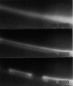
FIG. 1.: Experiment showing formation and instability of a collapsing bacterial cylinder (Reproduced from [7]). The first panel shows a diffuse cloud of bacteria filling the depth of a petri dish filled with agar, which then collapses (second panel) into a cylindrical structure. The cylinder subsequently destablizes into spherical aggregates. Details of the experiments are described in Budrene and Berg [5, 6].

Chemotaxis in E. coli is an excellent model system for studying singularity formation. The biochemical response of E. coli to a changing environment has been thoroughly characterized [8, 9, 10, 11, 12] over the past twenty-five years, so we understand how the bacteria sense and respond to their environment. As a consequence, it is possible to write down a “first principles” hydrodynamic theory for the motion of many bacteria [13, 14] in which the response coefficients are measurable. Quantitative comparison between theory and experiment is possible, and any discrepancies can be traced directly to the biochemistry of individual bacteria[7]. The application to singularity formation arose from the recent discovery by Budrene and Berg [5, 6] of an assay in which E. coli excrete aspartate, an amino acid which is also an attractant for nearby bacteria. Attractant diffusion drives aggregation because it leads to an effective force between individual bacteria: a higher density of bacteria in a given region leads to a higher attractant concentration, which then attracts more bacteria.

The initial interest in the Budrene-Berg experiment was stimulated by the symmetrical patterns that form when chemotactic bacteria are seeded in the center of a petri dish, as shown in their papers [5, 6].

Several theories have been developed for these patterns, most of which [15, 16, 17, 18, 19, 20] view the pattern formation as resulting from a linear instability of a (1 dimensional) travelling wave of bacteria. Recently, it was pointed out [7] that each of the aggregates in a a pattern corresponds to a density singularity in the hydrodynamic description of the bacteria. Therefore the pattern formation depends crucially on the dynamics of singularity formation. Singularities in chemotaxis were anticipated by Nanudjiah[21] and Childress and Percus[22] in studies of mathematical models of chemotaxis. An important feature, understood first by Childress and Percus, is that chemotactic collapse has a critical dimension: although collapse to an infinite density sheet is mathematically impossible, collapse to infinite density lines and points both can occur. It was argued in [7] that these facts crucially affect the patterns that can form .

In particular, Figure 1 shows a step in the formation of the aggregates. The initially diffuse band (filling the depth of agar) cannot form a singularity by collapsing only one of its dimensions to zero thickness; instead it collapses into a cylinder (contracting two of its dimensions simultaneously). The cylinder later destabilizes to form aggregates, for which all three dimensions contract simultaneously. Models [15, 16, 17, 18, 19, 20] viewing aggregate formation as the linear instability of a band cannot account for these experimental observations. These two different pictures of aggregates form lead to different conclusions about which biochemical parameters set the wavelength and structure of the patterns. For the “collapsing cylinder” mechanism advocated here, the characteristics of the pattern are set by the same biochemical cutoff which prevents an aggregate from reaching infinite density.

Cylindrical collapse is also important when a uniform density cloud of bacteria breaks into aggregates. Linear stability analysis of the uniform density state predicts that the cloud directly breaks down into spherical aggregates. However, experiments[23] find that the the clumping is hierarchical: the uniform density cloud first collapses as cylindrical structures which then break into spherical aggregates. An important unsolved question is to explain the geometry of the high density regions during collapse, and to predict the distribution of final aggregates.

In this paper, we use a combination of simulations and asymptotics to describe the breakdown of a cylinder in of three principal steps (Figure 2). First, the bacteria collapse as a cylinder towards a line of infinite density. In the second step, uniformity along the cylinder axis is broken, and a singularity develops at a single point. Finally, the remaining cylinder breaks up producing a sequence of spherical aggregates. Our primary conclusion connecting the present theory with the experiments is that the spacing between the aggregates in patterns such as Figure 2 is determined by the local depletion of chemicals which make aspartate production possible. According to Budrene[23], the most likely candidate for this is the overhead oxygen concentration in the cell. This prediction is qualitatively in accord with the experiments; moreover this parameter dependence could be directly tested in future experiments, and would serve to discriminate this theory from those based on pure linear stability analysis.

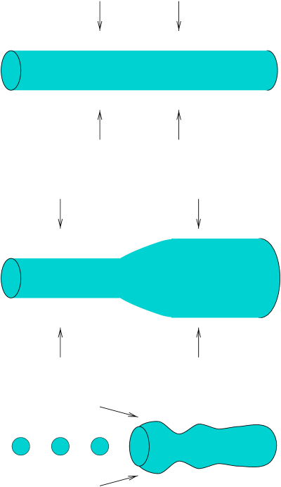
FIG. 2.: Schematic of the three phases of cylindrical collapse. Top, a collapsing cylinder is formed. Middle, the cylinder becomes modulated. Bottom, the modulated cylinder pinches off and contracts, leaving a series of spherical aggregates. Note this sketch does not show the radial contraction of the cylinder which takes place as it collapses.

In the following section, we review the basics of chemotaxis, and discuss details necessary to understand the Budrene-Berg experiments. Section 2 describes the cylindrical collapse of the bacteria. Cylindrical collapse (in which two dimensions of the cloud contract simultaneously) is a critical case [22, 24], for which diffusion and attraction nearly exactly balance. This criticality has complicated previous attempts to solve the collapse; a recent treatment of collapse in the 2D nonlinear Schrodinger equation [25] inspired our solution. In Section 3 we perform a stability analysis of a collapsing cylinder. Perturbations to the cylinder can be described by a “phase equation” for the singular time[26]. Solutions to this envelope equation explain full numerical simulations of a modulated cylinder. Section 4 describes the final stage of the breakdown of the cylinder, after the cylinder has pinched off at a point. Stability analysis predicts the breakup of the remaining column of bacteria, a situation analogous to a propagating Rayleigh instability in a liquid column[27]. Appendices describe our numerical methods, and fill in the details of the calculations.

I Problem Formulation: Bacterial Chemotaxis

Chemotaxis refers to the migration of bacteria up chemical gradients. For Escherichia coli, the basis of chemotaxis is largely understood [28, 29]: in the absence of a chemical gradient, an E. coli bacterium performs a random walk[30]. When chemical gradients are present, the bacterium’s internal biochemical reactions detect the gradients and couple to the bacterial movement system. This sensing biases the random walk, and the bacterium has a net drift towards a chemical attractant. Under special conditions, the bacteria can excrete the chemoattractant aspartate [5, 6] by converting carbon and nitrogen sources (succinate and ammonia, respectively) in their environment. In these experiments no external chemical gradients are present. Instead, each bacterium moves in response to the attractant produced by other bacteria. Thus, the excretion of attractant produces a long-range force between the bacteria, and induces complicated interactions in the colony.

The equations for the collective motion of the bacteria can be derived (with no free parameters) from the underlying biochemistry[14], allowing quantitative comparisons between theory and experiments. The basic equations for the bacterial density $\rho$ and the attractant concentration $c$ are

$$\frac{\partial\rho}{\partial t} = D_{b}\nabla^{2}\rho-\nabla\cdot\biggl{(}k\rho\nabla c\biggr{)}+a\rho$$ (1)

$$\frac{\partial c}{\partial t} = D_{c}\nabla^{2}c+\alpha\rho.$$ (2)

Here $D_{b}$ is the bacterial diffusion constant, $k$ the chemotactic coefficient, $a$ the rate of bacterial division, $\alpha$ the rate of attractant production, and $D_{c}$ the chemical diffusion constant. The terms in equation 1 include the diffusion of bacteria, chemotactactic drift and division of bacteria. Equation 2 expresses the diffusion and production of attractant.

Equations of this type were first used to describe bacteria by Keller and Segal [31], and, with variations, have been the subject of extensive investigations (see, e.g. [32, 33]). For E. coli, Schnitzer et. al. established the connection [13, 14] between the time averaged properties of the bacterial response and parameters in equations (1, 2). Thus, the extensive studies of individual bacteria provide a rigorous justification for the equations, as well as measurements of the coefficients. There is one complication to this statement that is worthwhile to mention: in 1975 Spudich and Koshland [34] showed that E. coli have “non-genetic individuality”, manifest in a distribution of tumble times (by about a factor of 2) between genetically identical bacteria. The consequence of this is that both time-averaged and ensemble-averaged properties of the bacteria are necessary to predict hydrodynamic coefficients; in addition, the dynamics must be such that the “distribution” of bacteria in the ensemble does not change with time.

It is convenient to nondimensionalize equations (1, 2) by choosing a characteristic density equal to the maximum initial density $\rho_{o}$. The characteristic scale of attractant is $D_{b}/k$. The density then determines the length scale and timescale according to $H=D_{b}D_{c}/(\alpha k\rho_{o})$ and $t_{o}=D_{c}/(\alpha k\rho_{o})$. Typical numerical values are $D_{b}=7\mbox{x}\>10^{-6}\mbox{cm}^{2}$/sec; $D_{c}=10^{-5}\mbox{cm}^{2}$/sec; $k=10^{-16}\mbox{cm}^{5}$/sec; and $\alpha=10^{3}$/second/bacteria. For an experiment [7] which has $\rho_{o}=10^{6}/\mbox{ cm}^{3}$, the length scale is 260 microns and the timescale 100 seconds. The equations become

$$\frac{\partial\rho}{\partial t} = \nabla^{2}\rho-\nabla\cdot(\rho\nabla c)+\delta\rho$$ (3)

$$\epsilon\>\frac{\partial c}{\partial t} = \nabla^{2}c+\rho,$$ (4)

where $\epsilon=D_{b}/D_{c}$ and $\delta=at_{o}$. For the experiments shown in Figure 1, cells divide much more slowly than the dynamics take place: the timescale for cell division is $\approx 2$ hours, giving $\delta\approx 0.01$. Therefore we approximate $\delta=0$. The value of the parameter $\epsilon$ varies: for experiments in semi-solid agar, the diffusion of bacteria is much slower than attractant diffusion, which motivates the limit $\epsilon=0$ [7]. For experiments on bacteria in a liquid culture, $\epsilon\approx 1$. We will consider both of these limits in this paper. The $\epsilon=0$ limit is particularly convenient for asymptotic calculations; we will use $\epsilon=0$ when doing analytic calculations. Our numerical simulations give results independent of $\epsilon$ in the range between 0 and 1.

For analytic calculations, working with the mass is particularly convenient, as will become apparent below. For reference, we show the form of the equations here. Define the mass contained within a radius $r$ as

$\displaystyle m(r)=\int dr\>r^{d-1}\rho.$This definition (and the limit $\epsilon=0$) allows us to eliminate the concentration and write the original equations as

$$\frac{\partial m}{\partial t}=r^{d-1}\frac{\partial\rho}{\partial r}+\rho m$$ (5)

II Cylindrical Collapse

In this section we construct the solution for a uniformly collapsing cylinder of bacteria, according to the evolution equations (3,4). Although the existence of cylindrical chemotactic collapse is well known [24], the asymptotic solution describing the collapse has never been constructed. Herrero and Velazquez [35] understood important features of two-dimensional collapse and attempted to find the solution; however, their solution is different from what we observe in numerical simulations (see Figure 4) and is therefore probably unstable.

The usual derivation of a similarity solution derives a set of ordinary differential equations from the scaling laws suggested by dimensional analysis. As shown below, the major difficulty arises because in the present situation these ODEs have no solutions consistent with the boundary conditions. This breakdown of “dimensional” scaling only occurs in two-dimensional collapse. In higher dimensions, the scaling laws suggested by dimensional analysis work fine [36]. The overall structure of this problem is similar to critical collapse in the focusing nonlinear Schrodinger equation [25], where the initial proposal for constructing the asymptotic solution involved rather intricate mathematics (continuation as a function of spatial dimension). Recently, a more physical derivation was put forward [25]. This work on the nonlinear Schrodinger equation inspired our construction of the solution for chemotactic collapse. Our central result is that the density singularity shows corrections to the dimensional scaling laws. Defining $\tau=t^{*}-t$ the distance to the singular time, the dimensional scaling law is $\rho=\tau^{-1}$. In the transient regime, we find a slow power law correction to this dimensional scaling law, $\rho\approx\tau^{-11/8}$. After the transient asymptotic regime, logarithmic corrections are present, of the form

$\displaystyle\rho=\frac{|\log|\log\tau||^{-1/2}}{\tau}.$Although the transient regime is present for 10 decades in the collapse time, we believe that this log log law is the asymptotically correct blow up rate. A log log correction also appears for 2D critical collapse in the nonlinear Schrodinger equation (See [25] and the references therein).

A Critical Dimension for Collapse

The competition between dissipation and collapse leads to a critical dimension. In this problem, the critical dimension is 2, and one dimensional collapse—that is, collapse to a planar structure with infinite density—is forbidden.

We make qualitative arguments to explain the critical dimension by comparing the chemotactic and diffusive fluxes in a contracting structure. First, no singularities exist for one-dimensional contraction. For a sheet of thickness $\ell$ the diffusive flux is of order (see equations (1, 2))

$$J_{\mbox{{D}}}\sim-D_{b}\frac{\rho}{\ell}.$$ (6)

The chemotactic flux follows by integrating $D_{c}c^{\prime\prime}\sim\alpha\rho$ and defining $M^{1D}$ as the mass per unit area of the planar region. Then the chemotactic flux is

$$J_{\mbox{{C}}}\sim k\rho c^{\prime}\sim\alpha k\rho M^{1D}D_{c}^{-1}.$$ (7)

If the system collapses onto a plane, the thickness of the sheet $\ell\to 0$. In this case the diffusive flux blows up while the chemotactic flux is unchanged. Thus a planar region with small thickness is unable to form infinite density, because diffusion eventually stops the collapse.

The situation is different for higher dimensional structures. For symmetric spherical collapse (three directions contract simultaneously), the chemotactic flux is singular. When we balance $D_{c}\nabla^{2}c\sim\alpha\rho$, we find $(r^{2}c^{\prime})^{\prime}\sim\alpha r^{2}\rho/D_{c}$. This implies a concentration gradient $c^{\prime}\sim\alpha M^{3D}/(\ell^{2}D_{c})$, where $M^{3D}$ is the mass contained within a radius $\ell$. The net inward flux of bacteria is then

$\displaystyle J\sim\frac{-D_{b}\rho}{\ell}+\frac{\alpha k\rho M^{3D}D_{c}^{-1}}{\ell^{2}}$As $\ell\to 0$ the inward flux (second term) dominates and collapse occurs.

In two dimensions we encounter a subtlety. Assuming cylindrical collapse and repeating the dimensional argument, we have $(rc^{\prime})^{\prime}\sim\alpha r\rho/D_{c}$, and $c^{\prime}\sim\alpha M^{2D}/(\ell D_{c})$. (Here $M^{2D}$ is the mass per unit length of the cylinder.) The inward flux is

$\displaystyle J=\frac{-D_{b}\rho+\alpha k\rho M^{2D}D_{c}^{-1}}{\ell}$Two dimensional collapse is critical: both fluxes have the same scaling with $\ell$. According to this simplified argument, there is a net inward flux if $M^{2D}>D_{c}D_{b}/(\alpha k)$, which suggests that a system with mass above this critical value collapses.

B Similarity Solutions

We now quantify the preceding dimensional arguments and collect the known solutions to the chemotactic equations. (As discussed above, the analytic solutions are derived with $\epsilon=0$.) First, consider one-dimensional collapse. Making the substitution[7] $v=\nabla c=\partial_{x}c$ in equations (3, 4) implies

$\displaystyle\frac{\partial v}{\partial t}=\frac{\partial^{2}v}{\partial x^{2}}-v\frac{\partial v}{\partial x}$This equation is the Burgers’ equation; singular solutions to this equation do not exist [37].

In $d=2$ and higher, density singularities can develop. In three dimensions, the nature of the blowup is straightforward. The characteristic length scale ($L$) varies in time, and the spatial structure is determined by the changes in $L$. A singularity corresponds to $L\rightarrow 0$. We guess the form of the similarity solution by balancing the different terms in equations (3,4). The diffusive dynamics imply $L=\sqrt{t^{*}-t}=\sqrt{\tau}$, with $t^{*}$ the singular time and $\tau$ the distance to the singular time. Defining a dimensionless similarity variable $\eta=r/L$, we find the scaling form of the density, concentration, and mass:

$$\rho = \frac{1}{L^{2}}R(\eta)$$

$$c = C(\eta)$$

$$m = L^{d-2}M(\eta)$$

In writing this form of solution, we have assumed radial collapse at the origin ($r=0)$. For a similarity solution to be valid, it must obey the correct boundary conditions: the density $\rho$ and the attractant concentration $c$ must be time-independent far from the singularity, which requires $R\sim\eta^{-2}$ and $C\sim$ constant as $\eta\to\infty$.

Plugging in the scaling form gives an ordinary differential equation in the similarity variable $\eta$. (Throughout this discussion, $d$ refers to the number of simultaneously contracting dimensions.)

$$\frac{\eta M^{\prime}}{2} = \eta^{d-1}R^{\prime}+RM$$ (8)

$$\eta^{d-1}R = M^{\prime}.$$ (9)

In $d=3$, the similarity equation can be solved exactly; the one stable solution, found by Kadanoff [36], is

$$R=\frac{4(3+\eta^{2})}{(1+\eta^{2})^{2}}$$ (10)

As demonstrated in [36], this solution well describes numerical solutions.

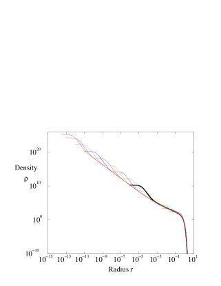
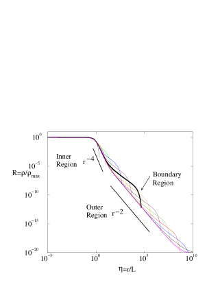
FIG. 3.: Density profiles for a collapsing cylinder. Different lines correspond to different times approaching the singularity. On the right, the density has been rescaled by the maximum density and the radius rescaled by the width. The solid line shows a profile at the same time both in this Figure and in Figure 8. The crossover between the stationary solution, for which the large $\eta$ behavior scales as $\eta^{-4}$ and the true outer solution, which scales is $\eta^{-2}$, is apparent.

C Solution in two dimensions

In two dimensions, there is no solution to equations (9,9) which satisfies the boundary conditions. To see this, note that the similarity equations can be integrated to give

$$R=e^{\frac{\eta^{2}}{4}}e^{\int\frac{M}{\eta}}$$ (11)

This form for $R$ cannot satisfy the boundary conditions that the density and mass be stationary at large $\eta$, because $R$ grows without bound as $\eta\rightarrow\infty.$

Nevertheless, a similarity-type solution to the equations exists, as Figure 3 shows. The density profiles at different times (left) have been collapsed by rescaling the length scale (right). This figure shows the basic features of the solution: in the “inner” region, there is a scaling solution. This matches onto an “outer” region far from the singularity, with a final “boundary” region where the boundary conditions must be satisfied. We illustrate this section with plots from a single numerical simulation. The numerical method is described in Appendix B; its most important feature is the remeshing, which moves mesh points every time the maximum density increases by one percent to better resolve the singularity [38].

How do we reconcile the numerical (and experimental) observations of two-dimensional collapse with the argument above that no solutions exist? We argue here that corrections to the similarity solution arise to solve this problem. We find in numerical simulations that although the basic self-similar scaling $\rho_{m}\sim L^{-2}$ is preserved, the time dependence of $L$ is different than the simple dimensional argument suggests. Figure 4 shows the scaling of $L$ with time: if the dimensional law $L\sim\sqrt{\tau}$ held, then $L/\sqrt{\tau}$ (plotted on the right) would be constant. Our simulations indicate a more complex time dependence than $L\sim\sqrt{\tau}$. We argue that the problem develops two timescales: a fast timescale on which collapse happens, and a slow timescale corresponding to changes in the similarity profile. Working in “similarity variables” allows a separation of these two timescales: we eliminate the known, fast time dependence so we can analyze the slow evolution of the system.

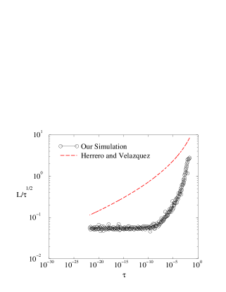
FIG. 4.: Time dependence of the length scale, $L$. In simulations, the length scale is defined as the length over which the density decreases by a factor of five, a characteristic of the inner region. The first plot shows $L$ versus distance to the singular time, which obeys close to a square root law. The second plot shows $L/\sqrt{\tau}$ versus $\tau$, showing evidence of the transient regime ($L/\sqrt{\tau}\sim\tau^{3/16})$ and, closer to the singularity, the asymptotic regime with logarithmic corrections to the length scale. For comparison, we have plotted the predictions of Herrero and Velazquez [35].

As $L\to 0$, the inner collapsing region converges to a similarity solution which we call the stationary solution because it has the same form as the stationary solution to the original equations. This asymptotic solution has a dimensionless mass of precisely 4. Thus, the evolution of the similarity solution has a specific physical interpretation. In dimensionless (similarity) variables, an inner region expels any excess mass to approach $M=4$. (Figure 5). Matching between the inner and outer regions determines the dynamics.

FIG. 5.: Schematic of cylindrical collapse.

1 Separation of Time Scales and Inner Solution

To find the solution, we use techniques originally applied to a similar problem in the 2D nonlinear Schrodinger equation[25]. We first define an important quantity: the collapse rate $A(t)=-\dot{L}L$. (Note that the collapse rate of the system is $\dot{L}/L$; we can make a dimensionless collapse rate by multiplying by the timescale $\tau\sim L^{2}$. Thus $A$ is the collapse rate.) For “regular” collapse, the collapse rate $-\dot{L}{L}=1/2$ is a constant. In the presence of corrections, the collapse rate goes asymptotically to zero.

We rewrite the similarity equation assuming that both quantities $M$ and $R$ depend on the similarity variable $\eta$ and (slowly) on time. The similarity equation is then

$$L^{2}\frac{\partial M}{\partial t}+A\eta M^{\prime} = \eta R^{\prime}+RM$$ (12)

$$\eta R = M^{\prime}.$$ (13)

Note that here the time derivative of $M$ refers only to explicit time dependence of the mass; the second term in the equation takes into account the time dependence slaved to the varying length scale.

We can solve the similarity equation in the inner region. As the collapse proceeds, it does indeed slow down. In fact, a numerical measurement of $A$ (Figure 6) shows that the collapse rate decreases by 3 orders of magnitude during the initial stages of the collapse. This motivates us to look for a solution with $A=0$; that is, a stationary solution (in similarity variables). This stationary solution solves Equations (12,13) when $A=0$ and $\partial_{t}M=0$. The equation for the mass is then

$\displaystyle\eta M^{\prime\prime}+M^{\prime}(M-1)=0.$Exact analytic solutions to this equation are

$$R_{o} = \frac{8}{(1+\eta^{2})^{2}}$$ (14)

$$M_{o} = \frac{4\eta^{2}}{1+\eta^{2}}$$ (15)

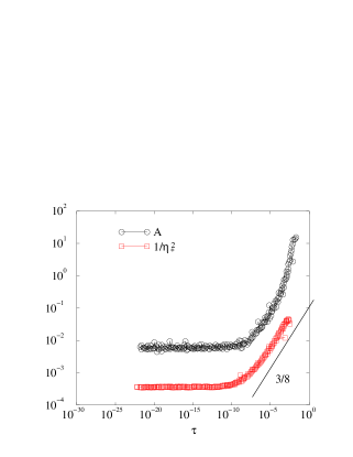
FIG. 6.: Plot of the collapse rate $A$ and $\eta_{*}^{-2}$ versus distance to the singular time $\tau$. The line shows a power law $A\sim\tau^{3/8}$. $A$ is measured by evaluating $\dot{L}L$ numerically; $\dot{L}$ is the difference in length scale between two time steps, divided by the time step size. The length scale $L$ is defined as the radial coordinate where the density decreases by a factor of 5. Similarly, $\eta_{*}$ is measured as the coordinate where the numerical density profile differs from the exact stationary solution (Equation (14)) by a factor of 4.

From the formula for $M_{o}$, we see an important feature of the stationary solution: the total mass is 4 in dimensionless units. This reflects a rigorous result[24, 36]: collapse will occur if and only if the total mass per unit length of the cylinder satisfies $M>4$. For $M<4$, no collapse is possible—the system evolves to constant density. For $M>4$, collapse occurs; however, numerical simulations show that the collapse converges toward a solution with a collapsing mass precisely equal to four. In similarity variables, therefore, mass flows away from the origin.

Compare this expression for $R_{o}$ to the numerical density profiles in Figure 3. The shape of the profile is accurately described by the formula for $R_{o}$, which confirms that the stationary solution holds in the inner region. At large $\eta$, the stationary solution has $R_{o}\sim 8\eta^{-4}$, while the boundary conditions require $R\sim c\eta^{-2}$. This “inner” solution to the equations must therefore match onto an “outer” solution, as shown in Figure 3. How to analyze this matching is the subject of the rest of this section.

Where does the crossover between inner and outer region occur? We can estimate the location of the crossover by noting that the crossover between inner and outer solutions will happen at some coordinate $\eta_{*}$, when $A\eta M^{\prime}\sim\eta R^{\prime}$ (see Equation (12)) This gives

$$\eta_{*}\sim A^{-1/2}.$$ (16)

The proportionality between $A$ and $\eta^{-2}_{*}$ is clear in numerics (Figure 6).

2 Transient Regime

Near the beginning of the collapse, the singular (inner) part of the solution has formed, but still strongly feels the influence of the boundary. During this initial, transient regime in the dynamics, excess mass is expelled. At the end of the transient regime, the true asymptotic state is reached. The transient regime is clear in the simulation shown here (Figures 4, 6, 9), where it persists until $\tau\approx 10^{-10}$. Here we attempt to analyze the transient regime and consider how the system approaches the asymptotic regime. This analysis is difficult, because the transient dynamics depend on the initial and boundary conditions of the system, and hence is particularly difficult to characterize analytically.

Why even bother with the transient behavior? Because, as we mentioned above, the transient regime persists until $\tau\approx 10^{-10}$. The density increases by 10 orders of magnitude before the true asymptotic dynamics are reached[39]. Therefore, all experiments can probe only the transient regime. Furthermore, the detailed dynamics of the transient regime are not highly sensitive to the initial conditions. We did a number of simulations in which the length scale of the initial density distribution was varied (Figure 7). When the density is initially almost constant, the time at which the singularity is reached, $t_{*}$, is large compared to a simulation in which the density is initially peaked. However, the transient dynamics are almost identical, regardless of whether the density is initially constant, or highly peaked [40].

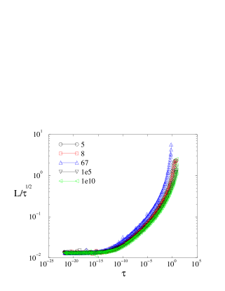
FIG. 7.: Comparison of different initial conditions. On the left, the time until the singularity is reached depends logarithmically on the length scale of initial density variation, as expected for an unstable collapsing mode. On the right, the transient regime dynamics are almost identical, despite the wide range in length scale of perturbation. The legend shows the length scale of initial density variation for each curve.

Our discussion of the transient regime that follows is incomplete and ad hoc. It is, however, the only self consistent explanation of numerical results we were able to find. We welcome additional, more conclusive work on this question.

We argue that the corrections to the length scale in the transient regime are faster than logarithmic. Although theoretically we cannot rule out logarithms, we were not able to find an asymptotic solution for a correction which depended purely logaritmically in time that explained all features of the numerical simulations. For this reason we believe that the most consistent interpretation of the transient regime is that it actually breaks the scaling laws predicted by dimensional analysis and introduces different exponents.

Here we use features of the numerical solution to guide our construction of the transient correction; this argument, while not entirely satisfactory, is at least consistent with all the simulations. We seek corrections to dimensional scaling of power law form: that is, $L\sim\sqrt{\tau}\tau^{\beta}$ and we are determining $\beta$. As long as $\beta>0$ , we still have asymptotic validity of the analysis, because $A$ goes to 0. (Note that $\beta$ depends on the initial and boundary conditions, and is not universal.)

We can distinguish between the transient and asymptotic regimes by looking at Figure 8. This plot shows profiles of the normalized density ($R(0)=1$) times $\eta^{2}$. At later times, the curve shows a flat region, demonstrating that $R\sim\eta^{-2}$ over a large region. This is the hallmark of the true asymptotic regime: the stationary solution is valid in the collapsing region, then $\eta^{-2}$ outer region exists far from the singularity, which in turn connects to the boundary. For earlier times, however, the flattened region is not present: instead the forming singularity connects directly to the outer “bump” where the excess mass has been pushed. [41]

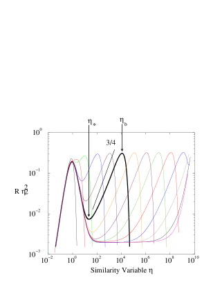
FIG. 8.: A plot of $R\eta^{2}$ versus $\eta$, used to construct the corrections in the transient regime. Profiles are for different times. The line shows a power law $\eta^{2}R\sim\eta^{3/4}.$ The heavy line shows the profile at the same time as the heavy line in Figure 3.

The inner solution must match on to the “bump” that makes up the outer region [42]. The bump corresponds to the excess mass in the system, which is stationary in real coordinates. Thus the position of the bump in similarity variables is $\eta_{b}\sim L^{-1}\sim\tau^{-1/2-\beta}$, where we have assumed power law corrections to the length scale. By reading off the plot (Figure 8) we can see two important features of the outer region: first, the value of $\eta^{2}R$ is constant at the position of the bump: $\eta_{b}^{2}R_{b}=\gamma$. Next, the form of the solution from the crossover point to the bump ($\eta_{*}<\eta<\eta_{b}$) is approximately a power law, which we write

$\displaystyle\eta^{2}R=c\eta^{\alpha}\mbox{ for }\eta_{*}<\eta<\eta_{b}$The exponent $\alpha$ is a free parameter that we find from the simulations. Taking $\alpha$ from the numerics (reading off Figure 8) uniquely determines all other scaling exponents and hence gives a consistency check. To determine $\beta$, combining the relations above lets us determine the time dependence $c\sim\eta_{b}^{-\alpha}\sim\tau^{\alpha(1/2+\beta)}$. This means that in the intermediate regime $\eta_{*}<\eta<\eta_{b}$ the solution obeys

$\displaystyle\eta^{2}R\sim\tau^{\alpha(1/2+\beta)}\eta^{\alpha}$Finally, we match the two solutions at the crossover $\eta_{*}$, leading to the result $\eta_{*}\sim\tau^{-\alpha(1/2+\beta)/(2+\alpha)}$. Demanding consistency in time scaling we must have $\eta_{*}^{-2}\sim A\sim\tau^{2\beta}$. This determines $\beta$:

$\displaystyle\beta=\frac{\alpha}{4}$For the simulations shown, $\alpha=3/4$. We have examined $\alpha$ for a variety of initial conditions and find it always to be close to this value. This one assumption for $\alpha$ leads to predictions for other measureable exponents, all of which are in good agreement with numerical simulations.

Thus in the transient regime we have

$$L = \sqrt{\tau}\tau^{3/16}$$

$$A = \tau^{3/8}$$

$$\rho_{m} = \frac{1}{\tau\tau^{3/8}}=\tau^{-11/8}$$

These scalings compare well with numerics, shown in Figures 4,6, and 9.

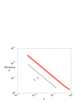
FIG. 9.: The scaling of the maximum density with time. On the left, $\rho_{m}$ versus $L$, which is well described by the expected scaling. On the right, $\rho_{m}\tau$ versus $\tau$, showing the transient and asymptotic regimes.

3 Asymptotic Regime

Once a true scale separation exists between the inner (collapsing) region and the boundary, the matching is different. Here we see slow (logarithmic) corrections in numerics, motivating us to seek a logarithmic correction to the length scale. We define the slow time scale $s=-\log\tau$, and seek a length scale $L$ of the form $L=\sqrt{\tau}/f(s)$. With this modification, Equations (12,13) for the mass becomes

$$\frac{1}{f(s)^{2}}\frac{\partial M}{\partial s}+A\eta M^{\prime}=\eta R^{\prime}+RM$$ (17)

The inner region must match onto an “outer” solution of the form $R=c\eta^{-2}$ The value of the coefficient $c$ can be estimated from the total mass and size of the system. If $c$ is independent of time, the total mass $M$ in the far field is logarithmically divergent: $M\sim c\log\eta$. However, conservation of mass requires that the total mass be constant at the boundary: $M(W)=M_{T}$, which implies $c\sim M_{T}/\log(W/L)$ (up to logarithmic corrections) or

$\displaystyle c\sim\frac{M_{T}}{\log W+s}.$As explained above, the crossover between inner and outer solutions occurs at $\eta_{*}\sim A^{-1/2}$. At $\eta_{*}$ we require that the mass flux $\partial M/\partial s$ is continuous; this condition connects the inner and other solutions, and fixes the dynamics of $f$.

From the similarity equation (17) and $R(\eta)=c\eta^{-2}$ we have the mass flux in the outer region

$$\frac{\partial M}{\partial s}=-Af^{2}c+O(\eta^{-2})\quad\eta\to\infty$$ (18)

The mass flux as $\eta\to\infty$ is spatially uniform. This must match the mass expelled by the inner region, which we find from $M_{o}\approx 4-\eta^{-2}$. Equating fluxes at $\eta_{*}$ gives $\partial M_{o}/\partial s|_{\eta_{*}}=-Af^{2}c$ or

$$\frac{\partial A}{\partial s}=Af^{2}c.$$ (19)

We can convert this to an equation for $f$ by using the definition of $A=-\dot{L}{L}=f^{-2}(1/2+f^{\prime}/f)\approx f^{-2}/2$, where a prime denotes derivative with respect to $s$. Plugging in the value of $c$ from above, we have an equation of the form

$\displaystyle\frac{-f^{\prime}}{f^{3}}=\frac{M_{T}}{\log W+s}$This relation holds for large $s$, giving the scaling of $f$ with time:

$\displaystyle\frac{-f^{\prime}}{f^{3}}\sim\frac{1}{s}$which gives

$\displaystyle f\sim\frac{1}{\sqrt{\log|\log\tau|}}$The asymptotic solution for two-dimensional collapse is a very slow ($\log\log\tau$) correction to the scaling laws from dimensional analysis. Our simulations cannot verify the functional form of $f$; however, we certainly see a crossover to slow (or nonexistent) corrections to the length scale. In Figures 4,6, and 9, the slow correction is visible for $\tau$ between $10^{-20}$ and $10^{-10}$. A blow-up of this slow correction show that it is approximately constant, but dominated by numerical noise—our numerics aren’t good enough to resolve this correction. Note that a simple logarithmic correction (that is, $f$ proportional to $\log\tau$) is not consistent with our simulation, because such a function would not be approximately constant over 10 orders of magnitude in time. Therefore, our numerics are consistent with, but not proof of, a log log correction.

III Evolution of a Modulated Cylinder

A collapsing cylinder eventually breaks into spherical aggregates. Here, we find the envelope equation which describes how modulations to the cylinder evolve. The challenge is to describe a collapsing cylinder. Collapse amplifies initially small perturbations; therefore small variations along the cylinder (in density and the radial length scale) become large. We can perform a valid perturbation analysis by studying variations in the singular time $t^{*}$.

In the original similarity solution, the singular time $t^{*}$ is undetermined: if $t^{*}$ changes by a constant, the solution remains valid. Allowing slow spatial variation in $t^{*}$ breaks this symmetry. Therefore we expect the variation of $t^{*}$ to produce slow dynamics in space and time. Because this mode is the most slowly decaying, it dominates the evolution of a cylinder. We derive a phase equation, an approach used in many problems when stability is governed by a slow mode associated with a broken symmetry[26]. Phase equations [43] were invented to understand problems like convection, where the relevant symmetry is translation, and the stability analysis is relative to a travelling wave solution. Earlier research moved towards applying phase equations to singularities: In previous work on blowup in the semilinear heat equation, Keller and Lowengrub [44] derived a transformation from a blowing-up variable to one that vanishes; they then perturbed in the vanishing variable. Also in the context of the semilinear heat equation, Bernoff [45] has looked at how the singular time varies along a cylinder.

We compare solutions of the phase equation to full numerics and show that the evolution of a modulated, collapsing cylinder is well described by the simplified phase equation.

A Derivation of a Phase Equation

This section gives a flavor of the derivation of the phase equation, for details see Appendix B. We seek an equation for the dynamics of $\tau(z,t)=t^{*}-t=t_{o}+T(z,t)-t$. Slow variation requires that both $T^{\prime\prime}\ll T^{\prime}$ and $\dot{T}\ll 1$. Once the collapse time varies along the axis of the cylinder, $R$ and $C$ are no longer exact solutions to the equations (3, 4). We write the correction as

$$R=R_{o}(\eta)+\delta R_{1}(\eta,z,t)$$

$$C=C_{o}(\eta)+\delta C_{1}(\eta,z,t)$$

where $\eta=r/L_{r}$, with the radial length scale $L_{r}=\sqrt{\tau(z,t)}/f(\tau)$, where $f$ is the correction to the length scale. The perturbation parameter $\delta$ is of order $L_{r}/L_{z}$, where $L_{z}$ is the scale of the density variation along the axis of the cylinder.

We insert this guess into the original equations, and expand in $\delta$. The lowest-order equation gives the original similarity equations. At first order, we find an equation of the form:

$$\Lambda(R_{1},C_{1})=F(R_{o},C_{o})(\tau_{t}+1)+G(R_{o},C_{o})\tau_{zz}+H(R_{o},C_{o})\frac{\tau_{z}^{2}}{\tau}$$ (20)

On the left side is a linear operator $\Lambda$ acting on $R_{1}$ and $C_{1}$; $\Lambda$ comes from the linearization of the original equations. The right hand side contains derivatives of the singular time multiplied by known functions of $R_{o}$ and $C_{o}$.

Although $R_{1}$ and $C_{1}$ are unknown, the right hand side is constrained by a solvability condition: Any function which is annihilated by the adjoint of $\Lambda$ must be orthogonal to the right hand side. That is, if $\Lambda^{\dagger}g=0$ for a nonzero $g$, then the inner product [46]

$\displaystyle\langle g,\Lambda(R_{1},C_{1})\rangle=\langle\Lambda^{\dagger}g,(R_{1},C_{1})\rangle=0.$Hence, the right hand side of (20) is orthogonal to $g$. In this case (see Appendix B) precisely one nonzero $g$ satisfies $\Lambda^{\dagger}=0$. Taking the inner products leads to a phase equation of the form

$\displaystyle c_{1}(\tau_{t}+1)+c_{2}\tau_{zz}+c_{3}\frac{\tau_{z}^{2}}{\tau}=0$where the constants $c_{1},c_{2},c_{3}$ can be expressed in terms of the known functions $g$, $F$, $G$, and $H$:

$$c_{1} = \langle g,F(R_{o},C_{o})\rangle$$

$$c_{2} = \langle g,G(R_{o},C_{o})\rangle$$

$$c_{3} = \langle g,H(R_{o},C_{o})\rangle$$

As shown in appendix B, for a cylinder disintegrating into spheres the phase equation is

$$\frac{\tau_{t}+1}{f^{2}}=\tau_{zz}-\frac{\tau_{z}^{2}}{\tau}$$ (21)

The correction terms in this equation arise directly from the corresponding corrections to the length scale in the similarity solution. In the subsequent section, we show that this results in asymptotically different scalings for the radial and axial length scales on the collapsing cylinder. (Hence, a “point” singularitity that forms on a collapsing cylinder does not have the same collapse rate as spherical collapse.) In the absence of corrections to dimensional scaling, the phase equation is simply

$$\tau_{t}+1=\tau_{zz}-\frac{\tau_{z}^{2}}{\tau}$$ (22)

B Numerical Simulations of a Collapsing Cylinder

Now we compare solutions to equation (21) with a fully nonlinear simulation of a collapsing cylinder. We have found two different mechanisms by which modulations of the cylinder can produce singularities: The first is a “point” singularity, in which the density blows up at a point on the cylinder; the second is a “travelling” singularity, which moves along the cylinder axis with a diverging velocity (as the singularity is reached.)

The primary technical difficulty in simulating a collapsing cylinder is developing a remeshing algorithm to closely approach the singularity. The meshing algorithm described here resolves density singularities along the axis of the cylinder with essentially arbitrary resolution. The algorithm is based on a simple one-dimensional scheme, which redistributes mesh points every $50$ timesteps to resolve the singularity. The two-dimensional algorithm uses the one-dimensional remeshing scheme along both $\hat{r}$ and $\hat{z}$ simultaneously; the two dimensional equations are then solved by operator splitting. Details of the algorithm are summarized in Appendix A.

A typical simulation [47] started with a $z$-independent initial condition, which was allowed to progress until the maximum density reached $10^{4}$. At this point, the radial profile of the collapse was well approximated by the (2-dimensional) collapsing similarity solution constructed in the previous section. We then added a $z$-dependent perturbation to the density profile, with amplitude much smaller than the ambient density.

The separation of scales hypothesis underlying the derivation of the phase equation is maintained uniformly in time. We experimented with different functional forms for the density perturbations; as long as the length scale $L_{z}$ for variation in the $z$ direction is longer than the variation in the radial direction $L_{r}$, perturbations tended to grow. In all cases, the relation $L_{z}\gg L_{r}$ was maintained. As demonstrated in Figure 10, a radial cross section of the cylinder always revealed density profiles in agreement with the two dimensional collapsing singular solution constructed in the previous section.

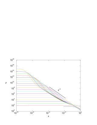
FIG. 10.: Figure showing the radial density profile at a single point on a modulated, collapsing cylinder. Note the $r^{-4}$ region matched onto the $r^{-2}$ region: The solution is well-described by the two-dimensional similarity solution throughout the collapse (cf. Figure 3) even in the presence of a $z$ dependent modulation.

Extensive simulations have found two types of density singularities caused by modulations to the cylinder.

1 Travelling Singularity

Travelling singularities occur when a step-like perturbation is placed on the cylinder, increasing the density for $z>z_{0}$ and decreasing the density for $z<z_{0}$. The subsequent evolution occurs at the boundary between these two regions. A simulation of this process is shown in Figure 11. The higher density region propagates to the left. Heuristically, the higher density region is beginning to contract as a sphere, so its decrease in size is consistent with the beginnings of spherical collapse.

This propagating singularity can be described as a solution to the phase equation of the form

$\displaystyle\tau=\tau_{o}\>\phi(z-z_{o}(t))$where $\tau_{o}=t^{*}-t$ is the basic phase expected from collapse. All the nontrivial space and time dependence is absorbed in $\phi$ and $z_{o}$. Inserting into the phase equation (21), we have

$\displaystyle\frac{\dot{\tau_{o}}\phi-\dot{z_{o}}\tau_{o}\phi^{\prime}+1}{f^{2}}=\tau_{o}\left(\phi^{\prime\prime}-\frac{\phi^{\prime 2}}{\phi}\right)$The right hand side of this equation is $O(\tau_{0})$, which becomes arbitrarily small as the singularity is approached. Therefore, the left hand side must be equal to zero, which gives

$\displaystyle\dot{\tau_{o}}\phi-\dot{z_{o}}\tau_{o}\phi^{\prime}+1=0.$If we demand the balance $\dot{z}_{0}\tau_{0}=-A$, then

$$z_{0}=A\log\tau_{0}.$$

The solution for $\phi$ is then

$\displaystyle\phi(\eta)=1+e^{\eta/A}.$

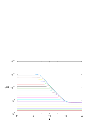
FIG. 11.: Time evolution of the centerline density $\rho(r=0,z)$, with a step function initial condition. The perturbation is seeded when $\rho=10^{4}$, and subsequent profiles show when the maximum density increases by a factor of five. The highest density region propagates to the left. Hence, the spatial extent of the high density region shrinks as the collapse is approached.

Figure 11 shows the density along the centerline of the cylinder. The decay of the highest density is exponential, as predicted by the phase-equation solution constructed above. A fit to the numerical data shows that

$$\rho(r=0,z)\sim e^{(-z/z_{0})}\sim e^{(-3.1z)}.$$

Figure 12 shows the location of the edge of the maximum density region $z_{0}(\tau)$ as a function of $\tau$. As predicted by the phase equation analysis, the figure shows that $z_{0}=A\log\tau$. A least squares regression gives the prefactor $A\approx 0.17$. The qualitative features of the numerical simulations are thus in good agreement with the theory. Quantitatively, however there is a discrepency: the theory predicts that we should have $A/z_{0}=1$, while our numerical simulation gives $A/z_{0}\approx 0.6$. We believe that the discrepancy arises because the convergence of our numerical scheme requires we keep a small $\epsilon\approx 0.1$, while the analysis in the previous subsection assumes $\epsilon=0$.

FIG. 12.: Location of the edge of the maximum density region $z_{0}(\tau)$ as a function of time. As predicted by the theory, the edge moves according to the law $z_{0}(\tau)=A\log\tau$. Regression gives $A\approx 0.17$.

2 Point Singularity

Stationary singularities—in which the blow-up happens at a spatial point—occur in the numerics for a wide variety of initial conditions. We believe that this represents the generic evolution of a modulated cylinder. Indeed, it is the end state of the travelling solution just discussed, when the propagating wave runs into the reflection–symmetric boundary condition. An instance of this solution is depicted in figure 13.

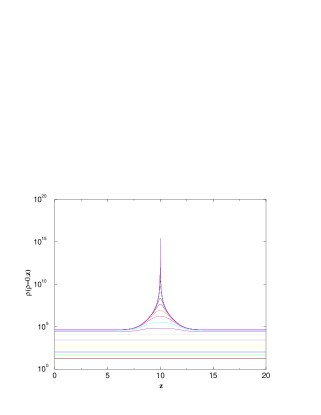
FIG. 13.: Time evolution of the centerline density $\rho(r=0,z)$, for a point singularity. The singularity was initiated by placing a perturbation (symmetric about $z=10$) on a uniformly collapsing cylindrical solution.

In contrast to the previous case, the corrections to dimensional scaling are important in this solution. For our analysis, we take the point of blow-up to be at $z=0$. Satisfying the equation requires that the $z$ length scale incorporate corrections to the scaling:

$\displaystyle\tau=\tau_{o}\phi\left(\frac{z}{\tau_{o}^{\beta}h(\tau)}\right)$Using $\xi=z/(\tau_{o}^{\gamma})$ the phase equation becomes

$\displaystyle f^{-2}\left(-\phi-\xi\phi^{\prime}(\gamma+\tau_{o}\frac{h^{\prime}}{h})\right)=\tau_{o}^{1-2\gamma}h^{-2}\left(\phi^{\prime\prime}-\frac{\phi^{\prime 2}}{\phi}\right)$Demanding that the two sides scale the same way in time (and assuming $h$ has a power law form, so that $\tau_{o}h^{\prime}/h=$constant), we have

$\displaystyle\frac{1}{f^{2}}=\frac{\tau_{o}^{1-2\gamma}}{h^{2}}$which gives $\gamma=1/2$ and $f=h$. Thus $L_{z}\sim\tau_{o}^{1/2}\tau_{o}^{-3/16}$, which differs from the radial length scale $L_{r}\sim\tau_{o}^{1/2}\tau_{o}^{3/16}$. The result is

$$\frac{L_{z}}{L_{r}}=\tau_{o}^{-3/8}$$ (23)

This shows that the generic density singularity that forms during the breakdown of cylindrical collapse, is not spherical collapse, but something milder. Locally, since the axial scale $L_{z}$ is much larger than the radial scale $L_{r}$ the structure still looks like a cylinder. Numerical evidence for this conclusion is evident in Fig 13, which shows that the singularity develops a length scale in the axial direction which is much larger than the radial scale $1/\sqrt{\rho}$. For example, in Fig 13 when $\rho=10^{10}$ (so $L_{r}=10^{-5}$) then $L_{z}\sim 10^{-2}$. Our numerical algorithms have unfortunately not allowed us to find the asymptotic $L_{z}/L_{r}$ numerically; the problem is that the separation of scales is so great between the radial and axial scales that one needs many more mesh points than we can afford to resolve the asymptotic regime.

IV Breakup into Spherical Aggregates

The question of relevance to the experiments is what happens next: Once blowup occurs at a spatial point the cylinder has a “free end”, which changes the nature of the collapse. We can no longer use the strategy of the previous section—perturbation about a collapsing cylinder—because the radial structure is no longer closely approximated by the cylindrical solution. The pinch-off drives the dynamics; specifically, the sharp end of the cylinder forms a travelling wave. Heuristically, note that an edge of bacteria produces a higher concentration of attractant where the density is higher. Thus the “tail” of bacteria moves toward higher attractant density, and a travelling wave can form. Quantitatively, recall that for variation in one spatial dimension the equations reduce to the Burgers’ equation, which has travelling wave solutions[37]. The contraction of a cylinder end has been observed for the bacteria [23], and the travelling waves have been discussed in other contexts[7]. Here we discuss the instability of the recoiling end and the final spacing of the spheres.

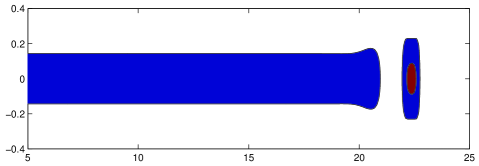
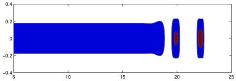
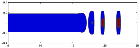
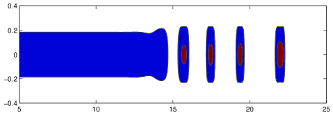
FIG. 14.: Numerical simulation of a collapsing cylinder with a free end, showing contour plots of the density. As the cylinder recoils, aggregates are left behind. The spacing between the aggregates is determined by the density of the cylinder as it collapse. The final frame in this figure shows the density profile along the centerline of the cylinder for the last contour plot (with 4 aggregates). Note the maximum density is near the cutoff density $\rho_{*}=500$ discussed in the text.

Figure 14 shows a set of numerical simulations of a retracting cylinder. The simulation shows that the “end” of the cylinder collapses into a spherical aggregate, and simultaneously, in front of the aggregate “waves” travel into the bulk of the cylinder. In the simulations, the ends of the cylinder actually try to collapse to an aggregate of infinite density. In order to continue beyond this singularity and simulate the formation of an array of aggregates we introduced a cutoff which emulates the biochemistry in the actual experiment: when the bacterial density becomes too high, the bacteria consume all the food sources (succinate and oxygen) in their local environment and cease producing the attractant aspartate. We modelled this by changing the equation for $c$ to

$\displaystyle\frac{\partial c}{\partial t}=D_{c}\nabla^{2}c+\alpha\rho\>e^{-\rho/\rho^{*}}$Here we have introduced $\rho^{*}$, the cutoff bacterial density. In [7] this cutoff density was estimated (assuming the cutoff was caused by oxygen depletion) and shown to vary exponentially with the overhead oxygen concentration in the cell: $\rho^{*}\sim e^{C_{Ox}}.$ For the simulation shown in Figure 14 this cutoff is $\rho^{*}=500$. Note that the density of the (undisturbed) cylinder in front of the retracting rim slowly approaches the cutoff density $\rho^{*}$; we have found in simulations that the undisturbed cylinder always collapses to a density close to the cutoff value.

The formation of the density wave occurs because the retracting end perturbs the cylinder in front of it. We can find the time-evolution of perturbations to the cylinder, requiring that they decay away from the free end. The most unstable mode can be found using methods of stationary phase(cf. [48]).

If the linear growth rate is $\omega(q)$ the point of stationary phase $q_{*}$ satisfies [48]

$$\mbox{ Im}\>\frac{d\omega}{dq}|_{q_{*}} = 0$$

$$\mbox{ Re}\>\frac{d\omega}{dq}|_{q_{*}} = \frac{\mbox{ Re}(\omega)}{\mbox{Im}(q)}$$

For the discussion here, we perform the calculation using the free space dispersion relation. A perturbation to constant density has the form

$$\rho = \rho_{o}+\delta e^{\omega t-qz}$$

$$c = \rho_{o}t+\chi e^{\omega t-qz}$$

where we have taken $\epsilon=1$ for simplicity in this calculation. Plugging into the equations and linearizing gives the dispersion relation:

$\displaystyle\omega=-i\sqrt{\rho_{0}}q+q^{2}$The most unstable mode is, in dimensionless units,

$$v_{*} = \sqrt{\rho_{0}}$$

$$q_{*} = \frac{\sqrt{\rho_{0}}}{2}(1\mp i)$$

$$\omega_{*} = \frac{\rho_{0}}{2}.$$

These formulae demonstrate that the wavelength of the modulations are governed by the undisturbed density in front of the rim. Since this density is asymptotically determined by the cutoff $\rho_{*}$, it follows that the wavelength of the ripples is determined by the cutoff. The characteristic distance between the aggregates is, therefore, determined by the cutoff. This conclusion can be experimentally tested.

The predictions for the wavelength and velocity of the front compare well with numerical simulations. On decreasing $\rho_{*}$ from $500$ to $140$ the wavelength of the ripples increases from $\approx 1.4$ to $2.5$, in qualitative agreement with the formulas.

We remark that the basic scenario outlined in this section was discovered by Elena Budrene, in unpublished experiments: After observing the travelling band to collapse as a cylinder (Fig. 1) Budrene observes fast “waves” propagating around the cylinder. Then, a fragmentation front moves across the collapsing cylinder, leaving spherical aggregates behind. The present theory predicts a scenario that is at least qualitatively very similar: the fast “waves” correspond to the excitations of the cylinder from the phase equation (i.e. the travelling steps, described in section 3). The fragmentation front occurs due to the mechanism outlined in this section. Unfortunately, it is not currently possible to make a quantitative comparison of the experiments to the present theory, though such a comparison would prove most interesting.

V Connection to Experiments

This paper has shown how the patterns formed by E. coli are connected to the geometry of singularity formation in the hydrodynamic description of the bacteria. We have constructed the solution for critical (two-dimensional) collapse, and developed a theory for modulations to the cylinder. The phase equation provides a useful simplified description of a perturbed cylinder. Ultimately, the spacing of spherical aggregates is determined by the instability of a pinched cylinder of bacteria.

Here we compare our work to published experiments and suggest tests of the theory. Not all the coefficients in the original equations have been precisely measured [7] for the experimental regime of interest. In particular, neither the attractant production rate $\alpha$ nor the chemotactic coefficient $k$ have been measured for bacteria in the same chemical environment as that of the collapse experiments. Thus, at this stage we can make only order of magnitude numerical comparison with experiments. Here we use the values of the coefficients for bacteria in a liquid medium [7]: bacterial diffusion coefficient $D_{b}=7\mbox{x}\ 10^{-6}\mbox{cm}^{2}$/sec; attractant diffusion coefficient $D_{b}=10^{-5}\mbox{cm}^{2}$/sec[49]; chemotactic coefficient $k=10^{-16}\mbox{cm}^{5}$/sec; and attractant production rate $\alpha=10^{3}$/second/bacteria

An important prediction of this theory is the critical mass of bacteria for cylindrical collapse: assuming the above parameters, the formation of a collapsing cylinder requires a minimum number of bacteria per unit length $M=4D_{b}D_{c}/(k\alpha)=3\mbox{x}10^{3}$/cm. The existence of a critical number of bacteria for cylindrical collapse has been inferred from experiments[7], but this number has never been directly measured. We emphasize that (with precise experimental measurements for the parameters $D_{b}$, $k$ and $\alpha$) the theory rigorously and precisely predicts this critical mass, allowing a direct test of the theory.

In this paper we have extensively discussed how to construct the correct description of two dimensional collapse. In the experiments, the subtle corrections to the dimensional scaling are probably not directly observable. However, the basic scaling relations expected from the similarity solution—for example, that the maximum density is related to the length scale of density variations by $\rho_{m}\sim L^{-2}$— could be measured in experiments, both for cylindrical and spherical collapse. So far, no quantitative and controlled measurements of the bacterial density have been performed.

In the section on cylindrical collapse, we discussed both the “transient” initial regime, and the final asymptotic regime which appears after true scale separation between the inner and outer solution is achieved. In practice, we expect that the experiments probe only the transient regime. The hard upper limit on bacterial density is when the bacteria are closely packed; this corresponds to a density of $2\mbox{x}10^{9}/\mbox{cm}^{3}$. A typical initial density of bacteria in the liquid experiments[7] is $10^{6}/\mbox{cm}^{3}$. The density increases by at most three orders of magnitude during the collapse, in contrast with the ten orders of magnitude it takes to reach the asymptotic regime in our simulations.

To our knowledge, modulations to a collapsing cylinder have never been quantitatively measured in experiments (although as mentioned above, Budrene has made qualitative observations of this effect). The travelling and point singularities that we predict for a modulated cylinder may be observable. In particular, we predict that the radial and axial length scales should be different for the point singularity. Because the difference in these length scales arises directly from the corrections in two-dimensional collapse, a measurement of these length scales would test the validity of our derivation of the two-dimensional solution.

The modulated cylinder ultimately pinches off a point. We have argued that the spacing of spherical aggregates is determined by the instability of a cylinder with an end. In practice, when does the modulated cylinder pinch off (forming an end)? To answer this question, we must know when our theory breaks down. Collapse to infinite density cannot happen for bacteria, because they have finite size. It was argued in [7] that even before the hard packing density of bacteria is reached, oxygen depletion will stop bacterial collapse. Regardless of the specific mechanism for stopping the collapse, at some time the highest density part of the cylinder—the point singularity—will stop collapsing. This is the time of pinch off: the point singularity evolves much more slowly than the neighboring, less dense regions of the cylinder.

This argument about the point of pinch off gives a testable prediction of our model, because the spacing of aggregates depends on the maximum density of the cylinder. In dimensional units, the most unstable wavelength (and aggregate spacing) is

$\displaystyle\lambda=4\pi\sqrt{\frac{D_{b}D_{c}}{\alpha k}}\rho_{m}^{-1/2}=300\mbox{cm}^{-1/2}\rho_{m}^{-1/2}$where we have used values of the coefficients from above. Thus, varying the maximum attainable density of the bacteria should cause the aggregate spacing to change according to this scaling law. In [7] a formula for how the maximum density in a collapsed aggregate depends on the oxygen concentration $C_{Ox}$ was derived, and shown to be $\rho_{m}\sim e^{C_{Ox}}$. This implies that the wavelength of the pattern should decrease exponentially with the oxygen concentration; systematic experiments could test this prediction.

The one solid prediction that can be compared with present experiments is that there is a lower bound on the aggregate spacing, that follows from the hard-packing density of bacteria. Using the characteristic size $10\mu$m of E. coli this is approximately $10^{9}/\mbox{cm}^{3}$. Thus the measured aggregate spacing should always be above the lower bound

$\displaystyle\lambda_{\mbox{min}}=0.1\mbox{ mm},$where in this estimate we used the assumed values for the constants $D_{b},k$ and $\alpha$. This lower bound agrees with experiments, in that the spacings are typically measured in millimeters.

Acknowledgements: We are grateful to Elena Budrene both for teaching us about her experiments that inspired this work and for many useful discussions. We acknowledge early discussions with Leonid Levitov, Leo Kadanoff and Shankar Venkataramani, and thank Daniel Fisher for helpful comments. This research was supported by the National Science Foundation Division of Mathematical Sciences, and the A. P. Sloan Foundation. MDB acknowledges support from the Program in Mathematics and Molecular Biology at the Florida State University, with funding from the Burroughs Wellcome Fund Interfaces Program.

A Remarks on Numerical Methods

The partial differential equations described in this paper were solved using second order in space, finite difference methods, supplemented with adaptive mesh refinement. The time discretization used a $\theta$ weighted Crank-Nicolson-type scheme (i.e. in the equation $\dot{f}={\bf L}f$ the right hand side is evaluated at time $(n+\theta)\Delta t$, where $\Delta t$ is the timestep). Typically, in the simulations with one spatial dimension, $\theta=0.6$. For the simulations in two spatial dimensions, we used an ADI operator splitting method, which requires using $\theta=1$. Because these methods are implicit, at each timestep a matrix inversion was necessary. This is the most expensive part of the numerical method.

The most subtle aspect of the numerical simulations reported in this paper is the mesh refinement. Without good mesh refinement it is impossible to get close enough to the singularity to resolve the (logarithmic) corrects uncovered for the cylindrical collapse; without good mesh refinement in the two-dimensional simulations it would be impossible to acquire enough decades of data to test the phase equation-theory presented in section 4. The mesh refinement was performed as follows:

One Spatial Dimension: The philosophy of mesh refinement employed in this paper (first explained to us by Jens Eggers) is to frequently implement gradual changes in the mesh, as opposed to infrequently implementing large changes. Mesh refinement is implemented every time the maximum density increases by one percent. During the refinement, the characteristic scale over which the solution varies is determined, and a mesh is constructed to well refine this scale; typically, this involves making sure there are about one hundred mesh points across the region that the solution varies significantly. The solution at the new mesh is constructed by cubic spline interpolation of the old mesh. Because the mesh is refined frequently, the changes to the solution occurring during refinement are small, and there are no convergence difficulties after refinement. The algorithm allows finding solutions over essentially arbitrary changes in the bacterial density with as little as few hundred mesh points. The simulations reported in the paper typically use a few thousand mesh points, in order to accurately compute the slow approach to the log log scaling regime.

Two Spatial Dimensions: In two dimensions, the equations are solved using standard operator splitting techniques. The mesh is rectangular, described by two functions, the $x$ coordinate $x_{i}$ and the $y$ coordinate $y_{j}$. Because the one dimensional algorithm described above can achieve arbitrary resolution with a few hundred mesh points, it is possible to well resolve density changes in both spatial directions using of order $10^{4}$ mesh points. The algorithm for these simulations works analogously to that for the one spatial dimension case described above: Every fifty time steps, the $x$ grid (or $y$ grid) is remeshed, in accordance with the criterea outlined above. Typically we stagger the remeshing between the two directions by twenty five timesteps.

Both the one and two dimensional codes were tested extensively by checking the solutions against known analytical results. All of the results that are presented in this paper follow the philosophy that numerical results are only believable if they can be replicated by asymptotic solutions of the equations; in turn, asymptotic results are only useful if they show up in numerics. For the two-dimensional code, one might worry that the operator splitting coupled with the remeshing induces artifical biases in the numerics; besides checking our numerical solutions against solutions to the phase equation, we have also tested the two dimensional code by checking that it can reproduce the scalings and the similarity solution for spherically symmetric collapse, where the solution is known very well.

B Phase Equation for a Bacterial Cylinder

In this section we fill in the details of the calculation of the phase equation. Evaluating the coefficients in equation (20) we find[50]

$$F(R_{o},C_{o}) = R_{o}+\frac{\eta R_{o}^{\prime}}{2}$$

$$G(R_{o},C_{o}) = R_{o}+\frac{\eta R_{o}^{\prime}}{2}-\frac{\eta R_{o}C_{o}^{\prime}}{2}$$

$$H(R_{o},C_{o}) = 2R_{o}+\frac{1}{4}(7\eta R_{o}^{\prime}+\eta^{2}R_{o}^{\prime\prime}-5\eta R_{o}C_{o}^{\prime}-\eta^{2}(R_{o}C_{o}^{\prime})^{\prime})$$

To evaluate the solvability condition, we need to find the zero mode of the adjoint to the linearized operator. In this case, the linear operator is the matrix

$\displaystyle\left(\begin{array}[]{cc}\nabla^{2}-\nabla\cdot(\nabla C_{o}\cdot)&-\nabla\cdot(R_{o}\cdot)\\ 1&\nabla^{2}\end{array}\right)$All of the terms in $\Lambda$ are self-adjoint except those of the form $\nabla\cdot(\nabla C_{o}\cdot)$. Under the definition (for a cylinder of bacteria) of the inner product $\langle f,g\rangle=\int rdr\int dzf^{*}g$ we can determine the adjoint

$\displaystyle[\nabla\cdot(\nabla C_{o}\cdot)]^{\dagger}=-\partial_{r}C_{o}\partial_{r}$which gives the adjoint linear operator

$\displaystyle\Lambda^{\dagger}=\left(\begin{array}[]{cc}\nabla^{2}+\nabla_{r}C_{o}\nabla_{r}&1\\ -\nabla\cdot(R_{o}\nabla\cdot)&\nabla^{2}\end{array}\right).$This linear operator possesses a simple zero mode: $\Lambda^{\dagger}(1,0)=0$. The coefficients of phase equation thus become

$$c_{1} = \langle 1,F(R_{o},C_{o})\rangle$$

$$c_{2} = \langle 1,G(R_{o},C_{o})\rangle$$

$$c_{3} = \langle 1,H(R_{o},C_{o})\rangle$$

A subtlety comes when we evaluate the inner products: we must integrate (in similarity variables) to the upper limit of validity of the similarity solution. For a cylinder, this upper limit is $\eta_{*}$, the radius at which the solution matches onto the outer solution. From the asymptotics discussed earlier, we use that $\eta_{*}\sim A^{-1/2}=f(s)$. Evaluating the inner products, and taking the limit $\tau\rightarrow 0$, we arrive at the result

$$c_{1} = \frac{-4}{f^{2}}$$

$$c_{2} = 4$$

$$c_{3} = -4$$

Which gives as the phase equation

$\displaystyle\frac{\tau_{t}+1}{f^{2}}=\tau_{zz}-\frac{\tau_{z}^{2}}{\tau}$

REFERENCES

- [1] Russel E. Caflisch and George C. Papanicolaou. Singularities in Fluids, Plasmas, and Optics, volume C404 of NATO ASI Series. Kluwer Academic Publishers, 1993.
- [2] A. Pumir and E. D. Siggia. Development of singular solutions to the axisymmetric Euler equati ons. Phys. Rev. Lett., 68:1511–1514, 1992.
- [3] J. Eggers. Universal pinching of 3d axisymmetric free–surface flow. Phys. Rev. Lett., 71:3458, 1993.
- [4] R. B. Larson. Numerical calculations of the dynamics of a collapsing protostar. Mon. Not. R. astr. Soc., 145:271–295, 1969.
- [5] E.O. Budrene and H.C. Berg. Complex patterns formed by motile cells of escherichia coli. Nature, 349:630–633, 1991.
- [6] E. O. Budrene and H.C. Berg. Dynamics of formation of symmetrical patterns by chemotactic bacteria. Nature, 376:49–53, 1995.
- [7] M. P. Brenner, L. Levitov, and E. O. Budrene. Physical mechanisms for chemotactic pattern formation by bacteria. Biophys. J., 74:1677–1693, 1995.
- [8] H. C. Berg and L. Turner. Chemotaxis of bacteria in glass capillary arrays. Biophys. J., 58:919–930, 1990.
- [9] A. J. Wolfe and H.C. Berg. Migration of bacteria in semi–solid agar. Proc. Natl. Acad.Sci. USA, 86:6973–6977, 1989.
- [10] S.M. Block and H. C. Berg. Successive incorporation of force-generating untis in the bacterial rotary motor. Nature, 309:470–472, 1984.
- [11] D. F. Blair and H. C. Berg. Restoration of torque in defective flageller motors. Science, 242:1678–1681, 1988.
- [12] J. E. Segall, S.M. Block, and H. C. Berg. Temporal comparisons in bacterial chemotaxis. Proc. Natl. Acad. Sci., 83:8987–8991, 1986.
- [13] M. J. Schnitzer, S. Block, H.C. Berg, and E. Purcell. Symp. Soc. Gen. Microbiol., 46:15, 1990.
- [14] Mark J. Schnitzer. Theory of continuum random walks and application to chemotaxis. Phys. Rev. E, 48:2553–2568, 1993.
- [15] R. Tyson. Pattern formation by e. coli–mathematical and numerical investigation of a biological phenomenon. 1996. Ph.D Thesis, University of Washington.
- [16] R. Tyson, S. R. Lubkin, and J. D. Murray. A minimal mechanism of bacterial pattern formation. Proc. R. Soc. Lond . B, 266:299–304, 1998.
- [17] E. Ben-Jacob, Inon Cohen, Ofer Shochet, I. Aranson, H. Levine, and L. Tsimring. Complex bacterial patterns. Nature, 373:566–567, 1995.
- [18] L. Tsimring, H. Levine, I. Aranson, E. Ben Jacob, I. Cohen, O. Shochet, and W. Reynolds. Aggregation patterns in stressed bacteria. Phys. Rev. Lett., 75:1859–1862, 1995.
- [19] D. E. Woodward, R. Tyson, M.R. Myerscough, J. D. Murray, E.O. Budrene, and H.C. Berg. Spatio-temporal patterns generated by salmonella. Biophys. J., 68:2181–2189, 1995.
- [20] W.J. Bruno. CNLS Newsletter, 82:1–10, 1992.
- [21] V. Nanjudiah. Chemotactaxis, signal relaying and aggregation morphology. J. Theor. Biol., 42:63–105, 1973.
- [22] S. Childress and J.K. Percus. Nonlinear aspects of chemotaxis. Math. Biosci., 56:217–237, 1981.
- [23] E. O. Budrene. Personal communication.
- [24] S. Childress. Chemotactic collapse in two dimensions. Lecture Note in Biomath., 55:61–68, 1984.
- [25] G. Fibich and G. Papanicolaou. Self-focusing in the perturbed and unperturbed nonlinear schroedinger equation in critical dimension, to appear in. SIAM Journal on Applied Mathematics, 1999.
- [26] P. Manneville. Dissipative Structures and Weak Turbulence. Academic Press, New York, 1990.
- [27] T. R. Powers, D. Zhang, R. E. Goldstein, and H. A. Stone. Propagation of a topological transition: The rayleigh instability. Phys. Fluids, pages 1052–57, 1998.
- [28] H. C. Berg. A physicist looks at bacterial chemotaxis. Cold Spring Harbor Symp. Quant. Biol., 53:1–9, 1988.
- [29] J. B. Stock and M. G. Surette. Chemotaxis. In Fredrick C. Neidardt, editor, Escherichia coli and Salmonella, pages 1103–1129. ASM Press, Washington, D.C., 1996.
- [30] H. C. Berg and D. A. Brown. Chemotaxis in escherichia coli analysed by three dimensional tracking. Nature, 239:500–504, 1972.
- [31] E.F. Keller and L.A. Segel. Initiation of slime mold aggregation viewed as an instability. J. Theor. Biol., 26:399–415, 1970.
- [32] J.D. Murray. Mathematical Biology. Springer Verlag, Berlin, 1989.
- [33] G.F. Oster and J. D. Murray. Pattern formation models and developmental constraints. J. Exp. Zool., 251:186–202, 1989.
- [34] J. Spudich and D. Koshland. Nongenetic individuality: chance in the single cell. Nature, 262:467–471, 1975.
- [35] M. A. Herrero and Juan J. L. Velazquez. Singularity patterns in a chemotaxis model. Math. Ann., 308:583–622, 1996.
- [36] M. P. Brenner, P. Constantin, L. P. Kadanoff, L. Levitov, A. Schenkel, and S. C. Venkataramani. Diffusion, attraction and collapse. 1999.
- [37] G. B. Whitham. Linear and Nonlinear Waves. Wiley and Sons, New York, 1974.
- [38] The simulation shown here used a box size with a total mass of and . For boundary conditions, we demanded reflection symmetry at the origin and zero flux at the outer boundary. Different initial conditions give similar final results; here we used a Gaussian profile.
- [39] In principle, the transient regime can be eliminated or shortened by preparing the system with mass very close to the critical mass . With less excess mass to expel, the system approaches the asymptotic state more quickly. However, even in simulations with the transient regime still persists for several decades. Since the density can increase by at most three or for orders of magnitude in experiments, the transient regime dominates the observed behavior.
- [40] This simulation used , mass , and . The characteristic length scale of the density distribution was varied, between 5 and , as shown in the Figure.
- [41] Here we note an interesting feature we observe in simulations: because the features of the transient regime are determined by matching to the boundary, the crossover time when the system reaches the true asymtotic regime varies with the system size. For a larger box size, the outer “bump” is farther away (in similarity variables) at a given time, and therefore the asymptotic regime is reached sooner.
- [42] Note that the presence of the bump reflects the boundary conditions applied in the simulation: we used no flux boundary conditions. As an example of a different boundary condition, requiring constant density at the boundary means the bump will not be present.
- [43] M. C. Cross and P. C. Hohenberg. Rev. Mod. Phys., 65:851, 1993.
- [44] Joseph B. Keller and John S. Lowengrub. Asymptotic and numerical results for blowing-up solutions to semilinear heat equations. In R. E. Caflisch and G. C. Papanicolaou, editors, Singularities in Fluids, Plasmas and Optics, pages 111–129. Kluwer, 1993.
- [45] A. J. Bernoff. Personal communication.
- [46] The inner product here is .
- [47] For the simulations presented in this section, the cylinder was represented on a mesh in , with boundary conditions that and , with a fixed constant ( in the simulations below). Reflection symmetry was enforced at both and , so that the solution is periodic in .
- [48] E. M. Lifshitz and L. P. Pitaevskii. Physical Kinetics, volume 10 of Course in Theoretical Physics. Pergamon Press, 1981.
- [49] Note that the estimate for the chemotactic coefficient given in [7] has an algebraic error.
- [50] The values of coefficients here were computed with for simplicity. When varies in time, there will be slight differences in th e numerical values of the coefficients; however these coefficients remain consta nt in time and the qualitative behavior of the phase equation is unchanged.