Abstract

We demonstrate that the information contained in the spike occurrence times of a population of neurons can be broken up into a series of terms, each of which reflect something about potential coding mechanisms. This is possible in the coding régime in which few spikes are emitted in the relevant time window.

This approach allows us to study the additional information contributed by spike timing beyond that present in the spike counts; to examine the contributions to the whole information of different statistical properties of spike trains, such as firing rates and correlation functions; and forms the basis for a new quantitative procedure for the analysis of simultaneous multiple neuron recordings. It also provides theoretical constraints upon neural coding strategies. We find a transition between two coding régimes, depending upon the size of the relevant observation timescale. For time windows shorter than the timescale of the stimulus-induced response fluctuations, there exists a spike count coding phase, where the purely temporal information is of third order in time. For time windows much longer than the characteristic timescale, there can be additional timing information of first order, leading to a temporal coding phase in which timing information may affect the instantaneous information rate.

In this new framework we study the relative contributions of the dynamic firing rate and correlation variables to the full temporal information; the interaction of signal and noise correlations in temporal coding; synergy between spikes and between cells; and the effect of refractoriness. We illustrate the utility of the technique by analysis of a few cells from the rat barrel cortex.

1 Introduction

Information about sensory stimulation is, at the most fundamental level, represented in the central nervous system by the spike emission times of populations of neurons. In principle, the temporal pattern of spikes across the neuronal population provides a large capacity for fast information transmission (?). It is still unclear how much of this theoretical capacity is actually exploited by the brain.

It has long been known that a substantial amount of sensory information is carried by the discharge rate of individual neurons (?). In some circumstances, however, if the stimulus is modulated on a very short time scale, precisely replicable sequences of spikes can be obtained (?; ?). Does this represent temporal coding, or is the relevant time window for counting spikes merely very short? Recent analyses have also suggested that temporally coded information is present in the spike trains of individual neurons in the monkey visual cortex under more general stimulation conditions (?; ?; ?). Evidence has also accrued that some information appears to be encoded by stimulus (or behaviour) related changes in the coordination of timing of firing between small populations of cortical cells (?, 1995; ?, 1996; ?, 1997). Given that our understanding of how spike trains are decoded biophysically is far from complete, the rigorous study of the information properties of nerve cells requires that we can quantify spike train information in full generality. Understanding neural coding then means understanding how the different features of the population of spike trains (such as spike counts, correlations or patterns) contribute to the full temporal information. This provides a powerful constraint upon the biophysical decoding that occurs: for instance, if no significant information about a stimulus is present in feature X of the spike trains, then none can be decoded by recipient neuronal pools by using ‘X detection’.

To study these questions, it is of interest to quantify information using a rigorous measure such as the mutual information (?; ?). In this context, the Shannon mutual information measures the extent to which observing a spike train (or a number of spike trains from several cells) reduces the uncertainty as to which external stimulus was present – it provides a bound upon well the stimuli can be discriminated. Equivalently, it measures the fidelity of coding on a trial by trial basis – how reproducibly the responses on individual trials represent the stimulus. If the spike times are observed with finite temporal precision $\Delta t$, and if $\Delta t$ is small enough such that all timing fluctuations below that timescale are not influenced by stimulation, then a binary string can be formed (with binwidth $\Delta t$) which contains all of the information present in the spike train. Direct estimation of the full temporal information is in principle possible by measuring the frequency of occurrence of all possible patterns of ones and zeros (‘words’) that the string can take from the experimental data (?; ?). A direct approach is particularly useful because it does not make any assumptions about what are the important aspects of the spike train, and is thus completely general. However, direct estimation by ‘brute-force’ estimation of frequencies is problematic, because of the large data sizes required (growing up to exponentially with wordlength). Despite this limitation, a recent study has succeeded in directly quantifying full temporal information from an alert animal, in part because of the low spiking rates obtained under the stimulation conditions used (?).

Another approach to direct calculation of the information is to expand the mutual information as a Taylor series in the experimental time window (?; ?; ?; ?). This is the approach taken here. In this paper we extend previous work based on the spike count response for a small population of cells (?) to present for the first time an analytical expression for the full temporal information in a population of spike trains to second order in the time window. This enables a natural separation of the contributions of both instantaneous firing rates and temporal correlations between spikes to the complete information. It also allows comparison with the information carried just by the number of spikes fired by each cell, which can be expressed in an equivalent form. This provides theoretical insight into the individual factors which determine the coding capabilities of neural spike trains. It also provides a procedure for neurophysiological data analysis which is superior with respect to data size requirements compared to ‘brute force’ frequency estimation of the information.

The use of such a Taylor series approach requires that the experimental time window (which should not be confused with the smaller binwidth used to discretise the spike train) be short enough that only a few spikes are emitted in its duration. This short time window limit, although a restriction, is relevant to the transmission of sensory information in the mammalian cortex. Single unit recording studies in primates have demonstrated that the majority of information about static visual stimuli is often transmitted in windows as short as 20-50ms (?; ?; ?). Information about time-dependent signals is often conveyed by single sensory cells by producing about one spike per characteristic time of stimulus variation (?). Event related potential studies of the human visual system (?) provide further evidence that the processing of information in a multiple stage neural system can be extremely rapid. The periods during which transcranial magnetic stimulation disrupts processing in early visual cortex have been found to be as short as 40 ms (?). Finally, the assessment of the information content of interacting assemblies which may last for only a few tens of milliseconds (?) requires the use of such short windows.

The paper is organised as follows: in section 2, the problem will be defined, and the series expansion of the information explained. In section 3, the necessary rate and correlation parameters will be introduced, and the probabilities of each possible response expressed in terms of these parameters. Section 4 gives the main result of the paper, the analytical expression obtained by substituting these probabilities back into the equation for mutual information. In section 5, we examine the conditions under which this approach is valid. Section 6 uses these results to study the role of response timescales in neural coding; two distinct coding régimes are found, depending upon the relative stimulus and response characteristic timescales. Temporal encoding may contribute significantly when the mean instantaneous firing rates of the cells fluctuate on a timescale shorter than the time window in which most of the information about the stimulus is transmitted. Section 7 examines the precision with which spike times may code information. In section 8, we study the conditions under which one finds synergistic relationships between spikes and between cells in an assembly. This includes an analysis of the effect of a refractory period on the spike train information. In section 9, we illustrate the method by applying it to spike trains recorded in the rat barrel cortex. Finally, in section 10, we discuss the consequences of the results and their relationship to other work.

2 The information carried by neural spike trains

Consider a time period of duration $T$, associated with a dynamic or static sensory stimulus, during which we observe the activity of $C$ cells. This period of physiological observation has associated with it a period (which might be earlier by some ‘lag’ time, but which we will consider to have the same length) in which we also observe the characteristics of an external correlate, such as a sensory stimulus, which might be influencing the cells’ behaviour. Let us denote each different stimulus history (time course of characteristics within $T$) as $s(\tau)$, a function of time from stimulus onset chosen from the set ${\cal S}$ of experimentally presented stimulus histories. We shall describe the neuronal population response to the stimulus by the collection of spike arrival times $\{t^{a}_{i}\}$, each $t^{a}_{i}$ being the time of occurrence of the $i$-th spike emitted by the $a$-th neuron.

Although the spike arrival time is a continuous variable, it can be experimentally measured only with finite precision $\Delta t$. Let us divide the time window $T$ into small bins of width $\Delta t$ (in which at most one spike per cell is observed). With complete generality, we can represent the spike sequence $\{t^{a}_{i}\}$ as a sequence of binary digits, one for each time bin and cell, with the response “1” in the bins corresponding to the spike times, and “0” in all other bins. We denote the probability of observing a spike sequence $\{t^{a}_{i}\}$ when a particular stimulus history $s(\tau)$ was present as $P(\{t^{a}_{i}\}|s(\tau))$ . $P(\{t^{a}_{i}\})=\left<P(\{t^{a}_{i}\}|s(\tau))\right>_{s}$ is its average across all stimulus histories. We determine $P(\{t^{a}_{i}\}|s(\tau))$ by repeating each stimulus history in exactly the same way on many trials, and observing the responses.

Following ?, we can write down the mutual information provided by the spike trains about the whole set of stimuli as

$$I(\{t_{i}^{a}\};{\cal S}) = \int{\cal D}s~{}p[s(\tau)]\int{\cal D}t_{i}^{a}p\left[\{t_{i}^{a}\}|s(\tau)\right]\log_{2}{p\left[\{t_{i}^{a}\}|s(\tau)\right]\over p(\{t_{i}^{a}\})}$$ (1)

$$\equiv \sum_{s(\tau)\in\cal S}P[s(\tau)]\sum_{t_{i}^{a}}P\left[\{t_{i}^{a}\}|s(\tau)\right]\log_{2}{P\left[\{t_{i}^{a}\}|s(\tau)\right]\over P(\{t_{i}^{a}\})}.$$

This notation can be read as follows. In the first, more general form of the equation, we use the functional integral notation $\int{\cal D}s$ to indicate that in principal, a continuous set of stimulus histories can be created. In practice, a discrete and often very limited set of stimuli is usually used to test the cell – hence we replace the functional integral with a summation over a discrete set of stimuli. For brevity, the $\tau$ will henceforth be dropped unless there is a particular need to stress the dynamic nature of the stimulus function. The notation $\int{\cal D}t_{i}^{a}$ indicates integration over all spike times $t_{i}^{a},i=1..n_{a},a=1..C$, and summation over all total spike counts from the population. $n_{a}$ is the number of spikes emitted by cell $a$. This notation is very similar to that utilised in (?, p. 158). In the limit of infinite precision, $\int{\cal D}t_{i}^{a}$ may be interpreted as a simple Riemannian integral; the results we present in this paper are valid in this continuous limit. More usually we will invoke finite precision $\Delta t$ and interpret the integral as a summation over all time bins.

In addition to studying the information contained in the sequence of spike times, we can also quantify the information contained in the response space defined by only the number of spikes emitted by each cell in the time window. We can form a $C$-dimensional vector ${\bf n}$, each component of which is $n_{a}$, the number of spikes fired by the respective neuron in the experimental time window. The spike count information can be written

$$I({\bf n};{\cal S})=\sum_{s\in\cal S}P(s)\sum_{{\bf n}}P({\bf n}|s)\log_{2}{P({\bf n}|s)\over P({\bf n})}.$$ (2)

This information quantity is exactly that calculated in (?). Invoking the data processing inequality, it is relatively obvious that $I({\bf n};{\cal S})\leq I(\{t_{i}^{a}\};{\cal S})$.

Now, the spike train information can be approximated by a power series

$$I(\{t_{i}^{a}\};{\cal S})=I_{t}(\{t_{i}^{a}\};{\cal S})\;T+I_{tt}(\{t_{i}^{a}\};{\cal S})\;{T^{2}\over 2}\;+\dots$$ (3)

where $I_{t}(\cdot)$ and $I_{tt}(\cdot)$ refer to the first and second time derivatives of the information respectively. As we shall see later, this becomes effectively an expansion in a dimensionless quantity, the number of spikes fired in the time window. For this approximation to be valid, the information function must be analytic in $T$, and the series must converge within a few terms. Both of these issues will be addressed in section 5. The time derivatives of the information can be calculated by taking advantage of the narrowness of the time windows, as will be explained.

3 Correlation functions and response probability

Before specifying the expressions for the response probabilities, it is necessary to define some response parameters. Consider first the discrete time resolution case (finite $\Delta t$). For each individual trial with stimulus $s$, the spike train density of each cell can be represented as a sum of pulses,

$$r_{a}(t;s)=\sum_{i}{\delta_{t,t_{i}^{a}}\over\Delta t},$$ (4)

where $\delta_{t_{1},t_{2}}$ is the Kroenecker delta function (1 if $t_{1}$ and $t_{2}$ label the same time bin, and zero otherwise). $i$ in the above indexes the spike number. The time-dependent firing rate is measured as the average of this quantity over all experimental trials with the same stimulus $s$. We denote this trial average by a bar, and the firing rate is thus $\overline{r}_{a}(t;s)$. Note that this mean rate function is sometimes called the post-stimulus time histogram, or PSTH.

It is also necessary to introduce parameters describing correlations among spikes. (Note that we use the word “correlation” to include both autocorrelation and crosscorrelation). Now, it is apparent that, for physically plausible processes, $\overline{r}$ will remain constant as $\Delta t\to 0$: if the mean firing rate is a differentiable function of time, then for sufficiently short bin widths, reducing $\Delta t$ will just reduce the probability of observing a spike accordingly. We would like to retain this property for our correlation measure as well, so that when we write out the series expansion of the information equation, there will not be any dependence upon time hidden inside the response parameters. Such hidden dependence would prevent a simple intuition of the dependence of the relative magnitudes of the information terms upon the timescale, and would, the authors, feel, be inelegant. The Pearson product moment, for instance, can be shown to approach zero for short time windows (?). The measure we choose is the scaled correlation density. We can write the scaled noise correlation density, which measures correlations in the response variability upon repeated trials of the same stimulus as

$$\gamma_{ab}(t^{a}_{i},t^{b}_{j};s) = \frac{\overline{r_{a}(t_{i}^{a};s)r_{b}(t_{j}^{b};s)}}{\overline{r}_{a}(t_{i}^{a};s)\overline{r}_{b}(t_{j}^{b};s)}-1,\;{\rm if}~{}a\neq b~{}{\rm or}~{}t_{i}^{a}\neq t_{j}^{b}$$

$$\gamma_{aa}(t^{a}_{i},t^{a}_{i};s) = -1.$$ (5)

The numerator of the first term indicates the average, over trials in which the same stimulus $s$ is presented, of the product of the spike densities of cell $a$ at time $t_{i}^{a}$ and cell $b$ at time $t_{j}^{b}$. Note that the scaled correlation density is simply a joint post-stimulus time histogram (JPSTH) from which the number of coincidences purely due to rate modulation has been subtracted (implemented by the “-1” in equation 5).

Now, we can introduce the above correlation parameters in terms of the conditional firing probabilities of observing one spike from cell $a$ in the time bin centered at $t^{a}_{i}$, given that cell $b$ emitted a spike in the time bin centered at $t^{b}_{j}$, when stimulus $s$ was presented:

$$P(t^{a}_{i}|t^{b}_{j};s)\equiv\overline{r}_{a}(t^{a}_{i};s)\;\Delta t[1+\gamma_{ab}(t^{a}_{i},t^{b}_{j};s)]+O(\Delta t^{2}).$$ (6)

This assumes that the conditional probabilities (6) scale proportionally to $\Delta t$. It is a natural assumption, as it merely implies that the probability of observing a spike in a time bin is proportional to the resolution $\Delta t$ of the measurement. It is violated only in the implausible and non-physical case of spikes locked to one another with infinite time precision. It can of course be checked for any given dataset; this will be carried out in section 5. Note that quadratic (and higher) order terms in $\Delta t$ were neglected from the above relationship as they affect only third and higher order terms of the information.

We will find it convenient to measure another type of correlation also: signal correlation, that is correlation in the mean responses of the neurons across the set of stimuli. These correlations can also be thought of as correlations in the tuning curves of the neurons. For homogeneity, we will also quantify these by a scaled correlation density:

$$\nu_{ab}(t^{a}_{i},t^{b}_{j})={\left<\overline{r}_{a}(t^{a}_{i};s)\overline{r}_{b}(t^{b}_{j};s)\right>_{s}\over\left<\overline{r}_{a}(t^{a}_{i};s)\right>_{s}\left<\overline{r}_{b}(t^{b}_{j};s)\right>_{s}}-1.$$ (7)

In the above, the brackets $\left<\cdot\right>_{s}$ can be taken to indicate the average across stimuli, $\int{\cal D}s~{}p(s)\cdot$ or $\sum_{s}P(s)\cdot$. Both $\gamma$ and $\nu$ may range from -1 to $\infty$, with zero indicating lack of correlation.

When passing to the high resolution limit ($\Delta t\to 0$), the same definitions outlined above apply, provided that we replace the Kronecker delta function with that of Dirac in the definition of spike density:

$$r_{a}(t;s)=\sum_{i}\delta(t-t_{i}^{a}),$$ (8)

and use probability densities instead of probabilities in equation 6.

Let us now consider the case of the spike count response parameters. The correlational parameters that influence the spike count information are the scaled correlation coefficients of the spike counts in each trial (?). These are obtained by summation over time bins (or integration in the high resolution limit) of the above expressions. The spike count scaled noise correlation coefficient can be written

$$\gamma_{ab}(s)={\int dt_{i}^{a}\int dt_{j}^{b}~{}\overline{r}_{a}(t_{i}^{a};s)\overline{r}_{b}(t_{j}^{b};s)[1+\gamma_{ab}(t^{a}_{i},t^{b}_{j},s)]\over[\int dt_{i}^{a}~{}\overline{r}_{a}(t_{i}^{a};s)][\int dt_{j}^{b}~{}\overline{r}_{b}(t_{j}^{b};s)]}-1.$$ (9)

Similarly, signal correlation is quantified as:

$$\nu_{ab}={\left<\int dt_{i}^{a}~{}\overline{r}_{a}(t^{a}_{i};s)\int dt_{j}^{b}~{}\overline{r}_{b}(t^{b}_{j};s)\right>_{s}\over\left<\int dt_{i}^{a}~{}\overline{r}_{a}(t^{a}_{i};s)\right>_{s}\left<\int dt_{j}^{b}~{}\overline{r}_{b}(t^{b}_{j};s)\right>_{s}}-1.$$ (10)

Equations 9,10 are a simple renotation of the definitions in (?) to fit with the requirements of the full temporal notation in the current paper. The finite resolution expressions for the above are of course obtained by replacing the integrals with summations:

$$\lim_{\Delta t\rightarrow 0}\sum_{n}f(t_{n})\Delta t=\int dtf(t)$$ (11)

If the conditional instantaneous firing rates are non-divergent, as assumed in equation 6, then the short time scale expansion of response probabilities becomes essentially an expansion in the total number of spikes emitted by the population in response to a stimulus. The only responses which contribute to the transmitted information up to order $k$ are the responses with up to $k$ spikes from the population. This is proved in Appendix A. The only relevant events for the second order analysis are therefore those with no more than two spikes emitted in total, and they can be truncated at second order without affecting the first two information derivatives. This is valid for any time-resolution. For brevity, we report the results only for the infinite time resolution case. The resulting expression (see Appendix A) is

$$P({\bf 0}|s) = 1-\;\sum_{a=1}^{C}\int dt_{1}^{a}\overline{r}_{a}(t_{1}^{a};s)+$$

$$+ {1\over 2}\sum_{a=1}^{C}\sum_{b=1}^{C}\int dt_{1}^{a}\int dt_{2}^{b}\overline{r}_{a}(t_{1}^{a};s)\overline{r}_{b}(t_{2}^{b};s)\left[1+\gamma_{ab}(t_{1}^{a},t_{2}^{b};s)\right]$$

$$p(t^{a}_{1}|s)dt^{a}_{1} = \overline{r}_{a}(t_{1}^{a};s)dt^{a}_{1}\left(1-\sum_{b=1}^{C}\int dt_{2}^{b}\overline{r}_{b}(t_{2}^{b};s)\left[1+\gamma_{ab}(t_{1}^{a},t_{2}^{b};s)\right]\right)\phantom{ppp}a=1,\cdots,C$$

$$p(t_{1}^{a}t_{2}^{b}|s)dt_{1}^{a}dt_{2}^{b} = {1\over 2}\overline{r}_{a}(t_{1}^{a};s)\overline{r}_{b}(t_{2}^{b};s)\left[1+\gamma_{ab}(t_{1}^{a},t_{2}^{b};s)\right]dt_{1}^{a}dt_{2}^{b}\phantom{ppp}a,b=1,\cdots,C;$$ (12)

where $P({\bf 0}|s)$ is the probability of zero response (no cells fire), $p(t^{a}_{1}|s)$ is the probability density of observing just one spike from cell $a$ at the specified time location, and $p(t_{1}^{a}t_{2}^{b}|s)$ is the probability density of observing just a pair of spikes at the given times.

4 Analytical results

We now insert the second order response probabilities (equation 12) into the expressions for the information contained in the sequence of spike times (equation 1) and the spike counts (equation 2). Then, for each term in the sum over responses, we utilise the power expansion of the logarithm as a function of $T$,

$$\log_{2}(1-T\;x)=-{1\over\ln 2}\sum_{j=1}^{\infty}{(Tx)^{j}\over j},$$ (13)

and, after integrating over spike times, group together all terms in the sum which have the same power of $T$. Equating these with equation 3 yields expressions for the information derivatives. These expressions depend only upon the time-dependent firing rates $\overline{r}$, the noise correlations $\gamma$, and the signal correlations $\nu$. As shown in Appendix A, the power expansion in the short time window length $T$ is related to the expansion in the total number of spikes emitted by the population. Therefore, although the formalism is for simplicity developed as an expansion in $T$, the expansion parameter is in fact the adimensional quantity representing the average number of spikes emitted by the population in the window $T$.

The first order contribution (i.e. $T$ times the instantaneous information rate) to the full temporal information from a population of spike trains is (?)

$$I_{t}(\{t_{i}^{a}\};{\cal S})\;T=\sum_{a=1}^{C}\int dt^{a}\left<\overline{r}_{a}(t^{a};s)\log_{2}{\overline{r}_{a}(t^{a};s)\over\left<\overline{r}_{a}(t^{a};s^{\prime})\right>_{s^{\prime}}}~{}\right>_{s}.$$ (14)

This is simply a sum of single cell contributions. It is insensitive to both signal and noise correlation.

The expression for the second order contribution (i.e. the second temporal derivative multiplied by $T^{2}/2$) breaks up into three terms:

$$I_{tt}(\{t_{i}^{a}\};{\cal S})\;{T^{2}\over 2} = {1\over 2\ln 2}\sum_{a=1}^{C}\sum_{b=1}^{C}\int dt_{1}^{a}\int dt_{2}^{b}\left<\overline{r}_{a}(t_{1}^{a};s)\right>_{s}\left<\overline{r}_{b}(t_{2}^{b};s)\right>_{s}$$ (15)

$$\times\biggl{\{}\nu_{ab}(t_{1}^{a},t_{2}^{b})+\left[1+\nu_{ab}(t_{1}^{a},t_{2}^{b})\right]\ln{1\over 1+\nu_{ab}(t_{1}^{a},t_{2}^{b})}\biggr{\}}$$

$$+ {1\over 2}\sum_{a=1}^{C}\sum_{b=1}^{C}\int dt_{1}^{a}\int dt_{2}^{b}\left<\overline{r}_{a}(t_{1}^{a};s)\overline{r}_{b}(t_{2}^{b};s)\gamma_{ab}(t_{1}^{a},t_{2}^{b};s)\right>_{s}\log_{2}{1\over 1+\nu_{ab}(t_{1}^{a},t_{2}^{b})}$$

$$+ {1\over 2}\sum_{a=1}^{C}\sum_{b=1}^{C}\int dt_{1}^{a}\int dt_{2}^{b}\biggl{<}\overline{r}_{a}(t_{1}^{a};s)\overline{r}_{b}(t_{2}^{b};s)\left[1+\gamma_{ab}(t_{1}^{a},t_{2}^{b};s)\right]$$

$$\times\log_{2}\biggl{\{}{\left<\overline{r}_{a}(t_{1}^{a};s^{\prime})\overline{r}_{b}(t_{2}^{b};s^{\prime})\right>_{s^{\prime}}\left[1+\gamma_{ab}(t_{1}^{a},t_{2}^{b};s)\right]\over\left<\overline{r}_{a}(t_{1}^{a};s^{\prime})\overline{r}_{b}(t_{2}^{b};s^{\prime})\left[1+\gamma_{ab}(t_{1}^{a},t_{2}^{b};s^{\prime})\right]\right>_{s^{\prime}}}\biggr{\}}\biggr{>}_{s}.$$

We will refer to these terms as components 2a, 2b and 2c of the information respectively.

When each spike is completely independent, as in a Poisson process, it is apparent that only the first term of equation 15 survives. It is easy to see that this term is always less than or equal to zero, since $f(x)=x-(1+x)\ln(1+x)$ has a global maximum at $f(0)=0$: the first term is equal to zero only if the signal correlation is precisely zero. This means that the information accumulation from a Poisson process with $|\nu|>0$ always slows down after the first spike.

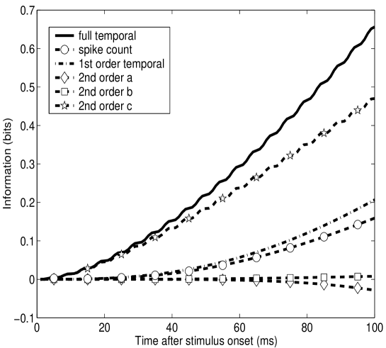
Figure 5: Panzeri, MS 2096

If there is any deviation from independence in the timing of successive spikes, then the other terms can contribute to the information through non-zero autocorrelation density $\gamma_{aa}(t_{1}^{a},t_{2}^{b})$. If there is any relationship between the times of spike emission of different cells, then they can contribute through non-zero cross-correlation $\gamma_{ab}(t_{1}^{a},t_{2}^{b})$. As with the spike count information terms detailed in (?), the second of these terms (the “stimulus-independent correlational component”) reflects contributions from a level of correlation which is not stimulus dependent. The third term is non-negative, and is non-zero only in the presence of stimulus dependence of the correlation between spikes, and is called the “stimulus-dependent correlational component”. The natural separation of the second order information into three components is important because each component reflects the contribution of a different relevant encoding mechanism. When applying this analysis to real neuronal data, a significant amount of information found in the third component of $I_{tt}$, relative to the total information, would clearly signal that cells are transmitting information mainly by participating in a stimulus (or context) dependent correlational assembly (?). A specific example will be given in Figure 5.

In the same way, the short time scale expansion can be carried out for the spike count information. This was performed in detail in ?, and here we report briefly the main results to cast them into identical notation to that above for comparison. The spike count information derivatives are similar to equation 15, but they depend only on the mean rate across time and on the spike count correlation coefficients (9,10). The first order contribution is:

$$I_{t}({\bf n};{\cal S})\;T=\sum_{a=1}^{C}\left<\int dt^{a}\overline{r}_{a}(t^{a};s)\log_{2}{\int dt^{a}\overline{r}_{a}(t^{a};s)\over\left<\int dt^{a}\overline{r}_{a}(t^{a};s^{\prime})\right>_{s^{\prime}}}~{}\right>_{s}$$ (16)

As before, the second order contribution is broken into three components:

$$I_{tt}({\bf n};{\cal S})\;{T^{2}\over 2} = {1\over 2\ln 2}\sum_{a=1}^{C}\sum_{b=1}^{C}\left<\int dt_{1}^{a}\overline{r}_{a}(t_{1}^{a};s)\right>_{s}\left<\int dt_{2}^{b}\overline{r}_{b}(t_{2}^{b};s)\right>_{s}$$ (17)

$$\times \biggl{[}\nu_{ab}+(1+\nu_{ab})\ln{1\over 1+\nu_{ab}}\biggr{]}$$

$$+ {1\over 2}\sum_{a=1}^{C}\sum_{b=1}^{C}\left<\left(\int dt_{1}^{a}\overline{r}_{a}(t_{1}^{a};s)\right)\left(\int dt_{2}^{b}\overline{r}_{b}(t_{2}^{b};s)\right)\gamma_{ab}(s)\right>_{s}\log_{2}{1\over 1+\nu_{ab}}$$

$$+ {1\over 2}\sum_{a=1}^{C}\sum_{b=1}^{C}\biggl{<}\left(\int dt_{1}^{a}\overline{r}_{a}(t_{1}^{a};s)\right)\left(\int dt_{2}^{b}\overline{r}_{b}(t_{2}^{b};s)\right)\left[1+\gamma_{ab}(s)\right]$$

$$\times \log_{2}\biggl{\{}{\left<\int dt_{1}^{a}\overline{r}_{a}(t_{1}^{a};s^{\prime})\int dt_{2}^{b}\overline{r}_{b}(t_{2}^{b};s^{\prime})\right>_{s^{\prime}}\left[1+\gamma_{ab}(s)\right]\over\left<\int dt_{1}^{a}\overline{r}_{a}(t_{1}^{a};s^{\prime})\int dt_{2}^{b}\overline{r}_{b}(t_{2}^{b};s^{\prime})\left[1+\gamma_{ab}(s^{\prime})\right]\right>_{s^{\prime}}}\biggr{\}}\biggr{>}_{s}.$$

5 Limitations

In this section we address the potential limitations of the technique presented here as a procedure for the analysis of real data. There are four assumptions which must be satisfied for the series approximation to be guaranteed to be a good estimate of the true information. These are: that the experimental time window is small; that the conditional firing probability scales with $\Delta t$; that the information is an analytic function of time; and that experimental trials are statistically indistinguishable.

Assumption 1. The short time scale limit utilized here formally requires that the mean number of spikes in the time window be small. The actual range of validity of the order $T^{2}$ approximation will depend on how well the time dependence of the information from the neuronal population fits a quadratic approximation. The range of validity for the spike count series information was checked by simulation in (?). The same range of validity must hold for the temporal information as well when the firing rates and correlations of the neurons vary slowly with respect to the time window considered, since in this limit the additional temporal information is small (see next section). The additional numerical test required here is therefore on the range of applicability of the second order approximation for the full spike timing information when the parameters describing the neuronal firing probabilities fluctuate quite rapidly within the time window $T$.

For this purpose we simulated neurons driven by two stimuli. The response of each neuron to each stimulus was modeled as a 1 ms resolution Poisson process with a time dependent firing rate (the response in each 1 ms time bin is generated with a time dependent firing rate independently of the response in the other time bins). The first stimulus gave a constant (flat) mean response $r_{0}=30$ spikes/sec. across time, whereas the second stimulus was chosen to produce a response of mean $r_{0}$ and sinusoidally modulated with amplitude $r_{0}$, at a frequency $1/\tau_{c}$. After a full period, the two stimuli are indistinguishable on the basis of spike count alone, and therefore this is a good model for examining temporal coding.

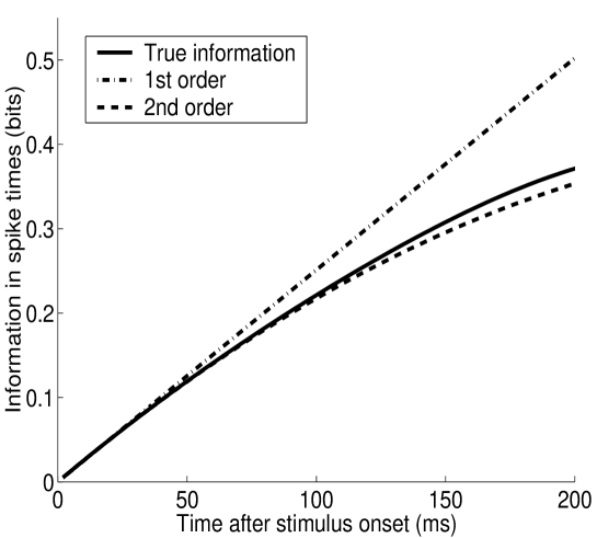
Figure 1: Panzeri, MS 2096

The analytical approximations to the information were tested against the true information computed directly from the model response probabilities. Figure  1 shows the accuracy of the first and second order approximations to the information in the spike times for a single cell with responses to the second stimulus oscillating very fast (at a frequency of 500 Hz). The second order approximation is nearly exact up to 200 ms, even in the extreme case of such fast fluctuations. The range of validity seems not to be significantly affected by changing the frequency of oscillations. We have also carried out simulations with a set of two cells with either Poisson or cross-correlated firing. When simulating two cells, we could not systematically test time windows as long as 200 ms because the number of spike trains over which we have to sum to compute the full information increases exponentially both with the length of the window and with the population size. However, we found that the scaling expectation that the range of validity shrinks as $1/C$ with population size is confirmed up to the time window lengths that we could test.

The simulations presented here therefore show that the series expansion can useful for time scales relevant to neuronal coding, for the small ensembles of cells typically recorded during in vivo experimental sessions. In particular, when correlations between spikes are weak the series expansion is very precise up to hundreds of ms. However, one should be aware that the presence of very strong correlations between the spikes can potentially reduce this range of validity. Therefore the actual range of validity for the data under analysis should be further assessed by looking e.g. at the agreement between the series expansion result for spike counts and the brute force evaluation of the spike count information from response probabilities (equation 2). (The latter, unlike the brute force full temporal information, can usually be computed with an experimentally feasible number of trials). An example of this check is given in section 9.

Assumption 2. The second assumption required is that the probability of observing a spike in the time bin centered upon $t_{i}^{a}$ from cell $a$ given that one has been observed in the time bin centred upon $t_{j}^{b}$ from cell b scales with $\Delta t$. This is captured by equation 6. This assumption would be expected to break down only if there were a significant number of spikes synchronised with near-infinite precision.

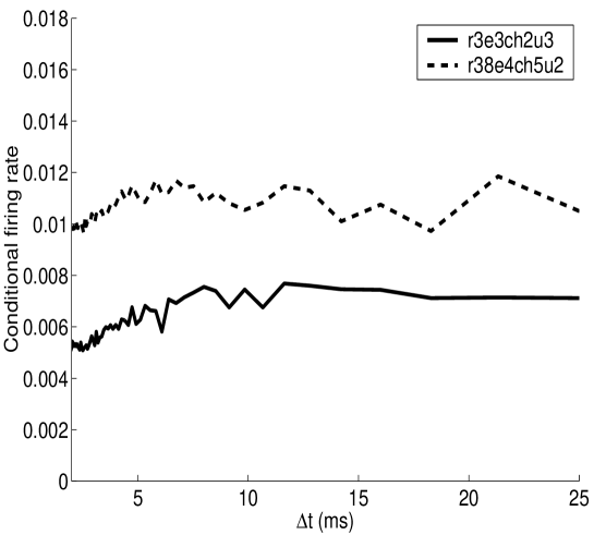
Figure 2: Panzeri, MS 2096

To illustrate how this scaling assumption can be validated experimentally, we examined the scaling relation between the average value of $P(t^{a}_{i}|t^{b}_{j};s)$ and $\Delta t$ for two neurons recorded from the rat barrel cortex. The stimuli were upward deflections of one of 9 whiskers. This data was provided by M.E. Diamond and colleagues. For further reference to the data see (?) and section 9, were the information properties of the same two cells are analyzed with our method. The result can be seen in Figure 2. We found that the averaged conditional firing rate, computed as the average across all bin pairs and stimuli of $P(t^{a}_{i}|t^{b}_{j};s)/\Delta t$, remained approximately constant as $\Delta t$ was decreased, and no divergence of the conditional firing rate was observed for all the resolutions considered. This provides evidence that Assumption 2 holds for this dataset.

Assumption 3. This method expands the mutual information as a Taylor series in $T$. Therefore the third required assumption is that the information is an analytic function of the time window size $T$. This requirement ensures that the Taylor series expansion of the mutual information exists, and that the series converges to the mutual information.

The validity of this assumption can be tested, at least to some extent, on the dataset under analysis. For example, one can check that there are no discontinuities in time of the firing parameters. Also, if there are enough data, the mutual information can be computed by brute force from the Shannon formula, equation 1, although it can be usually computed only for a more limited time range than when using the series expansion (see section 9). Hence the information computed by brute force from the Shannon formula can be compared, in some time windows, to the series expansion estimation. This provides a strong check of the validity of this particular assumption and of the convergence of the series expansion method, as fully illustrated in section 9. It is apparent that the assumption is valid for the data we examined here (see section 9). This assumption is more likely to cause problems with artificially constructed models implementing instantaneous correlations between neurons. One could argue that such models are non-physical in any case.

Assumption 4. The final assumption required is that experimental trials are statistically indistinguishable. This assumption is of course inherent to any neurophysiological data analysis, and is taken to be the definition of an experimental trial. Satisfaction of this assumption is the domain of experimental design.

6 Response timescales and pure temporal coding

Having quantified the information $I(\{t_{i}^{a}\};{\cal S})$ in the spike times and $I({\bf n};{\cal S})$ in the spike counts as a function of the rates and correlations, we are in a position to study the conditions under which information is not dominated by the spike counts. In other words, we ask: how much extra information, not contained in the spike counts, is conveyed by the temporal relations between spikes. This extra information is precisely $I(\{t_{i}^{a}\};{\cal S})-I({\bf n};{\cal S})$.

We find that the crucial parameter is the typical timescale of variation of the firing rate and correlation functions, relative to the time window $T$ of interest. We will label this typical or characteristic stimulus-induced response timescale $\tau_{c}$.

Case 1, large $\tau_{c}$. If the scale of time variation of any time dependent function $f(t)$ is large compared to the time window considered, then $f(t)$ can be approximated by its power expansion and the following quasi-static approximation holds:

$$\int_{t_{0}-T/2}^{t_{0}+T/2}f(t)dt=f(t_{0})\;T+{\partial^{2}\over\partial t^{2}}f(t)|_{t=t_{0}}\;{T^{3}\over 24}+O(T^{5})$$ (18)

As a consequence, if both rate and correlation functions vary slowly in the time domain of interest, only the rate and correlation values near the centre of the interval ($t_{0}$) are important, and the extra amount of information in the spike times is sub-leading (only of order $T^{3}$). The expression for the $T^{3}$ term in the extra information in spike timing can be computed by applying equation 18) to the integrals over time involved in computing information rates (equations 14 and 16). The result depends only on the firing rate variations near $t_{0}$, and not on correlations between the spikes.

$$I(\{t_{i}^{a}\};{\cal S})-I({\bf n};{\cal S})=$$

$${T^{3}\over 24\ln 2}\sum_{s}P(s){\partial\over\partial t}r(t;s)|_{t=t_{0}}$$

$$\left({(\partial/\partial t)r(t;s)|_{t=t_{0}}\over r(t_{0};s)}-{<(\partial/\partial t)r(t;s^{\prime})|_{t=t_{0}}>_{s^{\prime}}\over<r(t_{0};s^{\prime})>_{s^{\prime}}}\right).$$ (19)

(19) can be shown to be non-negative for any rate function, as required by information theoretical consistency.

Being of order $T^{3}$, in this régime pure temporal coding affects neither the rate nor acceleration of information transmission. Pure temporal information would accumulate very slowly with time. Therefore under these circumstances information is dominated by the spike counts.

Case 2, small $\tau_{c}$. If either firing rates or correlation functions fluctuate with a characteristic timescale smaller than $T$, then the quasi-static approximation (18) breaks down, and there is a transition to a different coding régime. A possible case may be the presence of a sinusoidal component of period shorter than $T$ in the rate fluctuations. If in particular $\tau_{c}$ is much shorter than $T$, the integral of the function over the time window does not depend on the value of the function at the center of the interval as in equation 18, or on the frequency of response variations, but only on the average value of the function over the period $\tau_{c}$:

$$\int_{t_{0}-T/2}^{t_{0}+T/2}f(t)dt=\left[{1\over\tau_{c}}\int_{\tau_{c}}f(t)dt\right]\;T\;+O(T^{2})$$ (20)

As a consequence, in this limit the additional purely temporal information is proportional to $T$ (and not to $T^{3}$ as in the quasistatic phase):

$$I(\{t_{i}^{a}\};{\cal S})-I({\bf n};{\cal S}) = \sum_{a=1}^{C}\int dt^{a}\left<\overline{r}_{a}(t^{a};s)\log_{2}{\overline{r}_{a}(t^{a};s)\over\left<\overline{r}_{a}(t^{a};s^{\prime})\right>_{s^{\prime}}}~{}\right>_{s}$$ (21)

$$- \sum_{a=1}^{C}\left<\int dt^{a}\overline{r}_{a}(t^{a};s)\log_{2}{\int dt^{a}\overline{r}_{a}(t^{a};s)\over\left<\int dt^{a}\overline{r}_{a}(t^{a};s^{\prime})\right>_{s^{\prime}}}~{}\right>_{s}$$

$$+ O(T^{2})$$

This means that when rates fluctuate rapidly the actual rate of information transmission (measured in bits/sec) can be considerably faster than that with spike counts only. Thus in this phase there can be substantial pure temporal information, and it may even be dominant with respect to the spike count information.

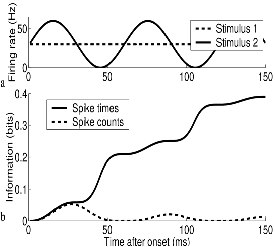
Figure 3: Panzeri, MS 2096

We studied particular cases by simulating mean firing rate and correlation parameters for each timestep as described in section 5. Two stimuli were again used, once inducing a flat rate response function, and the second a sinusoidally modulated function of time. The following results were obtained with 1 ms time resolution, but have also been confirmed by numerical integration in the infinite time-resolution limit. The effect of timing precision is considered separately. Figure 3 illustrates a situation in which the spike count of a single cell responding according to a Poisson process is unable to discriminate between the stimuli after a full period, but such information is available from spike timing. The time window is increased, beginning at the onset of stimulus-related responses. In this case, after 60 ms (a full cycle of oscillation), the spike count information drops to zero, whereas the full temporal information accumulates cycle after cycle. After one cycle the information is purely temporal.

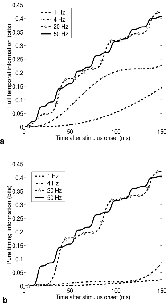
Figure 4: Panzeri, MS 2096

The effect of stimulus modulation frequency on the full temporal information is shown in Figure 4a. Figure 4b shows the purely temporal information for the same situation (i.e. the full information minus the spike count information). The difference between the fast and slow régimes can be seen by comparing these two figures. Slow fluctuations lead to negligible (of order $T^{3}$) pure temporal information. In the fast regime, pure temporal information increases roughly proportionally to the window length. Note also that, if fluctuations are very fast ($\tau_{c}\ll T$) and the spike incidence is measured with high temporal precision, the amount of information is roughly independent of the frequency of oscillation, as predicted by (20).

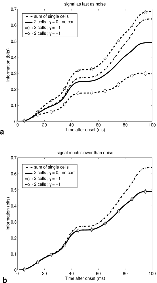
Figure 7: Panzeri, MS 2096

If the rates vary slowly with respect to $T$, but the correlations vary on a faster time scale, then the pure timing information can be only of second order in $T$. This means that in this situation the instantaneous rate of information transmission is unaffected by the temporal structure of the spike train. However, the temporal information can still be appreciable. An example is shown in Figure 5. This Figure plots the information in the responses of a pair of cells, each of which has the same characteristics as those in Figures 3 and 4. Both of the cells’ firing rates are slowly (1 Hz) modulated by one stimulus only. However, the correlation between them is modulated more rapidly, with a frequency of 100 Hz, and it is stimulus dependent. The correlation for one stimulus is equal in magnitude but opposite in sign to that of the other stimulus: the correlation between the cells is modulated at $f=100$ Hz according to $\gamma_{ab}(t^{a},t^{b};s)=\pm\exp(-|t^{a}-t^{b}|/\lambda)\sin(2\pi ft^{a})\sin(2\pi ft^{b})$. The decay constant $\lambda$ was chosen to be 25 ms. This particular cross-correlation function was chosen to match the one used in Figure 7, but the result is indicative of the behaviour of any fast-oscillating cross-correlation. There is, as can be seen, a substantial contribution to information component $2c$, the third, stimulus dependent, component of the second order information. This contribution has no counterpart in the spike count information, which remains much smaller.

7 Precision of spike timing

The total information contained in the spike times, equation 1, is also a function of the precision $\Delta t$ with which the spikes are measured (or equivalently, of the precision in the spike timing itself). Experimental measures of the information with different values of $\Delta t$ can address the question of to what temporal precision information is transmitted in the cerebral cortex. The whole question of whether spike timing is important is really the question of whether the use of time resolution as short as a few milliseconds significantly increases the information extracted (?). Measuring information at high resolutions with a brute force direct evaluation from equation 1 is made difficult by the exponential increase of the number of trials needed as $\Delta t$ is decreased (see ? and Appendix B). Our formalism gives a simple expression for the information in spike timing as a function of the timing precision $\Delta t$ (the discrete version of equations 14 and 15), and requires only a quadratically increasing number of trials as $\Delta t\rightarrow 0$. Thus it can be used to measure the information with resolutions that would be impractical with brute force methods using data sets of the size of typical cortical recording sessions (?).

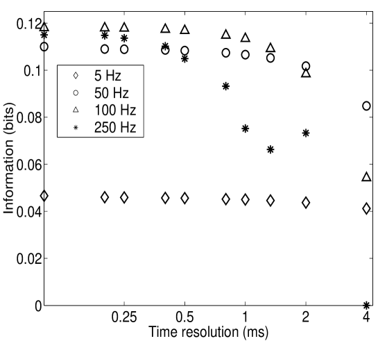
Figure 6: Panzeri, MS 2096

As an example, Figure 6 illustrates the impact of sampling precision on the full temporal information contained in 32 ms from a single model cell responding to two stimuli according to a Poisson process. The first stimulus elicits a constant response firing rate, the second stimulus elicits a response firing rate oscillating sinusoidally in time, exactly as in Figure 3. In Figure 6, the oscillation frequencies for the responses to the second stimulus were varied in the range 5-250 Hz. The result is that the timing precision has no effect on the information only if it is much smaller than the typical time scale of response parameter variations $\tau_{c}$. If $\Delta t\simeq\tau_{c}$, then information is strongly underestimated with respect to the infinite resolution limit.

The issue of the efficiency of information transmission for different timing precisions (i.e. how much of the total entropy is actually exploited for information transmission) is addressed in ?.

8 Synergy and redundancy in temporal information

How is information combined from a group of coding elements? Is the amount of information obtained from the whole pool of elements greater than the sum of that from each individual element (synergistic) or less than the sum (redundant)? Between these two cases, there can exist a situation where the information from each element is independent, and the total information thus increases linearly as the number of elements is increased. Two notions of “synergy” are of immediate relevance. The first is synergy/redundancy between assemblies of cells; the second is synergy between spikes (whether they are from the same cell or another).

Synergy between cells. We define the amount of synergy between cells as the total information from the ensemble of spike trains minus the sum of that from the individual cells (?, p. 268). The redundancy is simply the negative of this quantity. This means that, to second order, the synergy is simply the sum of the off-diagonal ($a\neq b$) elements of equation 15. This is because the first order terms (equation 14) of the information and the $a=b$ terms in the summation are identical for both the ensemble information and the sum of the individual cell informations, thus eliminating in the subtraction.

The amount of synergy between cells depends critically upon correlation. For synergistic coding, non-zero cross-correlation is needed. This can be seen from equation 15: in the absence of correlation $\gamma$ only the first term of $I_{tt}$ would survive, and we have shown this term to be less than or equal to zero, meaning that synergy cannot occur.

It is quite obvious that synergy may occur when the degree of correlation between cells is modulated by the stimulus. However, even when noise correlation is not stimulus dependent, it is possible to achieve synergistic coding. This is done by using the second, stimulus-independent, correlational component of $I_{tt}$ to increase the total information. This happens, for each pair of cells, when the noise correlation $\gamma_{ab}(t^{a}_{i},t^{b}_{j};s)$ is opposite in sign to the signal correlation $\nu_{ab}(t^{a}_{i},t^{b}_{j})$ for times $t^{a}_{i},t^{b}_{j}$. This basic mechanism of synergy for the temporal information is identical in principle to that considered for spikes counts in (?; ?; ?); it extends naturally to noise and signal correlations between time pairs $t^{a}_{i}$ and $t^{b}_{j}$.

Correlations between cortical neurons often oscillate and vary rapidly in sign with time (?). Our analysis shows that in this case, to obtain a maximally synergistic effect, the signal correlation should oscillate in counterphase with respect to the cross-correlogram and with similar frequency. This produces opposite signs of signal and noise correlation. If the signal was of lower frequency, the effect of cross-correlation would be washed away by its rapid change of sign with respect to the signal. The effect of the relative frequencies and phase of signal and noise variations with time is illustrated in Figure 7. We simulated two Poisson cells, responding to two stimuli as in Figure 3a, but with firing rate in response to the second stimulus being modulated at $f_{1}=10$ and $f_{2}=20$ Hz respectively. The signal correlation between the cells is in this simple case

$$\nu(t^{a},t^{b})\propto\sin(2\pi f_{1}t^{a})\sin(2\pi f_{2}t^{b}).$$ (22)

To generate a cross-correlation model that could be tuned to match the signal correlation frequency, the cross-correlation was chosen for both stimuli to be of the form

$$\gamma_{ab}(t^{a},t^{b};s)=\gamma exp(-|t^{a}-t^{b}|/\lambda)\sin(2\pi kf_{1}t^{a})\sin(2\pi kf_{2}t^{b}).$$ (23)

The cross-correlation function decayed exponentially, with time constant 25 ms, as a function of the time between spikes (?). The constant $\gamma$ in front of the correlation function was set either to 0 (no cross-correlation), to -1 (signal and noise in counter-phase), or to 1 (signal in phase with the noise). $k$ determined the relative timescales of signal and noise correlation oscillation, and was set to 1 for Figure 7 part A and 10 for part B. The information from the pair of cells observed simultaneously is compared with the summed single cell information in the Figure.

When the noise correlation between the cells is chosen to oscillate with the same frequency as the signal correlation does, synergy is obtained when signal and noise correlation are in counter-phase. Conversely high redundancy is obtained when they are in phase. When instead, signal and noise oscillate on very different time scales, correlations play a much less significant role. When response profiles of different neurons are independent, and little signal correlation is present, weakly stimulus modulated correlations do not affect information transmission at all (?; ?). This is important as signal correlation between cortical neurons was reported to be very small for stimulus sets of increasing complexity (?; ?; ?), and therefore correlations might be less important under natural conditions than when using artificial and limited laboratory stimuli.

The neuronal model used in this simulation is certainly far from realistic; however, the result discussed here is valid beyond the simple models used for the Figures. We note that when cross-correlations are stimulus dependent, then the third term of equation 15 also becomes non-zero, and additional interactions between response parameters can arise. They can be studied by specifying the stimulus dependence of correlations and taking into account also this information component.

In conclusion, this section shows that the contribution of cross-correlations to the representation of the external world can be more complex than what might be expected from naive visual inspection of cross-correlograms. This reinforces the need for a rigorous information theoretic analysis of the role of trial-by-trial correlations in solving complex encoding problems, like feature binding (?).

Synergy between spikes

Another notion of synergy, defined for single cells (as well as populations) and for the full temporal information, is synergy between spikes. Motivated by the notion that particular sequences of spikes may have a special role in encoding stimuli, ? recently introduced a synergy measure of this type. In that work, “events” (e.g. single spikes, or pairs of spikes occurring with a given time delay irrespective of whether there are other spikes in-between) are singled out from the whole spike train; the information carried by occurrence of single events was computed. ? considered the synergy to be the information from a complex event (e.g. a pair of spikes occurring at specified times) minus the information from each of those individual spikes constituting that pair.

Another way to measure the synergy between spikes that is suggested by the present analysis is to take into account their contribution to the information conveyed by the whole spike train. The contribution of single spikes to the whole spike train information is given by equation 14, and correspondingly the contribution of pairs of spikes is given by the sum of equations 14 and 15. Therefore the extent of synergy between pairs of spikes is simply the quantity given in equation 15 alone. The concept generalises to higher order interactions; ‘spike’ synergy is something which falls naturally out of the series expansion approach.

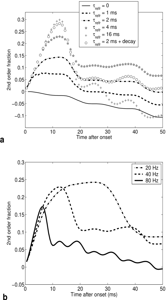
Figure 8: Panzeri, MS 2096

It is interesting to note that the introduction of a refractory period has an accompanying effect on the synergy between spikes, as measured by the fractional second order contribution to the overall temporal information. Figure 8a shows the effect of the refractory period on the synergy between spikes. This is shown for the example of a cell whose firing rate is modulated by a 40 Hz sinusoid for one stimulus as in the earlier Figures. The Figure compares a Poisson process with processes augmented with an absolute refractory period of between 1 and 16 ms, and also with another process which has a 2ms absolute refractory period, and an exponentially decaying autocorrelation with time constant 20 ms, reflecting a relative refractory period. It is apparent that for the Poisson process (in which spikes are not entirely independent because of the rate modulation) the second order contribution is small or negative. For longer refractory periods there is an increasing peak in the early period of the response. This effect appears to involve an interaction between the absolute refractory period and the time-constant of stimulus modulation of the rates; the stimulus modulation timescale determines the width of the spike-synergy peak (see Figure 8b), whereas the refractory period length determines its height.

It has been noted previously that the temporal correlations introduced into the spike train by refractoriness can have a beneficial effect on coding. This occurs by regularization of the higher firing rate parts of the response, producing a more deterministic relation between stimulus and response (?; ?). The present analysis confirms this effect, and adds several new facts: that the effect is second order in time, and that it involves interaction between the refractory and dominant stimulus-induced modulation timescales, such that the width of the period of increased information is determined by the stimulus frequency characteristics, whereas the amount of extra information is determined by the effective duration of refraction.

9 Analysis of neurophysiological data

In order to illustrate the specific advantages and the type of neurophysiological results that can be obtained with our series expansion method, we present here an example analysis of two cells recorded from the barrel cortex of adult normal anaesthetised Wistar rats. The two neurons presented were located in the D2 and C2 barrel column respectively. Each of the stimulation consisted of a 100 ms lasting upward deflection of one of the whiskers. For each neuron, the stimulus set was composed of its principal whisker and its eight surrounding whiskers, so that each of the whiskers that were likely to activate the cells were included in the stimulus set. 50 to 56 trials per whisker were available. The time onset of stimulation, as well as spike times, were recorded with 0.1 ms precision. (See ? for a complete description of the experimental methods). The information about which of the nine whiskers was stimulated was computed, both with the series expansion approach and using brute force estimation from response frequencies. Information from spike counts and spike times were both computed. For the latter, a resolution $\Delta t$ = 10 ms was used. Corrections for the upward bias originating from limited sampling were applied (see Appendix B). The range over which unbiased information measures could be obtained is discussed below and in Appendix B. Note that the probability scaling assumption was shown to be satisfied by both neurons in Figure 2.

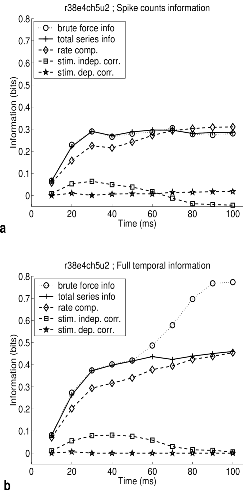
Figure 9: Panzeri, MS 2096

Figure 9a shows the spike count information analysis for the first neuron. Since the overall mean rate of the neuron across the 100 ms stimulation is 10 Hz, the series expansion is expected to be very good. Indeed, a comparison of the brute force and series spike count information shows that the two are essentially identical for the whole stimulation time range. As the two quantities are (after finite sampling corrections) unbiased in this time range, this is a very compelling verification of the validity of the series expansion method. In Figure 9b we report the spike times information analysis for the first neuron. It is evident that the brute force estimation of the full temporal information diverges rapidly after the first four to five time bins (i.e. after to 40-50 ms). This is due to failure of corrections for finite sampling, as expected by the rule of thumb for sampling corrections (see Appendix B). The spike times series expansion is a close match to the brute force estimator up to 40-50 ms, and no appreciable divergence due to finite sampling is visible, again as expected. This illustrates the clear superiority, in terms of sampling requirements, of the series expansion with respect to brute force evaluations. The separation of information into components, obtained using the series expansion, shows that most of the information is carried by the rate component. However, for this cell spike correlations contribute up to approximately 15% of the information in the spike times case. Note that this information in spike correlations is all contributed by the stimulus-independent component. This means that this little correlational information does not arise from modulation of the autocorrelogram with stimulus, but from the interplay of signal and noise correlations. The peak across time for the spike count information was 0.31 bits; the full temporal information obtained with 10 ms resolution was of 0.41 bits at time T = 50 ms. This shows that a neuron can transmit appreciable temporal information within a fraction of one mean interspike interval. This possibility was predicted by our mathematical analysis of coding regimes. Finally, it is interesting to note that this neuron in the first 10 ms of response carried on average more than 3 bits per each spike emitted.

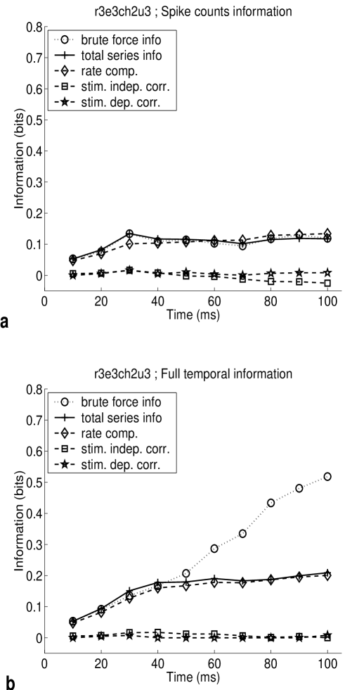
Figure 10: Panzeri, MS 2096

Figure 10 reports the information time course for the second neuron. Its mean rate across 100 ms was 16 Hz. Also in this second case the information for the spike counts obtained with the series expansion coincided with that obtained by the brute force method, thus confirming the reliability of the series expansion. When considering spike times, series expansion and brute force evaluation are very close up to 40-50 ms. After 50 ms, the brute force evaluation cannot be corrected effectively for finite sampling, and thus it starts to diverge. The peak spike count information was 0.13 bits; the peak spike timing information was 0.20 bits. As before, significant temporal information is transmitted within one typical interspike interval. The component analysis indicates that, unlike the first cell, this second cell transmits information by mean firing rate modulations only, and correlations between spikes do not transmit any information.

The above two cells were shown only for illustrative purposes, rather than to make any general point about the information properties of barrel cortex neurons. This illustration shows that i) the series expansion method can give reliable and testable results, ii) when used to compute information in spike times, it has considerable advantages in terms of data size requirements; and iii) it can effectively quantify the contributions of different encoding mechanisms to neuronal information transmission.

10 Discussion

We have demonstrated that the (?) information contained in the specification of the times of spike emission of a population of cells can be broken up into a series of terms each quantifying the contribution of a different encoding mechanism, just as the information contained in the spike counts from a population can (?). Although it can be applied only to a limited range of time windows, the use of this series approach has a number of advantages over brute force computation for both the understanding of the theory of coding with spike trains, and for the analysis of neurophysiological data.

A first advantage of this approach is that it necessarily compares the contributions of different information-bearing parameters on correct and equal terms, and shows how they combine to yield the full information available from the spike train. A second advantage of the series expansion method is that it requires much less data sampling than a brute force approach, in order to obtain unbiased and reliable information measures. This is because the information is computed by using only the subset of the possible variables characterising the spike train which carry the most information in the short time limit. Therefore the complexity of the response space is reduced in the way that preserves the most information. A third interesting feature of the method present here is that it does not assume that the neuronal response space is a vector space, as e.g. Principal Component Analysis (?) does. Since sensory systems are non-linear, this is a property that has to be satisfied by any method for studying neuronal information encoding (?; ?). Fourth, the series expansion approach is a method to quantify the full temporal information that can be extracted from the spike train by an ideal observer, and does not depend on the validity of a stimulus-response model, and is not specific to a particular stimulus decoder. Therefore it provides information values against which the performance of encoding/decoding models can be assessed (?; ?).

The observation timescales with which spike trains are studied depend upon the questions which are being asked. Many authors, particularly those with a perspective from the field of psychophysics, have examined windows of data up to several seconds long. The justification is that, in certain tasks (?), psychophysical performance increases up to these timescales, as does the ability to discriminate stimuli based upon counting the spikes of a single cell (as counting for longer allows noise to be averaged out). The techniques discussed in the current paper are inapplicable to such long time windows (although other techniques such as direct calculation of the spike count information for a single cell do apply). The authors would like to comment that the study of neural coding is often considered as a precursor to, or partner of, the study of computation or information processing in the nervous system. To understand the computational architecture of the brain, it is necessary to understand the nature of the symbols which are processed. Accepting that single neurons are the primary information processing units of the brain, these symbols must exist on timescales which are “seen” by single cells, which may be as low as a membrane time-constant, or longer if additional integrative processes are enacted. It is neural coding on single cell timescales which determines computation, and which motivates the current work. Since perceptual processes are unlikely to be uniform in time, such a strategy might also elucidate some of the computations underlying perception at longer timescales.

The work presented here is not only relevant as a tool for neurophysiological data analysis. It allows also analytical studies of the statistical properties of population spike trains, such as refractoriness, autocorrelation, and timing relationships between cells, to be conducted with regard to understanding which parts of the full temporal information they contribute to and which they do not. Here we have used this formalism to relate precisely the time scale of response parameter variations to transitions between spike count and temporal encoding regimes; to show that the impact on information representations of stimulus-independent trial-by-trial correlations depends crucially on their interplay with the signal correlation; and to show that the neuronal refractory period can lead to synergy between spikes. A further understanding of how other parameters of biophysical relevance can be adjusted to maximise encoding capacity can be reached by the use of the formalism presented here.

One most interesting finding often reported in experimental studies of neuronal information transmission is that sensory neurons transmit most of the information within one mean interspike interval, and single spikes carry a lot of information (?). Thus high spike timing precision and rate coding may coexist in sensory neuron, as the rate code has to be evaluated in a short window. This has led some authors to conclude that under these conditions the distinction between rate and temporal encoding may become blurred (see ?, p. 119). However, differences between temporal and rate encoding and rate coding can be defined and be present even under conditions of such rapid processing (?; ?). Our study advances the understanding of the distinction between temporal and rate encoding when the relevant window for information transmission is short. In fact, our work explicitly relates response variations time scales to transitions between coding regimes, and shows that under some conditions a substantial amount of information can be encoded purely temporally within a fraction of one interspike interval (see section 6). Indeed, the example analysis of two neurons in the rat barrel cortex shows that this is not only a theoretical possibility, but that it can be realised by sensory neurons.

? argue that because the interspike interval in the responses of cortical neurons is highly variable, the rapid information transmission achieved by the cerebral cortex (i.e. substantial information being transmitted in one ISI or less) must imply redundancy of signal. Their argument is based on the idea that to obtain reliability in short timescales it is necessary to average away the large observed variability of individual ISIs by replicating the signal through many similar neurons. In other words, the need for rapid information transmission should strongly constrain the cortical architecture. Our study demonstrates precisely the opposite. The fact that the first order temporal information transmitted by a population is simply the sum of all single-cell contributions (equation 14) demonstrates that it is not necessary to transmit many copies of the same signal to ensure rapid and reliable transmission. If each cell contributes some non-identical information about the stimuli, this will sum up in less than one ISI, and high population information rates can be achieved.

We finally note that an earlier work by DeWeese (?; ?) has previously reported an elegant analytical study of the impact of interaction between spikes of information transmission in single cells. This study made use of a cluster-expansion formalism derived from statistical mechanics. The results obtained by DeWeese in this way are close to what we obtained in the single cell case. The only difference is that in DeWeese’s equations the summation over time in the quadratic term of second derivative of the information is restricted to pairs of time bins different from each other. However, this work reports several advances with respect to the earlier work of DeWeese. In fact, we computed the information carried by an ensemble of cells, instead of by single cells only. We separated the information into different components, each reflecting different encoding mechanisms. We also studied the transition between spike count and temporal encoding regimes. The power series formalism makes the conditions under which the series converges transparent; this issue is much less clear with a cluster expansion (see e.g. (?) p. 41). Unlike in (?), corrections for finite sampling were introduced here. This last development is essential when using the method for studying information transmission in real neurons.

In conclusion, a full understanding of the coding properties of a neural system cannot be achieved simply by computing the total information about the stimuli contained in its spike trains; rather, it is necessary to at the very least discover how this total is comprised from the individual information-bearing parameters. The results that we have presented here encourage us to think that this is possible.

Appendix A

In this Appendix we show that, under the assumptions summarized in section 5, the only responses contributing to the transmitted information up to order $k$ are the spike patterns with up to $k$ spikes in total. Thus the power expansion in the short time window length $T$ is related to the expansion in the total number of spikes emitted by the population. We also compute the only non-zero response probabilities up to second order, which are the only ones contributing to the first two information derivatives. We give the proof for finite temporal precision.

Consider the response to stimulus $s$. The probability of observing one spike in the bin centered at $t^{a}_{i}$, averaged over all possible patterns of spikes occurring in other bins, is $r_{a}(t^{a}_{i};s)\Delta t$. Now, note that the assumption specified by equation 6 implies that the probability of a single spike, the observation of any pattern of other spikes, also scales proportionally to $\Delta t$:

$$P(t^{a}_{i}|t^{b}_{j}\cdots t^{f}_{k};s)\propto\Delta t$$ (A.1)

Thirdly, we use the well known theorem on compound probabilities to write down the following chain rule for the probability of observing a pattern $t^{a}_{i}t^{b}_{j}\cdots t^{f}_{k}$ of $k$ spikes when stimulus $s$ is presented:

$$P(t^{a}_{i}t^{b}_{j}\cdots t^{f}_{k};s) = P(t^{a}_{i}|t^{b}_{j}\cdots t^{f}_{k};s)P(t^{b}_{j}|\cdots t^{f}_{k};s)\cdots P(t^{f}_{k};s)$$ (A.2)

This means that a probability of $k$ spikes is a product of $k$ conditional probabilities of emission of each of the spikes given the presence of other spikes in the pattern. Since, as proven above, each of the $k$ terms of this product is proportional to $\Delta t$, probabilities of $k$-plets of spikes scale as $(\Delta t)^{k}$. From this scaling property, from the definition of information, equation 1, and from the logarithm series expansion, equation 13, it follows that, for the computation of the first $k$ information derivatives, only response probabilities with up to $k$ spikes are needed, and they can be truncated at the $k$-th order in $\Delta t$. Responses with more than $k$ spikes do not contribute to the first $k$ information derivatives.

Finally we compute the response probabilities of up to two spikes, truncated at the second order in $\Delta t$. The probability of observing just two spikes at $t_{1}^{a},t_{2}^{b}$ is, up to $O(\Delta t^{2})$, given by the product of $P(t_{1}^{a}|t_{2}^{b};s)$ (from equation 6) and $r_{b}(t_{2}^{b};s)\Delta t$ (the latter factor quantifying at first order the probability of one spike in $t_{2}^{b}$):

$$P(t_{1}^{a}t_{2}^{b};s) = {1\over 2}\overline{r}_{a}(t_{1}^{a};s)\overline{r}_{b}(t_{2}^{b};s)\left[1+\gamma_{ab}(t_{1}^{a},t_{2}^{b};s)\right](\Delta t)^{2}+O(\Delta t^{3})$$ (A.3)

The probability of two spikes is divided by two to prevent over-counting due to equivalent permutations, rather than restrict the sum over events to non-equivalent permutations, as was done in ?. The probability $P(t_{1}^{a};s)$ of observing just one spike at $t_{1}^{a}$ is given, up to order $\Delta t^{2}$, by the product of $r_{b}(t_{2}^{b};s)\Delta t$ and the probability of not observing any other spike than that at $t_{1}^{a}$:

$$P(t_{1}^{a};s) = r_{a}(t_{1}^{a};s)\Delta tP({\rm~{}no~{}spikes~{}but}~{}t_{1}^{a};s)+O(\Delta t^{3})$$ (A.4)

$$= r_{a}(t_{1}^{a};s)\Delta t\left(1-\sum_{b=1}^{C}\sum_{t_{2}^{b}}P(t_{2}^{b}|t_{1}^{a};s)-\sum_{b,c}\sum_{t_{2}^{b}t_{3}^{c}}P(t_{2}^{b}t_{3}^{c}|t_{1}^{a})-\cdots\right)$$

$$= r_{a}(t_{1}^{a};s)\Delta t\left(1-\Delta t\sum_{b=1}^{C}\sum_{t_{2}^{b}}\overline{r}_{b}(t_{2}^{b};s)\left[1+\gamma_{ab}(t_{1}^{a},t_{2}^{b};s)\right]\right)$$

$$+ O(\Delta t^{3})$$

The probability of no cells at all firing, up to $\Delta t^{2}$, can be obtained by subtracting from 1 all the response probabilities which are non-zero at second order.

The probability expansion in the infinite temporal precision limit can be obtained along the same lines, by replacing probabilities with probability densities, and using equation 11.

Appendix B

When considering neurophysiological data, the information quantities have to be evaluated from response probabilities obtained from a limited number of trials per stimulus, $N_{s}$. This induces an upward systematic error, or bias, in the information measures. The systematic error has to be evaluated and subtracted in order to obtain unbiased information measures. In this appendix we briefly report how the bias is computed and corrected for in the different information estimation methods.

The bias correction is a simple formula, which is slightly different when considering the information is calculated directly from the Shannon formula (equations 1 and 2) by “brute force” estimation of response frequencies, or when considering the information computed by the series expansion (see ?,?):

$$\delta I_{\rm bruteforce}=\frac{\sum_{s\in\cal S}(R_{s}-1)-(R-1)}{2N\ln 2};\qquad\delta I_{\rm series}=\frac{\sum_{s\in\cal S}(R_{s})-R}{2N\ln 2}$$ (B.1)

where $N$ is the total number of trials (across all stimuli), and $R$ is the number of relevant response classes across all stimuli (i.e. the number of different responses with non-zero probability of being observed). $R_{s}$ is the number of relevant response classes to stimulus s (?). It is intuitive that the number of trials per stimulus $N_{s}$ should be big when compared to the number of response classes $R$ in order to get good enough sampling of conditional responses, and therefore reliable bias correction. When a Bayes procedure (that takes into account that some response classes may not be observed just because of local undersampling) is used to estimate the number of relevant bins, reliable bias corrections can be obtained when $N_{s}$ is equal or higher than the number of response classes $R$. This gives a useful rule of thumb for evaluating the range in which the bias corrections still work.

For the brute force full temporal information (equation 1), the response space is that of all the possible temporal spike patterns, and the number of possible responses is $2^{Cd}$, $d=T/\Delta t$ being the number of time bins in which the window is digitised. The situation is very different when the information is computed by the series expansion approach. For the first order spike times information, $R$ is the number of non-zero bins of the dynamic rate function, which is at most $Cd$. For the second order spike times information, $R$ is the number of relevant bins in the space of pairs of spike firing times, which is at most $Cd(d-1)/2\;+C(C-1)d(d+1)/4$. Therefore the number of trials needed to effectively correct for the bias grows only linearly when $C$ or $d$ is increased if the first order term is considered, and only quadratically when also the second order term is included. Considering that the growth of the data size required for the brute force evaluation from the Shannon formula is exponential, there is a clear advantage in terms of data size when using the series approach developed here. Some simulation examples of effectiveness of bias removal procedures for the series expansion method were reported in ?.

As an example, when 50-55 trials per stimulus are available for information analysis of single cells (as in the example reported here), the brute force computation is unbiased only up to 4-5 time bins, and the series expansion is unbiased up to 9-10 time bins. The spike count information quantities of course require much less data than the corresponding spike times quantities. They are thus well corrected for bias for the whole range in which the full temporal information measures are reliable.

Figure Captions

Figure 1: The accuracy of the first and second order approximations to the full information in the spike times of a single cell with Poisson responses to two stimuli. The cell responded to stimulus 1 with a constant (in time) rate of 30 spikes/sec., and to stimulus 2 with a spike rate oscillating sinusoidally around 30 spikes/sec. with period 2 ms and amplitude 30 spikes/sec.

Figure 2: The scaling relationship between the average conditional firing rate (computed as the average probability of observing a spike at one time, given that a spike has been observed at another time, divided by the bin width $\Delta t$) and the bin width of observation. The relationship is shown for two cells from the rat barrel cortex.

Figure 3: Comparison of the full temporal and spike count information. (A) The modulation of the firing rates of a single non-homogeneous Poisson neuron by two stimuli. (B) The evolution of the full temporal and the spike count information as the time window is increased in width from the first instance of stimulus related responses

Figure 4: The effect of the frequency of stimulus modulation of the rates. a Full temporal information. b Purely temporal information only. The main requirement for temporal contribution to the information can be seen easily in the comparison of these two figures – fast fluctuation of the firing rates in comparison to the timescale of observation.

Figure 5: A situation in which stimulus dependent correlation in spike timing between cells can make a sizeable (but nevertheless second order) contribution to the total information, via component 2c of the temporal information. (a) Correlation function. (b) Resulting components of the full temporal information. Component 2c dominates. Note that the corresponding spike count component was more than ten times smaller over the whole time range.

Figure 6: The effect of precision of spike timing on the information available from 32 ms of the response of a single simulated neuron. We used an absolute refractory period of 4 ms in this simulation (in order to have at most one spike per time bin for all the precisions ‘used). The data obtained with the continuous-time limit (obtained by numerical integration) are included as the y-intercept information values.

Figure 7: The effect of the relative frequencies and phase of signal and noise temporal variations in achieving synergistic coding. (A) With signal and noise correlation oscillating with identical timescales. The line marked with the star symbol indicates synergistic coding in this case, as it falls above the sum of single cells’ information. (B) Noise correlation oscillating ten times faster than signal correlation.

Figure 8: Synergy between spikes, measured by the fraction of the temporal information contained in the second order terms. (A) Comparison of a Poisson process with processes augmented with absolute refractory periods. In one case a relative refractory period with exponential autocorrelation is also added (circles). (B) The interaction of a 4 ms refractory period with stimulus-induced modulation frequency, for three different modulation frequencies.

Figure 9: (a): The time course of the information in the spike counts for a neuron located in the D2 barrel column of the rat cerebral cortex. The information obtained with the brute force method (equation 2, indicated with $\circ$) is compared to that obtained with the series expansion at second order ($+$). The three components of the series expansion information are also presented (rate ($\diamond$); stimulus independent correlational (box); stimulus dependent correlational ($\star$)). (b): The time course of information carried by spike times of the same neuron, computed with a 10 ms precision. Notation as in (a). The ‘rate’ component in this case of course refers to the dynamic firing rate across the time window, rather than anything to do with a spike count code.

Figure 10: The spike count and spike times information time course for a second neuron located in the C2 barrel column. Notations as in Figure 9.

References

- [1]
- [2] [] Abbott, L. F. and Dayan, P. (1999). The effect of correlated variability on the accuracy of a population code, Neural Comp. 11: 91–101.
- [3]
- [4] [] Adrian, E. D. (1926). The impulses produced by sensory nerve endings: Part I, J. Physiol. (Lond.) 61: 49–72.
- [5]
- [6] [] Bair, W. and Koch, C. (1996). Temporal precision of spike trains in extrastriate cortex of the behaving macaque monkey, Neural Computation 8(6): 779–786.
- [7]
- [8] [] Berry II, M. J. and Meister, M. (1998). Refractoriness and neural precision, J. Neurosci. 18(6): 2200–221.
- [9]
- [10] [] Bialek, W., Rieke, F., de Ruyter van Steveninck, R. R. and Warland, D. (1991). Reading a neural code, Science 252: 1854–1857.
- [11]
- [12] [] Borst, A. and Theunissen, F. E. (1999). Information theory and neural coding, Nature Neuroscience 2: 947–957.
- [13]
- [14] [] Brenner, N., Strong, S. P., Koberle, R., Bialek, W. and de Ruyter van Steveninck, R. (1999). Synergy in a neural code, Neural Computation p. In press.
- [15]
- [16] [] Britten, K., Shadlen, M. N., Newsome, W. T. and Movshon, J. A. (1992). The analysis of visual-motion - a comparison of neuronal and psychophysical performance, J. Neurosci. 12: 4745–4765.
- [17]
- [18] [] Buracas, G. T., Zador, A. M., de Weese, M. R. and Albright, T. D. (1998). Efficient discrimination of temporal patterns by motion-sensitive neurons in primate visual cortex, Neuron 20: 959–969.
- [19]
- [20] [] Corthout, E., Uttl, B., Walsh, V., Hallett, M. and Cowey, A. (1999). Timing of activity in early visual cortex as revealed by transcranial magnetic stimulation, Neuroreport 10: 2631–2634.
- [21]
- [22] [] Cover, T. M. and Thomas, J. A. (1991). Elements of information theory, John Wiley, New York.
- [23]
- [24] [] de Ruyter van Steveninck, R. R., Lewen, G. D., Strong, S. P., Koberle, R. and Bialek, W. (1997). Reproducibility and variability in neural spike trains, Science 275: 1805–1808.
- [25]
- [26] [] DeAngelis, G. C., Ghose, G. M., Ohzawa, I. and Freeman, R. D. (1999). Functional micro-organization of primary visual cortex; receptive field analysis of nearby neurons, J. Neurosci. 19: 4046–4064.
- [27]
- [28] [] deCharms, R. C. and Merzenich, M. M. (1996). Primary cortical representation of sounds by the coordination of action potentials, Nature 381: 610–613.
- [29]
- [30] [] DeWeese, M. (1995). Optimization principles for the neural code, PhD thesis, Princeton University.
- [31]
- [32] [] DeWeese, M. (1996). Optimization principles for the neural code, Network 7: 325–331.
- [33]
- [34] [] Gawne, T. J., Kjaer, T. W., Hertz, J. A. and Richmond, B. J. (1996). Adjacent visual cortical complex cells share about 20% of their stimulus-related information, Cerebral Cortex 6: 482–489.
- [35]
- [36] [] Heller, J., Hertz, J. A., Kjaer, T. W. and Richmond, B. J. (1995). Information flow and temporal coding in primate pattern vision, J. Comp. Neurosci. 2: 175–193.
- [37]
- [38] [] König, P., Engel, A. K. and Singer, W. (1995). Relation between oscillatory activity and long-range synchronization in cat visual cortex, Proc. Natl. Acad. Sci. USA 92: 290–294.
- [39]
- [40] [] Lebedev, M. A., Mirabella, G., Erchova, I. and Diamond, M. E. (2000). Experience-dependent plasticity of rat barrel cortex: redistribution of activity across barrel-columns, Cerebral Cortex 10: 23–31.
- [41]
- [42] [] MacKay, D. and McCulloch, W. S. (1952). The limiting information capacity of a neuronal link, Bull. Math. Biophys. 14: 127–135.
- [43]
- [44] [] Mechler, F., Victor, J. D., Purpura, K. P. and Shapley, R. (1998). Robust temporal coding of contrast by V1 neurons for transient but not steady-state stimuli, J. Neurosci. 18(16): 6583–6598.
- [45]
- [46] [] Optican, L. M. and Richmond, B. J. (1987). Temporal encoding of two-dimensional patterns by single units in primate inferior temporal cortex: III. Information theoretic analysis, J. Neurophysiol. 57: 162–178.
- [47]
- [48] [] Oram, M. W., Földiák, P., Perrett, D. I. and Sengpiel, F. (1998). The ’Ideal Homunculus’: decoding neural population signals, Trends in Neurosciences 21(6): 259–265.
- [49]
- [50] [] Panzeri, S., Biella, G., Rolls, E. T., Skaggs, W. E. and Treves, A. (1996a). Speed, noise, information and the graded nature of neuronal responses, Network 7: 365–370.
- [51]
- [52] [] Panzeri, S., Schultz, S. R., Treves, A. and Rolls, E. T. (1999). Correlations and the encoding of information in the nervous system, Proc. R. Soc. Lond. B 266: 1001–1012.
- [53]
- [54] [] Panzeri, S. and Treves, A. (1996). Analytical estimates of limited sampling biases in different information measures, Network 7: 87–107.
- [55]
- [56] [] Riehle, A., Grun, S., Diesmann, M. and Aertsen, A. M. H. J. (1997). Spike synchronization and rate modulation differentially involved in motor cortical function, Science 278: 1950–1953.
- [57]
- [58] [] Rieke, F., Warland, D., de Ruyter van Steveninck, R. R. and Bialek, W. (1996). Spikes: exploring the neural code, MIT Press, Cambridge, MA.
- [59]
- [60] [] Rolls, E. T., Tovee, M. and Panzeri, S. (1999). The neurophysiology of backward visual masking: Information analysis, J. Cognitive Neurosci. 11: 335–346.
- [61]
- [62] [] Rolls, E. T., Treves, A. and Tovée, M. J. (1997). The representational capacity of the distributed encoding of information provided by populations of neurons in primate temporal visual cortex, Exp. Brain Res. 114: 149–162.
- [63]
- [64] [] Schultz, S. R. and Panzeri, S. (2000). Temporal correlations and neuronal spike train entropy. Submitted to Physical Review Letters.
- [65]
- [66] [] Shadlen, M. N. and Newsome, W. T. (1998). The variable discharge of cortical neurons: implications for connectivity, computation and coding, J. Neurosci. 18(10): 3870–3896.
- [67]
- [68] [] Shannon, C. E. (1948). A mathematical theory of communication, AT&T Bell Labs. Tech. J. 27: 379–423.
- [69]
- [70] [] Singer, W., Engel, A. K., Kreiter, A. K., Munk, M. H. J., Neuenschwander, S. and Roelfsema, P. (1997). Neuronal assemblies: necessity, signature and detectability, Trends in Cognitive Sciences 1: 252–261.
- [71]
- [72] [] Skaggs, W. E., McNaughton, B. L., Gothard, K. and Markus, E. (1993). An information theoretic approach to deciphering the hippocampal code, in S. Hanson, J. Cowan and C. Giles (eds), Advances in Neural Information Processing Systems, Vol. 5, Morgan Kaufmann, San Mateo, pp. 1030–1037.
- [73]
- [74] [] Strong, S., Koberle, R., de Ruyter van Steveninck, R. and Bialek, W. (1998). Entropy and information in neural spike trains, Physical Review Letters 80: 197–200.
- [75]
- [76] [] Theunissen, F. E. and Miller, J. P. (1995). Temporal encoding in nervous systems: a rigorous definition, J. Comput. Neurosci. 2: 149–162.
- [77]
- [78] [] Thorpe, S., Fize, D. and Marlot, C. (1996). Speed of processing in the human visual system, Nature 381: 520–522.
- [79]
- [80] [] Tovée, M. J., Rolls, E. T., Treves, A. and Bellis, R. P. (1993). Information encoding and the response of single neurons in the primate temporal visual cortex, J. Neurophysiol. 70: 640–654.
- [81]
- [82] [] Vaadia, E., Haalman, I., Abeles, M., Bergman, H., Prut, Y., Slovin, H. and Aertsen, A. (1995). Dynamics of neuronal interactions in monkey cortex in relation to behavioural events, Nature 373: 515–518.
- [83]
- [84] [] Victor, J. D. and Purpura, K. P. (1996). Nature and precision of temporal coding in visual cortex: a metric space analysis, J. Neurophysiol. 76: 1310–1326.
- [85]
- [86] [] Victor, J. D. and Purpura, K. P. (1997). Metric space analysis of spike trains: theory, algorithms and applications, Network 8: 127–164.
- [87]
- [88] [] Victor, J. D. and Purpura, K. P. (1998). Spatial phase and the temporal structure of the response to gratings in V1, J. Neurophys. 80: 554–571.
- [89]