1S-2S Spectrum of a Hydrogen Bose-Einstein Condensate
published Physical Review A 61, 33611 (2000)

Abstract

We calculate the two-photon $1S$-$2S$ spectrum of an atomic hydrogen Bose-Einstein condensate in the regime where the cold collision frequency shift dominates the lineshape. WKB and static phase approximations are made to find the intensities for transitions from the condensate to motional eigenstates for $2S$ atoms. The excited state wave functions are found using a mean field potential which includes the effects of collisions with condensate atoms. Results agree well with experimental data. This formalism can be used to find condensate spectra for a wide range of excitation schemes.

I Introduction

In the recent experimental observation of Bose-Einstein condensation (BEC) in atomic hydrogen [2], the cold collision frequency shift in the $1S$-$2S$ photoexcitation spectrum [3] signalled the presence of a condensate. The shift arises because electronic energy levels are perturbed due to interactions, or collisions, with neighboring atoms. In the cold collision regime, the temperature is low enough that the $s$-wave scattering length, $a$, is much less than the thermal de Broglie wavelength, $\lambda_{T}=\sqrt{h^{2}/2\pi mk_{B}T}$, and only $s$-waves are involved in the collisions[4].

The cold collision frequency shift has also been studied in the hyperfine spectrum of hydrogen in cryogenic masers [5], and cesium [6, 7, 8] and rubidium [9] in atomic fountains. Theoretical explanations of these results and other work on the hydrogen $1S$-$2S$ spectrum [10, 11] have focused on the magnitude of the shift, as opposed to a lineshape. In this article we present a calculation of the hydrogen BEC $1S$-$2S$ spectrum. We also describe how the formalism can be used for other atomic systems and experimental conditions.

A The Experiment

The experiment is described in [2, 3], and we summarize the important aspects here. Hydrogen atoms in the $1S$, $F=1$, $m_{F}=1$ state are confined in a magnetic trap and evaporatively cooled. The hydrogen condensate is observed in the temperature range $30$-$70$ $\mu$K and the condensate fraction never exceeds a few percent. Nevertheless, the peak density in the normal cloud is almost two orders of magnitude lower than in the condensate and in this study we will neglect the presence of the noncondensed gas.

The two-photon transition to the metastable $2S$, $F=1$, $m_{F}=1$ state ($\tau=122$ ms) is driven by a 243 nm laser beam which passes through the sample and is retroreflected. In this configuration, an atom can absorb one photon from each direction. This results in Doppler-free excitation for which there is no momentum transferred to the atom and no Doppler-broadening of the resonance. An atom can also absorb two co-propagating photons and receive a momentum kick. This is Doppler-sensitive excitation, and the spectrum in this case is recoil shifted and Doppler-broadened. The photo-excitation rate is monitored by counting $122$ nm fluorescence photons from the excited state. For a typical laser pulse of $500$ $\mu$s, fewer than 1 in $10^{4}$ of the atoms are promoted to the $2S$ state. $2S$ atoms experience the same trapping potential as $1S$ atoms because the magnetic moment is the same for both states, neglecting small relativistic corrections.

The natural linewidth of the $1S$-$2S$ transition is $1.3$ Hz, but the experimental width, at low density and temperature, is limited by the laser coherence time. The narrowest observed spectra, obtained when studying a noncondensed gas, have widths of a few kHz [12]. For the condensate, the cold collision frequency shift is as much as one MHz and it dominates the lineshape.

B Mean Field Description of the Spectrum

The frequency shift in maser and fountain experiments has traditionally been described using the quantum Boltzmann equation[5, 6, 9]. In this picture, the frequency shift is the net result of the small collisional phase shifts arising from forward scattering events in the gas. A mean field description, however, is more convenient for studying an inhomogeneous Bose-Einstein condensate. We will derive this picture in detail, but we summarize the results here. Collisions add a mean field energy to the atom’s potential energy. For a $2S$ atom excited out of a condensate the mean field term is $\delta E_{2S}({\bf r})=4\pi\hbar^{2}a_{1S-2S}n_{1S}({\bf r})/m$. For a $1S$ condensate atom the mean field term is $\delta E_{1S}({\bf r})=4\pi\hbar^{2}a_{1S-1S}n_{1S}({\bf r})/m$. (The fraction of excited $2S$ atoms is small, so $2S$-$2S$ interactions can be neglected.) The ground state $s$-wave triplet scattering length has been calculated accurately ($a_{1S-1S}=0.0648$ nm[13]). The $1S$-$2S$ scattering length, however, is less well known ($a_{1S-2S}=-1.4\pm 0.3$ nm from experiment [3] and -2.3 nm from theory [14]).

We denote the sum of the magnetic trap potential, $V({\bf r})$, and the mean field energy, $\delta E_{x}({\bf r})$, as the effective potential, $V_{x}^{eff}({\bf r})$ (Fig. 1). Here $x$ is either $1S$ or $2S$. For $1S$ condensate atoms, the effective potential in the condensate is flat. Because $a_{1S-2S}<0$ and the condensate density is large, $2S$ atoms experience a stiff attractive potential in the condensate which supports many bound $2S$ motional states.

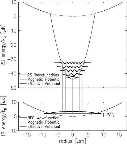
FIG. 1.: Effective potentials for $1S$ atoms in the condensate and excited $2S$ atoms. Selected single particle wave functions are displayed at the height corresponding to their energy. The dashed lines are the magnetic trapping potential $V({\bf r})$, which is identical for $1S$ and $2S$ atoms. The thin solid lines are the effective potentials, which include the mean field interaction energy. The vertical light solid lines indicate allowed Doppler-free transitions from the condensate, which must preserve mirror symmetry. The potentials and condensate wave function are for a peak condensate density of $5\times 10^{15}$ cm^-3 and a magnetic trap oscillation frequency of 4 kHz, which are characteristic conditions for a hydrogen BEC and a strong confinement axis of the trap [1,2]. The scattering lengths used in the calculations are $a_{1S-1S}=0.0648$ nm and $a_{1S-2S}=-1.4$ nm, and the chemical potential is $\mu/k_{B}\approx 2~{}\mu$K. The $2S$ levels form a near continuum of motional states in an anisotropic three dimensional trap.

The $1S$-$2S$ spectrum consists of transitions from the condensate to $2S$ motional eigenstates of the effective $2S$ potential. For Doppler-free excitation, the final states are bound in the BEC well. Doppler-sensitive excitation populates states which lie about $\hbar^{2}k_{0}^{2}/2mk_{B}=643$ $\mu$K above the bottom of the $2S$ potential, where $\hbar k_{0}$ is the momentum carried by two laser photons. The latter states extend over a region much greater than the condensate. Because the excited levels are so different for Doppler-free and Doppler-sensitive excitation, we must treat the two spectra independently.

The rest of this article presents a derivation of the effective potentials and a quantum mechanical calculation of the BEC $1S$-$2S$ spectrum.

II 1S-2S Photoexcitation Spectrum of a Hydrogen Bose-Einstein Condensate

A Hamiltonian

We start with the many-body Hamiltonian for a system with $N$ atoms,

$$H=\sum_{j=1}^{N}\left({{p}_{j}^{2}\over 2m}+H^{int}_{j}+V({\bf{r}}_{j})\right)+H^{las}+H^{coll},$$ (1)

where ${\bf{p}}_{j}$, ${\bf{r}}_{j}$, and $H^{int}_{j}$ are the momentum operator, position operator, and internal state Hamiltonian respectively for particle $j$. $V({\bf r})$ is the magnetic trapping potential, which is the same for $1S$ and $2S$ atoms.

$H^{las}$ is the atom-laser interaction. After making the rotating wave approximation, it can be written

$$H^{las}=\sum_{j=1}^{N}{\hbar\Omega({\bf{r}}_{j})\over 2}\left[(|2S\rangle\langle 1S|)_{j}e^{-i4\pi\nu t}+(|1S\rangle\langle 2S|)_{j}e^{i4\pi\nu t}\right],$$ (2)

where $\nu$ is the frequency of the laser field ($2h\nu\approx E_{2S}-E_{1S}\equiv E_{1S-2S}$ on resonance). The laser beam is uniform over the condensate, so we treat the excitation as a standing wave consisting of two counter-propagating plane waves. The effective 2-photon Rabi frequency for Doppler-free excitation [15],

$$\Omega_{DF}({\bf{r}})=\Omega_{DF}={2M_{2S,1S}\over 3\pi^{2}\hbar c}\left({\alpha\over 2R_{\infty}}\right)^{3}I,$$ (3)

is uniform in space. Here, $I$ is the laser intensity in each direction, $M_{2S,1S}=11.78$ [16] is a unitless constant, $c$ is the speed of light in vacuum, $\alpha$ is the fine structure constant, and $R_{\infty}$ is the Rydberg constant. For Doppler-sensitive excitation,

$$\Omega_{DS}({\bf{r}})=\Omega_{DS}({\rm e}^{ik_{0}z}+{\rm e}^{-ik_{0}z}),$$ (4)

where $\Omega_{DS}=\Omega_{DF}/2$.

$H^{coll}$ describes the effects of two-body elastic collisions. In the cold collision regime, the interaction can be represented by a shape independent pseudopotential[17] corresponding to a phase shift per collision of $ka$, where $\hbar{k}$ is the momentum of each of the colliding particles in the center of mass frame,

$$H^{coll} = {4\pi\hbar^{2}\over m}\sum_{i<j}^{N}\delta({\bf{r}}_{i}-{\bf{r}}_{j})\left[a_{1S-1S}(|1S\rangle\langle 1S|)_{i}(|1S\rangle\langle 1S|)_{j}+a_{1S-2S}(|e^{3}\Sigma^{+}_{u}\rangle\langle e^{3}\Sigma^{+}_{u}|)_{ij}\right.$$ (6)

$$\left.+a_{2S-2S}(|2S\rangle\langle 2S|)_{i}(|2S\rangle\langle 2S|)_{j}\right].$$

The sum is over $N(N-1)/2$ distinct pairwise interaction terms. The $1S$-$2S$ interaction projection operator is written in terms of

$$|e^{3}\Sigma^{+}_{u}\rangle_{ij} = {|1S\rangle_{i}|2S\rangle_{j}+|2S\rangle_{i}|1S\rangle_{j}\over\sqrt{2}}$$ (7)

because the doubly spin polarized atoms collide on the $e^{3}\Sigma^{+}_{u}$ potential during $s$-wave collisions [14]. As mentioned above, the $2S$-$2S$ scattering term is negligible for the hydrogen experiment, but it is included here for completeness.

Inelastic collisions, such as collisions in which the hyperfine level of one or both of the colliding partners changes, will contribute additional shifts which are not included in this formalism, but these effects are expected to be small in the experiment [3].

B System before Laser Excitation

We make the approximation that the system is at $T=0$, and all atoms are initially in the condensate. $T=0$ models have accurately described many condensates properties[18], and we leave finite temperature effects for future study. The state vector can be written

$$|\Psi_{0}\rangle=|\underbrace{1S,0;...;1S,0}_{\rm N~{}terms}\rangle.$$ (8)

where $|1S,0\rangle$ refers to the single particle electronic and motional state of an atom in a $1S$ condensate with N atoms. We use the ket notation ($|a;b;..;c\rangle$), in which the entry in the first slot is the state of atom 1, the second entry is the state of atom 2, etc.

Minimization of $\langle\Psi_{0}|H|\Psi_{0}\rangle$ leads to the Gross-Pitaevskii, or nonlinear Schrödinger equation [19, 20] for the single particle BEC wave function, $\psi({\bf r})=\langle{\bf r}|0\rangle$,

$$\mu\psi({\bf r})=\left(-{\hbar^{2}\nabla^{2}\over 2m}+V_{1S}^{eff}({\bf r})\right)\psi({\bf r}).$$ (9)

The effective potential is $V_{1S}^{eff}({\bf r})=V({\bf r})+\tilde{U}n({\bf r})$, where $\tilde{U}=4\pi\hbar^{2}a_{1S-1S}/m$. Here, $n({\bf r})=N|\psi({\bf r})|^{2}$ is the density distribution in the N-particle condensate. One can interpret $|\psi({\bf r}_{i})|^{2}$ as the probability of finding condensate particle $i$ at position ${\bf r}_{i}$.

The kinetic energy is small and can be neglected. This yields the Thomas-Fermi wave function [21],

$$\psi({\bf r}) = \left\{\begin{array}[]{ll}N^{-1/2}\left[n(0)-V({\bf r})/\tilde{U}\right]^{1/2}&\mbox{$V({\bf r})\leq n(0)\tilde{U}$}\\ 0&\mbox{otherwise}\end{array}\right.,$$ (12)

where $n(0)$ is the peak density. The density profile is the inverted image of the trapping potential. The chemical potential is $\mu(N)=\tilde{U}n(0)$, and it is equal to $V_{1S}^{eff}$ inside the condensate. The energy of the system before laser excitation is the minimum of $\langle\Psi_{0}|H|\Psi_{0}\rangle$. It satisfies $\mu(N)=\partial E_{0}/\partial N$ and is given by

$$E_{0}={5\over 7}N\mu(N).$$ (13)

From now on, when writing $\mu$ we will drop the explicit dependence on N. For a cylindrically symmetric harmonic trap, it can be shown that $n(0)=\left(15Nm^{3}w_{r}^{2}w_{z}/\hbar^{3}a^{3/2}_{1S-1S}\right)^{2/5}/8\pi,$ where $w_{r}$ and $w_{z}$ are the angular frequencies for radial and axial oscillations in the trap.

C System after Laser Excitation

To describe the system after laser excitation we must find the orthonormal basis of $2S$ motional wave functions and their energies. This is done by minimizing $\langle\Phi_{q,i}|H|\Phi_{q,i}\rangle$, where

$$|\Phi_{q,i}\rangle = \hat{\cal S}|\underbrace{2S,i;...;2S,i}_{\rm q~{}terms};\underbrace{1S,0;...;1S,0}_{\rm N-q~{}terms}\rangle$$ (14)

is a state with $q$ $2S$ atoms in $2S$ motional level $i$. The operator $\hat{\cal S}$ symmetrizes with respect to particle label. We will show below that the state vector of the system after laser excitation is actually expressed as a superposition of such terms, but for now we need only consider a single $|\Phi_{q,i}\rangle$.

Calculating $\langle\Phi_{q,i}|H|\Phi_{q,i}\rangle$ involves a somewhat lengthy calculation. Details are given in appendix A and the result is

$$\langle\Phi_{q,i}|H|\Phi_{q,i}\rangle = E^{\prime}_{0}$$ (16)

$$+q\,\langle 2S,i|\left[H^{int}+{{p}^{2}\over 2m}+V_{2S}^{eff}({\bf r})\right]|2S,i\rangle$$

$$= E^{\prime}_{0}+q(E_{1S-2S}+\varepsilon_{i}).$$ (17)

$E^{\prime}_{0}$ is the energy of a pure $1S$ condensate with $N-q$ atoms (see Eq. 13 and A15), $\varepsilon_{i}=\langle i|\left[{{p}^{2}\over 2m}+V_{2S}^{eff}({\bf r})\right]|i\rangle$, and the effective potential for the $2S$ atoms is

$$V_{2S}^{eff}({\bf r})=V({\bf{\bf r}})+{4\pi\hbar^{2}a_{1S-2S}\over m}\,n_{N-q}({\bf r}).$$ (18)

The density of $1S$ atoms remaining is $n_{N-q}({\bf r})=(N-q)|\psi({\bf r})|^{2}$.

Finding the $2S$ motional states which minimize $\langle\Phi_{q,i}|H|\Phi_{q,i}\rangle$, with the requirement that they form an orthonormal basis, is equivalent to finding the eigenstates of the effective $2S$ Hamiltonian

$$H_{2S}^{eff}={{p}^{2}\over 2m}+V_{2S}^{eff}({\bf r}),$$ (19)

and the eigenvalue for state $i$ is $\varepsilon_{i}$. The effective Hamiltonian (Eq. 19) is consistent with the two-component Hartree-Fock equations used to calculate the single particle wavefunctions for double condensates [22]. The effective potential and some $2S$ motional states are depicted in Fig. 1.

If we denote the minimum of $\langle\Phi_{q,i}|H|\Phi_{q,i}\rangle$ as $E_{q,i}$, using Eq. 13 and 17, the energy supplied by two photons to drive the transition to state $i$, for $q\ll N$, is

$$2h\nu = {E_{q,i}-E_{0}\over q}={q(E_{1S-2S}+\varepsilon_{i})+E^{\prime}_{0}-E_{0}\over q}$$ (20)

$$\approx E_{1S-2S}+\varepsilon_{i}-\mu.$$ (21)

We have used $(E_{0}-E^{\prime}_{0})/q\approx\partial E_{0}/\partial N=\mu$ for small $q$. Note that $\varepsilon_{i}<0$ for states bound in the BEC interaction well. Since many $2S$ motional levels may be excited, there will be a distribution of excitation energies in the spectrum.

When condensate atoms are coherently excited to an isolated level $|i\rangle$ by a laser pulse of duration $t$, the single particle wave functions evolve according to [23]

$$|1S,0\rangle\Rightarrow{\rm cos}\theta|1S,0\rangle+{\rm sin}\theta|2S,i\rangle,$$ (22)

where

$${\rm sin}^{2}\theta={|\langle i|\Omega({\bf r})|0\rangle|^{2}\over|\langle i|\Omega({\bf r})|0\rangle|^{2}+\delta\omega^{2}}{\rm sin}^{2}\left[\left(|\langle i|\Omega({\bf r})|0\rangle|^{2}+\delta\omega^{2}\right)^{1/2}t/2\right].$$ (23)

The detuning from resonance is $\delta\omega$. In Eq. 22, we assume the excitation is weak enough to neglect the change in the single particle wave function for atoms in the condensate[24, 25]. Depending upon which excitation scheme is being described, $\Omega({\bf r})$ is either $\Omega_{DF}({\bf r})$ or $\Omega_{DS}({\bf r})$.

The state vector for the system after excitation can be written

$$|\Psi_{{\langle q\rangle},i}\rangle = \underbrace{({\rm cos}\theta|1S,0\rangle+{\rm sin}\theta|2S,i\rangle)\otimes\ldots\otimes({\rm cos}\theta|1S,0\rangle+{\rm sin}\theta|2S,i\rangle)}_{\rm N~{}terms}$$ (24)

$$= \sum_{q=0}^{N}{\rm cos}^{N-q}\theta\,{\rm sin}^{q}\theta\sqrt{N!\over q!(N-q)!}|\Phi_{q,i}\rangle,$$ (25)

where the label $\langle q\rangle=N{\rm sin}^{2}\theta$ is the expectation value of the number of $2S$ atoms excited. Although $q$ is not a good quantum number for $|\Psi_{{\langle q\rangle},i}\rangle$, the spread in $q$, given by a binomial distribution, is strongly peaked around $\langle q\rangle$.

For short excitation times, the population in state $i$ grows coherently as $t^{2}$. For the hydrogen experiment, however, although the excitation is weak and $|\langle i|\Omega({\bf r})|0\rangle|\,t\ll 1$, $t$ is longer than the coherence time of the laser ($\sim 200$ $\mu$s). This implies that the number of atoms excited to level $i$ must be expressed in a form reminiscent of Fermi’s Golden Rule. Equation 23 can be rewritten in terms of a delta function using the relation $\rm{sin}^{2}(xt)/\pi x^{2}t\rightarrow\delta(x)$ as $t\rightarrow\infty$. (One can neglect $|\langle i|\Omega({\bf r})|0\rangle|$ compared to $\delta\omega$ because $|\langle i|\Omega({\bf r})|0\rangle|$ is small compared to the spread in frequency of the laser excitation.) Then

$$\langle q\rangle \approx {N\pi\hbar t\over 2}|\langle i|\Omega({\bf r})|0\rangle|^{2}\,\delta(2h\nu-E_{1S-2S}-\varepsilon_{i}+\mu).$$ (26)

It is understood that Eq. 26 is to be convolved with the laser spectrum or a density of states function. The total $2S$ excitation rate is

$$S(2h\nu) = {N\pi\hbar\over 2}\sum_{i}|\langle i|\Omega({\bf r})|0\rangle|^{2}\,\delta(2h\nu-E_{1S-2S}-\varepsilon_{i}+\mu)$$ (27)

$$= {N\pi\hbar\Omega^{2}\over 2}\sum_{i}F^{i}\,\delta(2h\nu-E_{1S-2S}-\varepsilon_{i}+\mu).$$ (28)

Equation 28 defines the overlap factors, $F^{i}=|\langle i|\Omega({\bf r})/\Omega|0\rangle|^{2}$, which are analogous to Franck-Condon factors in molecular spectroscopy. An expression equivalent to Eq. 28, the strength distribution function or dynamic form factor, is commonly used to describe collective excitations of many body systems [18].

The BEC spectrum now appears as $N$ times the spectrum of a single particle in $|0\rangle$ excited to eigenstates of the effective $2S$ potential. The broadening in the $1S$-$2S$ BEC spectrum is homogeneous because it results from a spread in the energy of possible excited states, not from a spread in the energy of initially occupied states.

The central results of this calculation are the effective $2S$ potential (Eq. 18) and the Fermi’s Golden Rule expression for the excitation rate (Eq. 28). Using this formalism we can now calculate the observed spectrum for Doppler-free and Doppler-sensitive excitation.

D Doppler-Free 1S-2S Spectrum

Doppler-free excitation populates states which are bound inside the BEC potential well (see Fig. 1). For a condensate in a harmonic trap, these states are approximately eigenstates of a three dimensional harmonic oscillator with trap frequencies larger than those of the magnetic trap alone by a factor of $\sqrt{1-a_{1S-2S}/a_{1S-1S}}\approx 5$ (see Eq. 12 and 18). Because we know the wave functions, we can numerically evaluate Eq. 28. The result of such a calculation is shown in Fig. 2.

FIG. 2.: Calculated Doppler-free spectrum of a condensate at $T=0$ in a three-dimensional harmonic trap. Zero detuning is the unperturbed Doppler-free transition frequency. The stick spectrum results from the sum over the transition amplitudes expressed in Eq. 28 using the Thomas-Fermi density distribution for a peak condensate density of $10^{16}$ cm^-3 ($4\pi\hbar^{2}(a_{1S-2S}-a_{1S-1S})n({0})/m\approx 2h\times-0.95$ MHz). The trap is spherically symmetric with $\omega_{trap}=2\pi\times 6$ kHz. The stick heights represent the coefficients of delta functions which must be convolved with the laser spectrum of about $1\,$kHz FWHM. The dashed curve (Eq. 33) follows from the integral over the BEC density distribution, Eq. 32, for the same peak condensate density. The envelope is independent of the symmetry of the trap, but the stick spectrum blends into a continuum in a trap with one weak confinement axis such as the MIT hydrogen trap [1,2]. Resolution of the individual transitions would require a stiff, near spherically symmetric trap, very stable experimental conditions, and high signal/noise. It does not seem feasible with the hydrogen experiment in the near future.

At large red detuning ($2h\,\delta\nu\approx 4\pi\hbar^{2}a_{1S-2S}n(0)/m-\mu$) transitions are to the lowest state in the BEC interaction well. The spectrum does not extend to the blue of $2h\,\delta\nu=0$ because states outside the well have negligible overlap with the condensate and are inaccessible by laser excitation. In the overlap integrals in Fig. 2, wave functions for an infinite harmonic trap were used for the $2S$ motional states. These deviate from the actual motional states near the top of the BEC interaction well, introducing small errors in the stick spectrum nearer zero detuning.

The envelope of the spectrum in Fig. 2 can be derived analytically and reveals some interesting physics. The $2S$ single particle wave functions $\langle{\bf r}|i\rangle$ oscillate rapidly. Thus the transition intensity to state $i$, governed by the overlap factor $F^{i}_{DF}=|\langle i|0\rangle|^{2}$, is most sensitive to the value of $\psi({\bf r})=\langle{\bf r}|0\rangle=\sqrt{n({r})/N}$ at the state’s classical turning points. At a given laser frequency, the excitation is resonant with all states with motional energy $\varepsilon=2h\nu-E_{1S-2S}$. This suggests the excitation rate is proportional to the integral of the condensate density in a shell at the equipotential surface defined by the classical turning points of $2S$ states with motional energy $\varepsilon$.

For a spherically symmetric trap, we can formally show this by making WKB and static phase approximations [26, 27] - a technique which has recently been applied to describe $s$-wave collision photoassociation spectra [28] and quasiparticle excitation in a condensate [29]. One uses a WKB expression for the $2S$ eigenstate. Then, because of the slow spatial variation of the condensate wave function, the Doppler-free overlap factor only depends on the condensate wavefunction and the $1S$ and $2S$ potentials where the phase of the upper state is stationary. This yields

$$F^{i}_{DF} = |\langle i|0\rangle|^{2}\approx 4\pi\left|R_{i}\sqrt{n({R_{i}})\over N}\right|^{2}/D,$$ (29)

where $R_{i}$ is the Condon point, or the radius where the local wave vector of the excited state ($k_{2S}=\sqrt{{2m\over\hbar^{2}}[\varepsilon_{i}-V_{2S}^{eff}(r)]}$) vanishes. $R_{i}$ is equivalent to the classical turning point for state $i$, and is defined through

$$\varepsilon_{i}=V_{2S}^{eff}(R_{i}).$$ (30)

Also, in the limit that we can neglect the slow spatial variation of the BEC wave function, $D\approx dV_{2S}^{eff}(r)/dr|_{R_{i}}\equiv V^{\prime eff}_{2S}(R_{i})$ is the slope of the effective $2S$ potential at the Condon point.

Using Eq. 29, the Fermi’s Golden Rule expression for the spectrum (Eq. 28) becomes

$$S_{DF}(2h\nu) = {N\pi\hbar\Omega_{DF}^{2}\over 2}\sum_{i}{4\pi\left|R_{i}\sqrt{n({R_{i}})\over N}\right|^{2}\over V^{\prime eff}_{2S}(R_{i})}\,\delta(2h\nu-E_{1S-2S}-\varepsilon_{i}+\mu).$$ (31)

The Doppler-free excitation field and the BEC wave function are spherically symmetric, so only $2S$ motional states with zero angular momentum are excited. This implies that in the limit of closely spaced levels, $\Sigma_{i}\rightarrow\int d\varepsilon$ in Eq. 31. Using Eq. 30 we can change variables: $\int d\varepsilon=\int dR\,V^{\prime eff}_{2S}(R)$ and $\delta\left(2h\nu-E_{1S-2S}-\varepsilon+\mu\right)=\delta\left(2h\nu-E_{1S-2S}-{4\pi\hbar^{2}\delta a\,n({R})\over m}\right)$, where $\delta a=a_{1S-2S}-a_{1S-1S}$. This yields

$$S_{DF}(2h\nu) = {\pi\hbar\Omega_{DF}^{2}\over 2}\int 4\pi dr\,r^{2}n({r})\,\delta\left(2h\nu-E_{1S-2S}-{4\pi\hbar^{2}\delta a\,n({r})\over m}\right).$$ (32)

Using the probabilistic interpretation of $|\psi({\bf r}_{i})|^{2}$ (Sec. II B), one can interpret Eq. 32 in the following way. When a $2S$ excitation is detected at a given frequency, it records the fact that a $1S$ atom was found at a position which had a $1S$ density which brought that atom into resonance with the laser. The rate of excitation is proportional to the probability of finding a condensate atom in a region with the correct density. This is a local density description of the spectrum, and it is justified by the slow spatial variation of the condensate wave function.

For a Thomas-Fermi wave function in a three dimensional harmonic trap, Eq. 32 reduces to

$$S_{DF}(2h\nu) = {15\pi\hbar\Omega_{DF}^{2}N\over 8}{(E_{1S-2S}-2h\nu)\over\left(2h\,\delta\nu_{max}\right)^{2}}\left[1-{2h\nu-E_{1S-2S}\over 2h\,\delta\nu_{max}}\right]^{1/2}$$ (33)

for $2h\,\delta\nu_{max}<2h\nu-E_{1S-2S}<0$, and otherwise $S_{DF}(2h\nu)=0$. Here, $2h\,\delta\nu_{max}=4\pi\hbar^{2}\delta a\,n(0)/m.$

Figure 2 shows that for a spherically symmetric trap, Eq. 33 agrees with the spectrum calculated directly with Fermi’s Golden Rule (Eq. 28) using simple harmonic oscillator wave functions. For a trap which has a weak confinement axis, such as the MIT hydrogen trap [2, 3], discrete transitions in the spectrum are too closely spaced to be resolved. The envelope given by Eq. 33, however, shows no dependence on the trap frequencies or the symmetry (or lack thereof) of the harmonic trap.

FIG. 3.: Doppler-free spectrum of a condensate: comparison of theory and experiment (from [1]). The narrow feature near zero detuning is the spectral contribution from the noncondensed atoms (shown $\times 1/40$). The broad feature is the spectrum of the condensate. The dashed curve is Eq. 33, which comes from the integral over the BEC density distribution (Eq. 32) assuming a Thomas-Fermi density distribution for a harmonic trap.

Theory and experimental data are compared in Fig. 3. Although the statistical error bars for the data are large due to the small number of counted photons, the theoretical BEC spectrum for a condensate at $T=0$ fits the data reasonably well. The deviations may indicate nonzero temperature effects or reflect experimental noise. The smoothing of the cutoff at large detuning may be due to shot to shot variation in the peak condensate density for the 10 atom trapping cycles which contribute to this composite spectrum. Also, at low detuning the BEC spectrum is affected by the wing of the Doppler-free line for the noncondensed atoms.

Using this theory, from the peak shift in the spectrum, the trap oscillation frequencies, and knowledge of $a_{1S-1S}$ and $a_{1S-2S}$, one can calculate the number of atoms in the condensate. Assuming the experimental value of $a_{1S-2S}$, the result is larger than the number determined from a model of the BEC lifetime and loss rates, which is discussed in [30]. The uncertainties are large for these results, but the disagreement could be due to error in the experimental value of $a_{1S-2S}$, uncertainty in the gas temperature or trap and laser parameters, or thermodynamic conditions in the trapped gas which are different than assumed by the theories. For example, we have implicitly assumed local spatial coherence ($g^{(2)}(0)=1$) [31] in our form of the BEC wave function (Eq. 8). It has not yet been experimentally verified that the hydrogen condensate is coherent.

E Doppler-Sensitive 1S-2S Spectrum

In contrast to the Doppler-free excitation spectrum, the Doppler-sensitive spectrum in principle reflects the finite momentum spread in the condensate as well as the mean field effects. The relevant momentum spread is given by the uncertainty principle and is $\sim\hbar/\delta z$ where $\delta z\approx 5$ mm is the length of the condensate along the laser propagation axis. However, in the hydrogen experiment the cold collision frequency shift ($\sim 1$ MHz) dominates over the Doppler-broadening in the spectrum ($\hbar k_{0}/2\pi m\,\delta z\approx 100$ Hz.) We can thus neglect Doppler-broadening, which is equivalent to neglecting the spatial variation of the BEC wave function in any transition matrix elements. In this regime it is possible to modify the derivation of the WKB and static phase approximations [26, 27, 28, 29] to calculate the Doppler-sensitive spectrum.

We rewrite the Doppler-sensitive Rabi frequency (Eq. 4) as

$$\Omega_{DS}({\bf r}) = \Omega_{DS}\left({\rm e}^{ik_{0}z}+{\rm e}^{-ik_{0}z}\right)$$ (34)

$$= 2\Omega_{DS}\sum_{l\,even}\sqrt{4\pi(2l+1)}i^{l}j_{l}(k_{0}r)Y_{l}^{m=0}(\theta,\phi),$$ (35)

where $j_{l}(k_{0}r)$ is the spherical Bessel function of order $l$, and $Y_{l}^{m}(\theta,\phi)$ is a spherical harmonic. This shows that the Doppler-sensitive laser Hamiltonian can excite atoms to $2S$ motional states with any even value of angular momentum, but with $m=0$.

Transitions are to levels with motional energy $\sim\hbar^{2}k_{0}^{2}/2m$ above the bottom of the $2S$ potential, so we label levels by $\Delta$, their energy deviation from this value. For simplicity, we consider a spherically symmetric trap. This allows us to write a general expression for the $2S$ wave functions $\psi_{\Delta,l}=Y_{l}^{m=0}(\theta,\phi)u_{\Delta,l}(r)/r$ where $u_{\Delta,l}(r)/r$ satisfies

$$\left[-{\hbar^{2}\over 2m}{d^{2}\over dr^{2}}+{\hbar^{2}\over 2m}{l(l+1)\over r^{2}}+V_{2S}^{eff}(r)\right]u_{\Delta,l}(r)=\left(E_{1S-2S}+{\hbar^{2}k_{0}^{2}\over 2m}+\Delta\right)u_{\Delta,l}(r).$$ (36)

Using Eq. 28, the spectrum is

$$S_{DS}(2h\nu) = {N\pi\hbar\over 2}\sum_{\Delta,l}|\langle\psi_{\Delta,l}|\Omega_{DS}({\bf r})|0\rangle|^{2}\,\delta\left(2h\nu-E_{1S-2S}-{\hbar^{2}k_{0}^{2}\over 2m}-\Delta+\mu\right).$$ (37)

Using Eq. 35, the overlap integral we must evaluate is

$$\langle\psi_{\Delta,l}|{\rm e}^{ik_{0}z}+{\rm e}^{-ik_{0}z}|0\rangle = \int dr\,ru_{\Delta,l}(r)2\sqrt{4\pi(2l+1)}i^{l}j_{l}(k_{0}r)\sqrt{{n(r)\over N}}$$ (38)

for $l$ even, and $0$ otherwise. Because $\sqrt{n(r)}$ varies slowly, one can find an approximate expression for this matrix element. Appendix B gives the details of this derivation and uses the result to reformulate Eq. 37 as

$$S_{DS}(2h\nu) \approx {\pi\hbar\Omega_{DS}^{2}}\sum_{\Delta}4\pi R^{2}_{\Delta}{n(R_{\Delta})\over V^{\prime eff}_{2S}(R_{\Delta})}\,\delta(2h\nu-E_{1S-2S}-{\hbar^{2}k_{0}^{2}\over 2m}-\Delta+\mu).$$ (39)

The matrix element (Eq. 38) gets it’s main contribution at $R_{\Delta}$ where the classical wave vector of the WKB approximation for $u_{\Delta,l}$ equals the classical wave vector of the WKB approximation for $j_{l}$. In effect, $R_{\Delta}$ is the point where the spatial period of the wave function matches the wavelength of the laser field, $2\pi/k_{0}$ (see Fig. 4). This leads to a definition for $R_{\Delta}$

$$\Delta=V_{2S}^{eff}(R_{\Delta}),$$ (40)

which is identical to Eq. 30, the definition of the Condon point from the calculation of the Doppler-free spectrum. Because the transition is localized in this way, the matrix element (Eq. 38) is proportional to $\sqrt{n(R_{\Delta})}$, as is evident in Eq. 39.

FIG. 4.: Effective potentials, wave functions and the laser field for Doppler-sensitive excitation of condensate atoms. The spatial period of the $2S$ wave function, the laser wavelength, and the vertical axes for the potentials are not to scale. The vertical axes for the wave functions and laser field are arbitrary. In the overlap integral for the transition matrix element (Eq. 38), the only nonzero contribution comes from the region where the spatial period of the $2S$ wave function matches the wavelength of the laser field. This is indicated by the locations of the light vertical lines. As the laser frequency is changed, the region of wavelength match moves.

Using Eq. 40, we can replace the sum in Eq. 39 with an integral and change variables, $\Sigma_{\Delta}\rightarrow\int d\Delta=\int dR\,V^{\prime eff}_{2S}(R)$. This yields the Doppler-sensitive lineshape

$$S_{DS}(2h\nu) \approx {\pi\hbar\Omega_{DS}^{2}}\int 4\pi dr\,r^{2}n(r)\,\delta\left(2h\nu-E_{1S-2S}-{\hbar^{2}k_{0}^{2}\over 2m}-{4\pi\hbar^{2}\delta a\,n({r})\over m}\right).$$ (41)

The Doppler-sensitive condensate spectrum has the same shape as the Doppler-free spectrum, but it is shifted to the blue by photon momentum-recoil. Because $\Omega_{DS}=\Omega_{DF}/2$, the Doppler-sensitive spectrum is half as intense as the Doppler-free.

In [30], experimental data are compared with Eq. 41, and the agreement is good.

III Other Applications of the Formalism

A Other Atomic Systems and Excitation Schemes

We have specifically considered $1S$-$2S$ spectroscopy of hydrogen, but the formalism is more general. For instance, if the ground-excited state interaction were repulsive, this would simply modify the effective $2S$ potential (Eq. 18) and the form of the motional states excited by the laser would change. Equations 32 and 41 would still be accurate for two-photon excitation to a different electronic state when the mean field interaction dominates the spectrum.

In the recently observed rf hyperfine spectrum of a rubidium condensate [32], the lineshape is determined by mean field energy and the different magnetic potentials felt by atoms in the initial and final states. The theory presented here can be modified to describe this situation as well.

For Bragg diffraction or spectroscopy as performed in [33, 34], atoms remain in the same internal state after excitation. Particle exchange symmetry of the wave function modifies the mean field interaction energy of the excited atoms with the atoms remaining in the condensate. In terms of the hydrogen levels, $1S$, $F=1$, $m_{f}=1$ atoms not in the condensate experience a potential of $8\pi\hbar^{2}a_{1S-1S}n_{1S}({\bf r})/m$. This is to be compared with the mean field potential of $4\pi\hbar^{2}a_{1S-2S}n_{1S}({\bf r})/m$ experienced by $2S$ particles excited out of the condensate and $4\pi\hbar^{2}a_{1S-1S}n_{1S}({\bf r})/m$ experienced by $1S$ atoms in the condensate. In appendix A, the point in the derivation where the difference arises is indicated.

B Doppler Broadening in the Doppler-Sensitive Spectrum

To derive the Doppler-sensitive $1S$-$2S$ spectrum, we neglected the variation of the condensate wave function, which is equivalent to neglecting the atomic momentum spread. This is well justified for the hydrogen experiment. The effect of small but nonnegligible momentum is discussed at the end of appendix B. Now we briefly describe the Doppler-sensitive lineshape when Doppler-broadening is dominant. The lineshape turns out to be similar to that which was seen with Bragg spectroscopy of a Na condensate[34].

When the mean field potential can be neglected, the $2S$ motional wave functions are approximately those of the simple harmonic oscillator potential produced by the magnetic trap alone. Because the spatial extent for these motional states is large compared to $\delta z$, in the region of the condensate the wave functions can be represented as plane waves momentum eigenstates $|{\bf p}\rangle$ [35]. The spectrum becomes

$$S_{DS}(2h\nu) \approx {N\pi\hbar\over 2}\sum_{{\bf p}}|\langle{\bf p}|\Omega_{DS}({\bf r})|0\rangle|^{2}\,\delta\left(2h\nu-E_{1S-2S}-{p^{2}\over 2m}+\mu\right)$$ (42)

$$= {N\pi\hbar\Omega_{DS}^{2}\over 2}{2\over(2\pi\hbar)^{3}}\int_{p_{z}>0}d^{3}p\,|A({\bf p}-\hbar k_{0}{\bf{\hat{z}}})|^{2}\delta\left(2h\nu-E_{1S-2S}-{p^{2}\over 2m}+\mu\right).$$ (43)

The Fourier transform of the condensate wave function, $A({\bf p})=\int d^{3}r\,{\rm e}^{-i{\bf p}\cdot{\bf r}/\hbar}\psi_{N}({\bf r}),$ is nonzero for $|p_{x}|$$\stackrel{{\scriptstyle<}}{{\sim}}$$\hbar/|\delta x|$, $|p_{y}|$$\stackrel{{\scriptstyle<}}{{\sim}}$$\hbar/|\delta y|$, and $|p_{z}|$$\stackrel{{\scriptstyle<}}{{\sim}}$$\hbar/|\delta z|$.

The excited states have $p_{z}\approx\hbar k_{0}$, so we define $\delta p=p_{z}-\hbar k_{0}$. Because the laser wavelength is small compared to the spatial extent of the condensate, ${p^{2}/2m}\approx\hbar^{2}k_{0}^{2}/2m+\hbar k_{0}\delta p/m$ and the spectrum reduces to

$$S(2h\nu) \approx {N\pi m\Omega_{DS}^{2}\over k_{0}(2\pi\hbar)^{3}}\int dp_{x}dp_{y}|A(p_{x}{\bf{\hat{x}}}+p_{y}{\bf{\hat{y}}}+\delta p(\nu){\bf{\hat{z}}})|^{2},$$ (44)

where

$${\hbar k_{0}\delta p(\nu)\over m}=2h\nu-E_{1S-2S}-{\hbar^{2}k_{0}^{2}\over 2m}+\mu$$ (45)

defines the momentum class that is Doppler shifted into resonance. The spectrum is centered at $2h\nu=E_{1S-2S}+{\hbar^{2}k_{0}^{2}/2m}-\mu$, and the lineshape depends on the orientation of the condensate wave function with respect to the laser propagation axis.

For a Thomas-Fermi wave function in a spherically symmetric harmonic trap $|A({\bf p})|^{2}\sim|j_{2}(pr_{0}/\hbar)/(pr_{0}/\hbar)^{2}|^{2}$ [21], where $r_{0}=\sqrt{2n(0){\tilde{U}}/mw^{2}}$. Numerical evaluation of the integral over $p_{x}$ and $p_{y}$ shows that the lineshape is approximately given by the power spectrum of the wave function’s spatial variation along $z$, $S(2h\nu)\propto|A(\delta p(\nu){\bf{\hat{z}}})|^{2}$.

In recent experiments with small angle light scattering [36], the momentum imparted to atoms is small compared to $\sqrt{2}mc_{s}$, where $c_{s}=\sqrt{\mu/m}$ is the speed of Bogoliubov sound. In this case one can excite quasiparticles in the condensate as opposed to free particles. The theory described in this article only treats free particle excitation, but Bogoliubov formalism, combined with WKB and static phase approximations, has been used to describe the spectrum for quasiparticle excitation [29].

IV Discussion

To make the problem analytically tractable, we have only derived the BEC spectrum for the specific case of a spherically symmetric trap. The trap shape does not appear in the final expressions (Eq. 32 and 41), however, and with reasonable confidence we can extend the results to any geometry. In the experiment, the trap aspect ratio is as large as 400 to 1, but the data agrees well with this theory. The physical picture of the transition occurring at the classical turning points, and the probabilistic or local density interpretation of the spectrum also support the generalization of Eq. 32 and 41 to

$$S_{DF}(2h\nu) = {\pi\hbar\Omega^{2}_{DF}\over 2}\int d^{3}r\,n_{1S}({\bf r})\delta\left(2h\nu-E_{1S-2S}-{4\pi\hbar^{2}\delta a\,n_{1S}({\bf r})\over m}\right)$$ (46)

$$S_{DS}(2h\nu) = {\pi\hbar\Omega^{2}_{DS}}\int d^{3}r\,n_{1S}({\bf r})\delta\left(2h\nu-E_{1S-2S}-{\hbar^{2}k_{0}^{2}\over 2m}-{4\pi\hbar^{2}\delta a\,n_{1S}({\bf r})\over m}\right).$$ (47)

Equations 46 and 47 take ${4\pi\hbar^{2}\delta a\,n_{1S}({\bf r})/m}$ as a local shift of the transition frequency and ascribe the excitation to a small region in space where the laser is resonant. This approach is similar to a quasistatic approximation in standard spectral lineshape theory [27] which neglects the atomic motion and averages over the distribution of interparticle spacings to find the spectrum. Atom pairs at different separations experience different frequency shifts due to atom-atom interactions. This broadens the line.

There are important differences between the theory presented here and the quasistatic approximation, however. For the standard quasistatic treatment to be valid, the lifetime of the excited state should be shorter than a collision time [37]. For a condensate, the classical concept of a collision time is inapplicable. We have shown that Eq. 46 and 47 result from a different approximation: neglecting the slow spatial variation of the BEC wave function. Also, for the condensate spectrum, one integrates over atom position in the effective potential, as opposed to integrating over the distribution of atom-atom separations. Finally, the BEC spectral broadening is homogeneous, which is not normally the case when making the quasistatic approximation.

It is interesting that although the atoms in the condensate are delocalized over a region in which the density varies from it’s maximum value to zero, the rapid oscillation of the excited state wave function essentially localizes the transition (Eq. 30 and B12). In this way, the excitation probes the condensate wave function spatially.

The description of the BEC spectrum developed here has provided insight into the excitation process and it is general. We have shown that the formalism of transitions between bound states of the effective potentials can be used when either the mean field or Doppler broadening dominates. It can describe a variety of excitation schemes such as two-photon Doppler-free or Doppler sensitive spectroscopy to an excited electronic state, or Bragg diffraction which leaves the atom in the ground state.

Acknowledgments

We thank D. Kleppner for comments on this manuscript and, along with T. Greytak, for guidance during the course of this study. Discussions of the hydrogen experimental results with D. Fried, D. Landhuis, S. Moss, and in particular L. Willmann inspired much of this theoretical work and provided valuable feedback. Thoughtful contributions from W. Ketterle, L. Levitov, M. Oktel, and P. Julienne, and discussions with E. Tiesinga regarding the proper form of the collision Hamiltonian, Eq. 6, are gratefully acknowledged. Financial support was provided by the National Science Foundation and the Office of Naval Research.

A Energy Functional for the System after Laser Excitation

In this appendix we derive Eq. 17, the energy functional for the system after excitation which is minimized to find the $2S$ wave functions.

The Hamiltonian and the excited state vector, $|\Phi_{q,i}\rangle$, are defined in Eq. 1 and 14. The symmetry operator is explicitly written as $\hat{\cal S}={\left(\begin{array}[]{c}N\\ q\end{array}\right)}^{-1/2}\sum_{P}P$, where the sum runs over the ${\left(\begin{array}[]{c}N\\ q\end{array}\right)}={N!\over q!(N-q)!}$ distinct particle label permutations $P$. The energy functional for $N-q$ $1S$ condensate atoms and $q$ $2S$ atoms in state $i$ is

$$\langle\Phi_{q,i}|H|\Phi_{q,i}\rangle = \langle\Phi_{q,i}|\sum_{j=1}^{N}\left({{p}_{j}^{2}\over 2m}+V({\bf{r}}_{j})+H^{int}_{j}\right)+H^{coll}|\Phi_{q,i}\rangle$$ (A1)

$$= (N-q)\langle 1S,0|\left({{p}^{2}\over 2m}+V({\bf{r}})+H^{int}\right)|1S,0\rangle$$ (A3)

$$+q\langle 2S,i|\left({{p}^{2}\over 2m}+V({\bf{r}})+H^{int}\right)|2S,i\rangle+\langle\Phi_{q,i}|H^{coll}|\Phi_{q,i}\rangle.$$

We evaluate the interaction term,

$$\langle\Phi_{q,i}|H^{coll}|\Phi_{q,i}\rangle = \langle 2S;...;1S;..|\hat{\cal S}H^{coll}\hat{\cal S}|2S;...;1S;...\rangle$$ (A4)

$$= \langle 2S;...;1S;...|H^{coll}\hat{\cal S}\hat{\cal S}|2S;...;1S;...\rangle$$ (A5)

$$= \langle 2S,...;1S;...|H^{coll}\hat{\cal S}|2S;...;1S;...\rangle{\left(\begin{array}[]{c}N\\ q\end{array}\right)}^{1/2}$$ (A8)

$$= \langle 2S;...;1S;...|H^{coll}\sum_{P}P|2S;...;1S;...\rangle,$$ (A9)

where we have used $[H^{coll},\hat{\cal S}]=0$ and $\hat{\cal S}\hat{\cal S}=\hat{\cal S}{\left(\begin{array}[]{c}N\\ q\end{array}\right)}^{1/2}$. Of the $N(N-1)/2$ terms in $H^{coll}$ (Eq. 6), $(N-q)(N-q-1)/2$ of them result in a $1S$-$1S$ interaction, $(N-q)q$ of them result in a $1S$-$2S$ interaction, and the rest result in a $2S$-$2S$ interaction which we can neglect. For the $1S$-$1S$ terms, only the identity permutation contributes. For the $1S$-$2S$ terms two permutations contribute - the identity and switching the labels on the two interacting particles. The expectation value of $H^{coll}$ thus reduces to

$${2\pi\hbar^{2}\over m}(N-q)(N-q-1)a_{1S-1S}\langle 0;0|\delta({\bf{r}}_{1}-{\bf{r}}_{2})|0;0\rangle+{4\pi\hbar^{2}\over m}q(N-q)a_{1S-2S}\langle i;0|\delta({\bf{r}}_{1}-{\bf{r}}_{2})|i;0\rangle.$$ (A10)

As mentioned in Sec. III A, Eq. A9 would be modified for Bragg diffraction or spectroscopy as performed in [33, 34] because the internal state is unchanged during laser excitation. We do not explicitly treat this situation because it is not central to this study.

Inserting Eq. A10 into Eq. A3, we find the energy functional is

$$\langle\Phi_{q,i}|H|\Phi_{q,i}\rangle = E^{\prime}_{0}$$ (A12)

$$+q\,\langle 2S,i|\left[H^{int}+{{p}^{2}\over 2m}+V({\bf{r}})+{4\pi\hbar^{2}a_{1S-2S}\over m}\,n_{N-q}({\bf{r}})\right]|2S,i\rangle$$

$$= E^{\prime}_{0}+q(E_{1S-2S}+\varepsilon_{i}),$$ (A13)

where

$$E^{\prime}_{0} = (N-q)\langle 1S,0|\left({{p}^{2}\over 2m}+V({\bf{r}})+H^{int}\right)|1S,0\rangle$$ (A15)

$$+{2\pi\hbar^{2}\over m}(N-q)(N-q-1)a_{1S-1S}\langle 0;0|\delta({\bf{r}}_{1}-{\bf{r}}_{2})|0;0\rangle,$$

is the energy for $N-q$ isolated $1S$ condensate atoms, and $\varepsilon_{i}=\langle i|\left[{{p}^{2}\over 2m}+V_{2S}^{eff}({\bf r})\right]|i\rangle$. The density in the condensate for $N-q$ condensate atoms ($q\ll N$) is $n_{N-q}({\bf r})=(N-q)\langle 0|\delta({\bf{r}}_{1}-{\bf r})|0\rangle.$

B WKB and Static Phase Approximations for the Doppler-Sensitive BEC Spectrum

In this appendix we calculate the Doppler-sensitive overlap integral, Eq. 38, and simplify Eq. 37. The derivation is similar to the treatment of [28, 29].

The overlap integral we must evaluate is

$$I_{\Delta,l} = \langle\psi_{\Delta,l}|{\rm e}^{ik_{0}z}+{\rm e}^{-ik_{0}z}|0\rangle$$ (B1)

$$= \int dr\,ru_{\Delta,l}(r)2\sqrt{4\pi(2l+1)}i^{l}j_{l}(k_{0}r)\sqrt{{n(r)\over N}}$$ (B2)

for $l$ even and $0$ otherwise.

Because $u_{\Delta,l}$ and $j_{l}$ are rapidly varying compared to $\sqrt{n}$ it is useful to express $u_{\Delta,l}$ and $j_{l}$ in phase-amplitude form through a WKB approximation. We define the local wave vectors for $u_{\Delta,l}$ and $j_{l}$

$$k_{u}(\Delta,l,r) = \left[k_{0}^{2}-{l(l+1)\over r^{2}}-{2m\over\hbar^{2}}\left(V_{2S}^{eff}(r)-\Delta\right)\right]^{1/2},$$ (B3)

$$k_{j}(k_{0},l,r) = \left[k_{0}^{2}-{l(l+1)\over r^{2}}\right]^{1/2}.$$ (B4)

Then, in the classically allowed region

$$u_{\Delta,l}(r) \approx {1\over\sqrt{k_{u}(\Delta,l,r)}}\left({2m\over\pi\hbar^{2}}\right)^{1/2}{\rm sin}\beta_{u}(\Delta,l,r),$$ (B5)

$$j_{l}(k_{0}r) \approx {1\over r\sqrt{k_{0}k_{j}(k_{0},l,r)}}{\rm sin}\beta_{j}(k_{0},l,r),$$ (B6)

where

$$\beta_{u}(\Delta,l,r) = \int_{R_{T}^{\Delta,l}}^{r}dr^{\prime}\,k_{u}(\Delta,l,r^{\prime})-\pi/4,$$ (B7)

$$\beta_{j}(k_{0},l,r) = \int_{R_{T}^{k_{0},l}}^{r}dr^{\prime}\,k_{j}(k_{0},l,r^{\prime})-\pi/4$$ (B8)

are the phases. The inner turning points against the centrifugal barriers are denoted by $R_{T}$. Note that the approximations are good for $(k_{0}r)^{2}>l(l+1)$. For $(k_{0}r)^{2}<l(l+1)$, neglecting the small $V_{2S}^{eff}$ and $\Delta$, the functions behave as damped exponentials. The outer turning points are of no concern to the calculation.

Now we write

$$I_{\Delta,l\,even} = -2\sqrt{4\pi(2l+1)}\int dr\,\sqrt{{n(r)\over N}}{{\rm sin}\beta_{u}(\Delta,l,r)\over\sqrt{k_{u}(\Delta,l,r)}}\left({2m\over\pi\hbar^{2}}\right)^{1/2}{{\rm sin}\beta_{j}(k_{0},l,r)\over\sqrt{k_{0}k_{j}(k_{0},l,r)}}$$ (B9)

$$\approx -\sqrt{4\pi(2l+1)}\left({2m\over\pi\hbar^{2}}\right)^{1/2}\int dr\,\sqrt{n(r)\over Nk_{u}(\Delta,l,r)k_{0}k_{j}(k_{0},l,r)}{\rm cos}\left[\beta_{u}(\Delta,l,r)-\beta_{j}(k_{0},l,r)\right].$$ (B10)

We have used the fact that $\sqrt{n(r)}$ varies slowly and have dropped rapidly oscillating terms in the integral.

We make the static phase approximation that the overlap integral will only have contributions from the point $R_{\Delta}$ where the difference in the phase factors is stationary. This point is defined by $0={d\over dr}\left(\beta_{u}-\beta_{j}\right)|_{R_{\Delta}}=k_{u}(\Delta,l,R_{\Delta})-k_{j}(k_{0},l,R_{\Delta}),$ which is equivalent to an $l$-independent relation defining $R_{\Delta}$ for excitation to states with energy defect $\Delta$,

$$\Delta=V_{2S}^{eff}(R_{\Delta}).$$ (B12)

This is essentially identical to Eq. 30 from the calculation of the Doppler-free spectrum.

We expand the difference in the phases in a Taylor series around $R_{\Delta}$ and write the overlap integral as

$$I_{\Delta,l\,even} \approx -\sqrt{4\pi(2l+1)}\left({2m\over\pi\hbar^{2}}\right)^{1/2}\sqrt{n(R_{\Delta})\over Nk_{0}k^{2}_{j}(k_{0},l,R_{\Delta})}$$ (B14)

$$\times\int_{-\infty}^{\infty}dx\,{\rm cos}\left[\beta_{u}(\Delta,l,R_{\Delta})-\beta_{j}(k_{0},l,R_{\Delta})-{mV^{\prime eff}_{2S}(R_{\Delta})\over 2\hbar^{2}k_{j}(k_{0},l,R_{\Delta})}x^{2}\right]$$

$$= -\sqrt{16\pi(2l+1)\,n(R_{\Delta})\over Nk_{0}k_{j}(k_{0},l,R_{\Delta})V^{\prime eff}_{2S}(R_{\Delta})}{\rm cos}\left[\beta_{u}(\Delta,l,R_{\Delta})-\beta_{j}(k_{0},l,R_{\Delta})-\pi/4\right].$$ (B15)

To obtain the last line we have used the Fresnel integral $\int_{-\infty}^{\infty}dx\,{\rm cos}(a+bx^{2})=\sqrt{\pi/b}\,{\rm cos}(a+{b\over|b|}\pi/4)$. Equation B15 only holds for $l(l+1)<(k_{0}R_{\Delta})^{2}$. For $l(l+1)>(k_{0}R_{\Delta})^{2}$, $I_{\Delta,l\,even}\approx 0$ because $j_{l}(k_{0}r)$ is exponentially damped at $R_{\Delta}$.

From Eq. 37 and B15,

$$S_{DS}(2h\nu) \approx {\pi\hbar\Omega_{DS}^{2}\over 2}\sum_{\Delta,l\,even}^{l(l+1)<(k_{0}R_{\Delta})^{2}}{16\pi(2l+1)n(R_{\Delta})\over k_{0}k_{j}(k_{0},l,R_{\Delta})V^{\prime eff}_{2S}(R_{\Delta})}$$ (B17)

$$\times{\rm cos}^{2}\left[\beta_{u}(\Delta,l,R_{\Delta})-\beta_{j}(k_{0},l,R_{\Delta})-\pi/4\right]\,\delta\left(2h\nu-E_{1S-2S}-{\hbar^{2}k_{0}^{2}\over 2m}-\Delta+\mu\right)$$

We can replace the cos² function with it’s average value of 1/2 because its phase varies rapidly with $l$. Thus

$$\sum_{l\,even}^{l(l+1)<(k_{0}R_{\Delta})^{2}}{(2l+1)\over k_{0}k_{j}(k_{0},l,R_{\Delta})}{\rm cos}^{2}\left[\beta_{u}(\Delta,l,R_{\Delta})-\beta_{j}(k_{0},l,R_{\Delta})\right]$$ (B18)

$$\approx{1\over 4}\int_{0}^{l(l+1)=(k_{0}R_{\Delta})^{2}}{dl\,(2l+1)\over k_{0}^{2}\sqrt{1-{l(l+1)\over(k_{0}R_{\Delta})^{2}}}}$$ (B19)

$$=R^{2}_{\Delta}/2,$$ (B20)

and

$$S_{DS}(2h\nu) = {\pi\hbar\Omega_{DS}^{2}}\sum_{\Delta}4\pi R^{2}_{\Delta}{n(R_{\Delta})\over V^{\prime eff}_{2S}(R_{\Delta})}\,\delta(2h\nu-E_{1S-2S}-{\hbar^{2}k_{0}^{2}\over 2m}-\Delta+\mu).$$ (B21)

In the derivation given above, we neglected the variation of the condensate wave function, which is equivalent to neglecting the atomic momentum spread $\sim\hbar/\delta r$, where $\delta r$ is the $r$ extent of the condensate. When mean field effects dominate the spectrum, but the atomic momentum is not completely negligible, the lineshape will deviate from Eq. 41 only for small detunings, $\delta\nu$$\stackrel{{\scriptstyle<}}{{\sim}}$$\hbar k_{0}/2\pi m\,\delta r$. One can see this from the overlap integral (Eq. LABEL:step2) by expressing the condensate wave function in terms of the radial Fourier components, $A_{r}({p})=\int dr\,{\rm e}^{-ipr/\hbar}\psi({r}),$ to obtain

$$I_{\Delta,l\,even} = {-2\sqrt{4\pi(2l+1)}\over 2\pi\hbar}\int dp\,A_{r}({p})\int dr\,{\rm e}^{ipr/\hbar}{{\rm sin}\beta_{u}(\Delta,l,r)\over\sqrt{k_{u}(\Delta,l,r)}}\left({2m\over\pi\hbar^{2}}\right)^{1/2}{{\rm sin}\beta_{j}(k_{0},l,r)\over\sqrt{k_{0}k_{j}(k_{0},l,r)}}.$$ (B22)

Each momentum component will only contribute to the matrix element at the point $R_{\Delta,l,p}$ where the total phase under the $r$ integral in Eq. LABEL:doppbroad is stationary. This leads to a definition of $R_{\Delta,l,p}$ for each momentum, $p/\hbar=|k_{u}(\Delta,l,R_{\Delta,l,p})-k_{j}(k_{0},l,R_{\Delta,l,p})|.$ When $|\Delta|\gg\hbar^{2}k_{0}/m\,\delta r$, $p/\hbar$ is negligible and this yields the same relation as found by neglecting the curvature of the BEC wave function (Eq. B12). This implies $S(2h|\delta\nu|\gg\hbar^{2}k_{0}/m\,\delta r)$ is unaffected by the atomic momentum. When $|\Delta|$$\stackrel{{\scriptstyle<}}{{\sim}}$$\hbar^{2}k_{0}/m\,\delta r$, the momentum spread in the condensate alters $I_{\Delta,l\,even}$. Thus $S(2h|\delta\nu|$$\stackrel{{\scriptstyle<}}{{\sim}}$$\hbar^{2}k_{0}/m\,\delta r)$ will show some Doppler-broadening because of finite atomic momentum. This effect is negligible for the hydrogen condensate because the cold collision frequency shift ($\sim 1$ MHz) is much greater than the Doppler width resulting from a 5 mm long condensate wave function ($\hbar k_{0}/2\pi m\,\delta z\sim 100$ Hz).

REFERENCES

- [1] Present address: National Institute of Standards and Technology, Gaithersburg, Maryland 20899-8424
- [2] D. G. Fried, T. C. Killian, L. Willmann, D. Landhuis, S. Moss, D. Kleppner, and T. J. Greytak, Phys. Rev. Lett. 81, 3811 (1998).
- [3] T. C. Killian, D. G. Fried, L. Willmann, D. Landhuis, S. Moss, D. Kleppner, and T. J. Greytak, Phys. Rev. Lett. 81, 3807 (1998).
- [4] P. S. Julienne and F. H. Mies, J. Opt. Soc. Am. B 6, 2257 (1989).
- [5] J. M. V. A. Koelman, S. B. Crampton, H. T. C. Stoof, O. J. Luiten, and B. J. Verhaar, Phys. Rev. A 38, 3535 (1988).
- [6] E. Tiesinga, B. J. Verhaar, H. T. C. Stoof, and D. van Bragt, Phys. Rev. A 45, R2671 (1992).
- [7] K. Gibble and S. Chu, Phys. Rev. Lett. 70, 1771 (1993).
- [8] S. Ghezali, Ph. Laurent, S. N. Lea, and A. Clairon, Europhys. Lett. 36, 25 (1996).
- [9] S. J. J. M. F. Kokkelmans, B. J. Verhaar, K. Gibble, and D. J. Heinzen, Phys. Rev. A 56, R4389 (1997).
- [10] M. Ö. Oktel and L. S. Levitov, Phys. Rev. Lett. 83, 6 (1999).
- [11] M. Ö. Oktel, T. C. Killian, D. Kleppner, and L. Levitov, to be published.
- [12] C. L. Cesar, D. G. Fried, T. C. Killian, A. D. Polcyn, J. C. Sandberg, I. A. Yu, T. J. Greytak, D. Kleppner, and J. M Doyle, Phys. Rev. Lett. 77, 255 (1996).
- [13] M. J. Jamieson, A. Dalgarno, and M. Kimura, Phys. Rev. A 51, 2626 (1995).
- [14] M. J. Jamieson, A. Dalgarno, and J. M. Doyle, Mol. Phys. 87, 817 (1996).
- [15] R. G. Beausoleil and T. W. Hänsch, Phys. Rev. A 33, 1661 (1986).
- [16] F. Bassani, J. J. Forney, and A. Quattropani, Phys. Rev. Lett. 39, 1070 (1977).
- [17] K. Huang, Statistical Mechanics (John Wiley and Sons, New York, 1987), chap. 10.
- [18] F. Dalfovo, S. Giorgini, L. P. Pitaevskii, and S. Stringari, Rev. Mod. Phys. 71, 463 (1999).
- [19] V. L. Ginzburg and L. P. Pitaevskii, Sov. Phys. JETP 7, 858 (1958).
- [20] E. P. Gross, J. Math. Phys. 4, 195 (1963).
- [21] G. Baym and C. J. Pethick, Phys. Rev. Lett. 76, 6 (1996).
- [22] B. D. Esry, C. H. Greene, J. P. Burke, Jr., and J. L. Bohn, Phys. Rev. Lett. 78, 3594 (1997).
- [23] M.-O. Mewes, M. R. Andrews, D. M. Kurn, D. S. Durfee, C. G. Townsend, and W. Ketterle, Phys. Rev. Lett. 78, 582 (1997).
- [24] M. R. Mathews, D. S. Hall, D. S. Jin, J. R. Ensher, C. E. Wieman, E. A. Cornell, F. Dalfovo, C. Minniti, and S. Stringari, Phys. Rev. Lett. 81, 243 (1998).
- [25] D. S. Hall, M. R. Mathews, J. R. Ensher, C. E. Wieman, and E. A. Cornell, Phys. Rev. Lett. 81, 1539 (1998).
- [26] A. Jablonski, Phys. Rev. 68, 78 (1945).
- [27] N. Allard and J. Kielkopf, Rev. Mod. Phys. 54, 1103 (1982).
- [28] P. S. Julienne, J. Res. Natl. Inst. Stand. Technol. 101, 487 (1996).
- [29] A. Csordás, R. Graham, and P. Szépfalusy, Phys. Rev. A 57, 4669 (1998).
- [30] L. Willmann, D. Landhuis, S. Moss, T. C. Killian, D. G. Fried,T. J. Greytak, and D. Kleppner, to be published.
- [31] W. Ketterle and H.-J. Miesner, Phys. Rev. A 56, 3291 (1997).
- [32] I. Bloch, T. W. Hänsch, and T. Esslinger, Phys. Rev. Lett. 82, 3008 (1999).
- [33] M. Kozuma, L. Deng, E. W. Hagley, J. Wen, R. Lutwak, K. Helmerson, S. L. Rolston, and W. D. Phillips, Phys. Rev. Lett. 82, (1999).
- [34] J. Stenger, S. Inouye, A.P. Chikkatur, D. M. Stamper-Kurn, D. E. Pritchard, and W. Ketterle, Phys. Rev. Lett 82, 4569 (1999).
- [35] C. L. Cesar and D. Kleppner, Phys. Rev. A 59, 4564 (1999).
- [36] D. M. Stamper-Kurn, A. P. Chikkatur, A. Görlitz, S. Inouye, S. Gupta, D. E. Pritchard, and W. Ketterle, http://xxx.lanl.gov/abs/cond-mat/9906035.
- [37] M. Baranger, “Spectral Line Broadening in Plasmas” in Atomic and Molecular Processes, edited by D. R. Bates (Academic Press, New York, 1962), p. 493.