Classical Electrodynamics:
A Tutorial on its Foundations

Abstract

We will display the fundamental structure of classical electrodynamics. Starting from the axioms of (1) electric charge conservation, (2) the existence of a Lorentz force density, and (3) magnetic flux conservation, we will derive Maxwell’s equations. They are expressed in terms of the field strengths $(E,{\cal B})$, the excitations $({\cal D},H)$, and the sources $(\rho,j)$. This fundamental set of four microphysical equations has to be supplemented by somewhat less general constitutive assumptions in order to make it a fully determined system with a well-posed initial value problem. It is only at this stage that a distance concept (metric) is required for space-time. We will discuss one set of possible constitutive assumptions, namely ${\cal D}\sim E$ and $H\sim{\cal B}$. file erik8a.tex, 1999-07-27

1 Introduction

Is it worthwhile to reinvent classical electrodynamics after it has been with us for more than a century? And after its quantized version, quantum electrodynamics (unified with the weak interaction) had turned out to be one of the most accurately tested successful theories? We believe that the answer should be affirmative. Moreover, we believe that this reformulation should be done such that it is also comprehensible and useful for experimental physicists and (electrical) engineers.

Let us collect some of the reasons in favor of such a reformulation. First of all an “axiomatics” of electrodynamics should allow us to make the fundamental structure of electrodynamics transparent, see, e.g., Sommerfeld [16] or [1, 7, 20]. We will follow the tradition of Kottler-Cartan-van Dantzig, see Truesdell & Toupin [19] and Post [10], and base our theory on two experimentally well established axioms expressed in terms of integrals, conservation of electric charge and magnetic flux, and a local axiom, the existence of the Lorentz force. All three axioms can be formulated in a 4-dimensional (spacetime) continuum without using the distance concept (i.e. without the use of a metric), see Schrödinger [15]. Only the fourth axiom, a suitable constitutive law, is specific for the “material” under consideration which is interacting with the electromagnetic field. The vacuum is a particular example of such a material. In the fourth axiom, the distance concept eventually shows up and gives the 4-dimensional continuum an additional structure.

Some of the questions one can answer with the help of such a general framework are: Is the electric excitation $\cal D$ a microscopic quantity like the field strength $E$? Is it justified to give $\cal D$ another dimension than $E$? The analogous questions can be posed for the magnetic excitation $H$ and the field strength $\cal B$. Should we expect a magnetic monopole and an explicit magnetic charge to arise in such an electrodynamic framework? Can we immediately pinpoint the (metric-independent) constitutive law for a 2-dimensional electron gas in the theory of the quantum Hall effect? Does the non-linear Born-Infeld electrodynamics fit into this general scheme? How do Maxwell’s equations look in an accelerated reference frame or in a strong gravitational field as around a neutron star? How do they look in a possible non-Riemannian spacetime? Is a possible pseudoscalar axion field compatible with electrodynamics? And eventually, on a more formal level, is the calculus of exterior differential forms more appropriate for describing electrodynamics than the 3-dimensional Euclidean vector calculus and its 4-dimensional generalization? Can the metric of spacetime be derived from suitable assumptions about the constitutive law?

It is really the status of electrodynamics within the whole of physics which comes much clearer into focus if one follows up such an axiomatic approach.

2 Foliation of the 4-dimensional spacetime continuum

From a modern relativistic point of view, the formulation of electrodynamics has to take place in a 4-dimensional continuum (differentiable manifold) which eventually is to be identified with spacetime, i.e. with a continuum described by one “time” coordinate $x^{0}$ and three “space” coordinates $x^{1},x^{2},x^{3}$ or, in short, by coordinates $x^{i}$, with $i=0,1,2,3$. Let us suppress one space dimension in order to be able to depict the 4-dimensional as a 3-dimensional continuum, as shown in Fig.1.

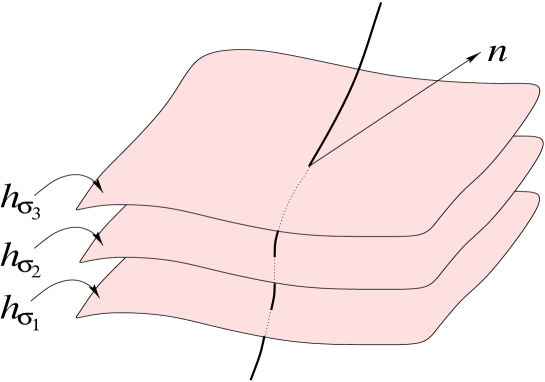
Figure 1: Foliation of spacetime: Each hypersurface $h_{\sigma}$ represents, at a time $\sigma$, the 3-dimensional space of our perception one dimension of which is suppressed in the figure. The positive time direction runs upwards.

We assume that this continuum admits a foliation into a succession of different leaves or hypersurfaces $h$. Accordingly, spacetime looks like a pile of leaves which can be numbered by a monotonically increasing (time) parameter $\sigma$. A leaf $h_{\sigma}$ is defined by $\sigma(x^{i})={const}$. It represents, at a certain time $\sigma$, the ordinary 3-dimensional space surrounding us (in Fig.1 it is 2-dimensional, since one dimension is suppressed).

At any given point in $h_{\sigma}$, we can introduce the covector $k_{i}:=\partial_{i}\sigma$ and a 4-vector $n=(n^{i})$ $=(n^{0},n^{1},n^{2},n^{3})=(n^{0},n^{a})$ such that $n$ is normalized according to

$$n^{i}\,k_{i}=n^{i}\partial_{i}\sigma=1\,.$$ (1)

Here $a,b\dots=1,2,3$ and $i,j\dots=0,1,2,3$. Furthermore, summation over repeated indices is always understood. The vector $n^{i}$ is “normal” to the leaf $h_{\sigma}$, whereas the covector $k_{i}$ is tangential to it.

With the pair $(n,k)$ we can construct projectors which decompose all tensor quantities into longitudinal  and transversal  constituents with respect to the vector $n$, see Fig.2. Indeed, the matrices

$$L^{i}{}_{j}:=n^{i}\,k_{j}\quad{\rm and}\quad T^{i}{}_{j}:=\delta^{i}_{j}-n^{i}\,k_{j}\quad{\rm with}\quad L^{i}{}_{j}+T^{i}{}_{j}=\delta^{i}_{j}\,,$$ (2)

represent projection operators, i.e.

$$L^{i}{}_{j}\,L^{j}{}_{k}=L^{i}{}_{k}\,,\quad T^{i}{}_{j}\,T^{j}{}_{k}=T^{i}{}_{k}\,,\quad L^{i}{}_{j}\,T^{j}{}_{k}=T^{i}{}_{j}\,L^{j}{}_{k}=0\,.$$ (3)

Taking an arbitrary covector $U_{i}$, we now can write it as

$$U_{i}={}^{\bot}\!U_{i}+\underline{U}_{i}\,,\quad{\rm where}\quad{}^{\bot}U_{i}:=L^{j}{}_{i}\,U_{j}\quad{\rm and}\quad\underline{U}_{i}:=T^{j}{}_{i}\,U_{j}\,.$$ (4)

Obviously ${}^{\bot}U_{i}$ describes the longitudinal component of the covector and $\underline{U}_{i}$ its transversal component, with $n^{i}\,\underline{U}_{i}=0$. Analogously, for an arbitrary vector $V^{i}$, we can write

$$V^{i}={}^{\bot}\!V^{i}+\underline{V}^{i}\,,\quad{\rm where}\quad{}^{\bot}V^{i}:=L^{i}{}_{j}\,V^{j}\quad{\rm and}\quad\underline{V}^{i}:=T^{i}{}_{j}\,V^{j}\,.$$ (5)

Its transversal component $\underline{V}^{i}$ fulfills $\underline{V}^{i}\,k_{i}=0$. This pattern can be straightforwardly generalized to all tensorial quantities of spacetime.

For simplicity, we confine our attention to the particular case when “adapted” coordinates $x^{i}=(\sigma,x^{a})$ are used and when the “spatial” components of $n$ vanish, i.e., $n^{i}=(1,0,0,0)$. In that case, we simply have $k_{i}=\partial_{i}\sigma=(1,0,0,0)$ and hence $\sigma$ can be treated as a formal “time” coordinate.

3 Conservation of electric charge (axiom 1)

The conservation of electric charge was already recognized as fundamental law during the time of Franklin (around 1750) well before Coulomb discovered the force law in 1785. Nowadays, at a time, at which one can catch single electrons and single protons in traps and can count them individually, we are more sure than ever that electric charge conservation is a valid fundamental law of nature. Therefore matter carries as a primary quality something called electric charge which only occurs in positive or negative units of an elementary charge $e$ (or, in the case of quarks, in $1/3$th of it) and which can be counted in principle. Thus it is justified to introduce the physical dimension of charge $q$ as a new and independent concept. Ideally one should measure a charge in units of $e/3$. However, for practical reasons, the SI-unit C (Coulomb) is used in laboratory physics.

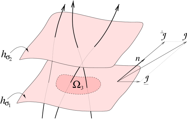
Figure 2: World lines, decomposition of the electric current into the piece ${}^{\bot}{\cal J}$ longitudinal to $n$ and the transversal piece $\underline{{\cal J}}$, global conservation of charge.

Two remarks are in order: Charge is an additive (or extensive) quantity that characterizes the source of the electromagnetic field. It is prior to the notion of the electric field strength. Therefore it is not reasonable to measure, as is done in the CGS-system of units, the additive quantity charge in terms of the unit of force by applying Coulomb’s law. Coulomb’s law has no direct relation to charge conservation. Secondly, in the SI-system, for reasons of better realization, the Ampere $A$ as current is chosen as the new fundamental unit rather than the Coulomb. We have $C=A\,s$ ($s=$ second).

As a preliminary step, let us remind ourselves that, in a 4-dimensional picture, the motion of a point particle is described, as in Fig.2, by a curve in spacetime, by a so-called worldline. The tangent vectors of this worldline represent the 4-velocity of the particle.

If we mark a 3-dimensional volume $\Omega_{3}$ which belong to a certain hypersurface $h_{\sigma}$, then the total electric charge inside $\Omega_{3}$ is

$$Q=\int\limits_{\Omega_{3}\subset h_{\sigma}}\rho\,dx^{1}dx^{2}dx^{3}\,,$$ (6)

with $\rho$ as the electric charge density. The total charge in space, which we find by integration over the whole of space, i.e., by letting $\Omega_{3}\rightarrow h_{\sigma}$, is globally conserved. Therefore the integral in (6) over each hypersurface $h_{\sigma_{1}},h_{\sigma_{2}},\dots$ keeps the same value.

The local conservation of charge, see Fig.3, translates into the following fact: If a number of worldlines of particles with one elementary charge enter a prescribed but arbitrary 4-dimensional volume $\Omega_{4}$, then, in classical physics, the same number has to leave the volume. If we count the entering worldlines as negative and the leaving ones as positive (in conformity with the direction of their normal vectors), then the (3-dimensional) surface integral over the number of worldlines has to vanish.

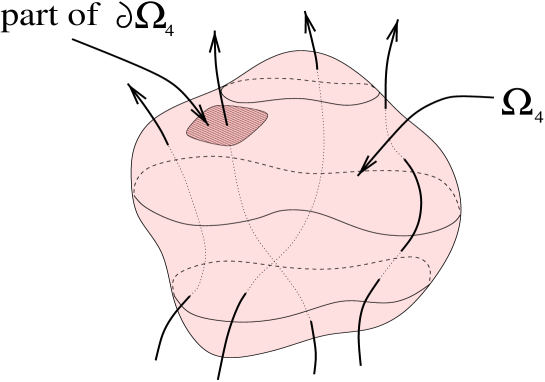
Figure 3: Local conservation of charge: Each worldline of a charged particle that enters the finite 4-volume $\Omega_{4}$ via its boundary $\partial\Omega_{4}$ has also to leave $\Omega_{4}$.

Now, the natural extensive quantities to be integrated over a 3-dimensional hypersurface are vector densities, see the appendix. Accordingly, in nature there should exist a 4-vector density ${\cal J}^{i}$ with 4 independent components which measures the charge piercing through an arbitrary 3-dimensional hypersurface. Therefore, it generalizes in a consistent 4-dimensional formalism the familiar concepts of charge density $\rho$ and current density $j^{a}$. The axiom of local charge conservation then reads

$$\int\limits_{\partial\Omega_{4}}{\cal J}^{i}\,d^{3}S_{i}=0\,,$$ (7)

where the integral is taken over the (3-dimensional) boundary of an arbitrary 4-dimensional volume of spacetime, with $d^{3}S_{i}$ being the 3-surface element, as defined in the appendix.

If we apply Stokes’ theorem, then we can transform the 3-surface integral in (7) into a 4-volume integral:

$$\int\limits_{\Omega_{4}}(\partial_{i}{\cal J}^{i})\,d^{4}S=0\,.$$ (8)

Since this is valid for an arbitrary 4-volume $\Omega_{4}$, we find the local version of the charge conservation as

$$\partial_{i}{\cal J}^{i}=0\,.$$ (9)

In this form, the law of conservation of charge is valid in arbitrary coordinates.

If one defines a particular foliation, then one can rewrite (9) in terms of decomposed quantities that are longitudinal and transversal to the corresponding normal vector $n$. The 4-vector density ${\cal J}^{i}$ decomposes as

$${\cal J}^{i}={}^{\bot}{\cal J}^{i}+\underline{\cal J}^{i}\,.$$ (10)

When adapted coordinates are used, the decomposition procedure simplifies and allows to define the 3-dimensional densities of charge $\rho$ and of current $j^{a}$ as

$$\rho:={}^{\bot}{\cal J}^{0}={\cal J}^{0},\qquad j^{a}:=\underline{\cal J}^{a}={\cal J}^{a}.$$ (11)

With this, one can rewrite the definition of charge (6) in an explicitly coordinate invariant form

$$Q=\int\limits_{\Omega_{3}\subset h_{\sigma}}{\cal J}^{i}\,d^{3}S_{i}\,,$$ (12)

since on $h_{\sigma}$ we have $d^{3}S_{0}=dx^{1}dx^{2}dx^{3}$ and $d^{3}S_{a}=0$. Furthermore, Eq.(9) can be rewritten in (1+3)-form as the more familiar continuity equation

$$\partial_{\sigma}\rho+\partial_{a}j^{a}=0\,.$$ (13)

The charge $Q$ in (12) has the absolute dimension $q$. The 4-current is a density in spacetime, and we have $[{\cal J}]=q/(t\,l^{3})$. Thus the components carry the dimensions $[\rho]=[{\cal J}^{0}]=q/l^{3}\stackrel{{\scriptstyle{\rm SI}}}{{=}}C/m^{3}$ and $[j^{a}]=[{\cal J}^{a}]=q/(t\,l^{2})\stackrel{{\scriptstyle{\rm SI}}}{{=}}A/m^{2}$.

4 The inhomogeneous Maxwell equations as consequence

Because of axiom 1 and according to a theorem of de Rham, see [5], the electric current density from (7) or (9) can be represented as a “divergence” of the electromagnetic excitation:

$${\cal J}^{i}=\partial_{j}\,{\cal H}^{ij}\,,\qquad{\cal H}^{ij}=-{\cal H}^{ji}\,.$$ (14)

The excitation ${\cal H}^{ij}$ is a contravariant antisymmetric tensor density and has 6 independent components. One can verify that, due to the antisymmetry of ${\cal H}^{ij}$, the conservation law is automatically fulfilled, i.e., $\partial_{i}{\cal J}^{i}=\partial_{i}\partial_{j}{\cal H}^{ij}=0$.

The 4-dimensional set (14) represents the inhomogeneous Maxwell equations. They surface here in a very natural way as a result of charge conservation. Charge conservation should not be looked at as a consequence of the inhomogeneous Maxwell equations, but rather the other way round, as shown in this tutorial. Of course, ${\cal H}^{ij}$ is not yet fully determined since

$$\tilde{{\cal H}}^{ij}={\cal H}^{ij}+\epsilon^{ijkl}\,\partial_{k}\psi_{l}$$ (15)

also satisfies (14) for an arbitrary covector field $\psi_{i}$.

The $(1+3)$-decomposition of ${\cal H}^{ij}$ is obtained similarly to the decomposition of the current (10):

$${\cal H}^{ij}={}^{\bot}{\cal H}^{ij}+\underline{{\cal H}}^{ij}.$$ (16)

The nontrivial components of the longitudinal and transversal parts read

$${\cal H}^{0a}={}^{\bot}{\cal H}^{0a}={\cal D}^{a},\qquad{\cal H}^{ab}=\underline{{\cal H}}^{ab}=\epsilon^{abc}\,{H}_{c}\,,$$ (17)

with the electric excitation ${\cal D}^{a}$ (historical name: “dielectric displacement”) and the magnetic excitation ${H}_{a}$ (“magnetic field”). Here $\epsilon^{abc}$ is the totally antisymmetric 3-dimensional Levi-Civita tensor density with $\epsilon^{123}=1$.

If we substitute the decompositions (10) and (16) into (14), we recover the 3-dimensional form of the inhomogeneous Maxwell equations,

$$\partial_{a}{\cal D}^{a}=\rho,\qquad\epsilon^{abc}\partial_{b}H_{c}-\partial_{\sigma}{\cal D}^{a}=j^{a}\,,$$ (18)

or, in symbolic notation,

$${\rm div}\,{\cal D}=\rho,\qquad{\rm curl}\,{{H}}-\dot{{\cal D}}=j\,.$$ (19)

Since electric charge conservation is valid in microphysics, the corresponding Maxwell equations (18) or (19) are also microphysical equations and with them the excitations ${\cal D}^{a}$ and ${H}_{a}$ are microphysical quantities likewise – in contrast to what is stated in most textbooks, see [8] and [12], compare also [2], e.g..

From (18) we can immediately read off $[{\cal D}^{a}]=[l\,\rho]=q/l^{2}\stackrel{{\scriptstyle\rm SI}}{{=}}C/m^{3}$ and $[H_{a}]=[l\,j^{a}]=q/(t\,l)\stackrel{{\scriptstyle\rm SI}}{{=}}A/m$. Before we ever talked about forces on charges, charge conservation alone gave us the inhomogeneous Maxwell equations including the appropriate dimensions for the excitations ${\cal D}^{a}$ and $H_{a}$.

Under the assumption that ${\cal D}^{a}$ vanishes inside an ideal electric conductor, one can get rid of the indeterminacy of ${\cal D}^{a}$, as spelled out in (15), and we can measure ${\cal D}^{a}$ by means of two identical conducting plates (“Maxwellian double plates”) which touch each other and which are separated in the ${\cal D}^{a}$-field to be measured. The charge on one plate is then measured. Analogous remarks apply to $H_{a}$. Accordingly, the excitations do have a direct operational significance.

5 Force and field strengths (axiom 2)

By now we have exhausted the information contained in the axiom 1 of charge conservation. We have to introduce new concepts in order to complete the fundamental structure of Maxwell’s theory. Whereas the excitation ${\cal H}=({\cal D}^{a},\,{H}_{a})$ is linked to the charge current ${\cal J}=(\rho,\,j^{a})$, the electric and magnetic field strengths are usually introduced as forces acting on unit charges at rest or in motion, respectively. In the purely electric case with a test charge $q$, we have in terms of components

$${F}_{a}\sim q\,E_{a}\,,$$ (20)

with ${F}$ as force and $E$ as electric field covector.

Let us take a (delta-function-like) test charge current ${\cal J}=(\rho,\,j^{a})$ centered around a point with spatial coordinates $x^{a}$. Generalizing (20), the simplest relativistic ansatz for defining the electromagnetic field reads:

$${\rm force\>\>density}\quad\sim\quad{\rm field\>\>strength}\times{\rm charge\>\>current\>\>density}\,.$$ (21)

We know from Lagrangian mechanics that the force $\sim\partial L/\partial x^{i}$ is represented by a covector with the absolute dimension of action $\hbar$ (here $\hbar$ is not the Planck constant but rather only denotes its dimension). Accordingly, with the covectorial force density $f_{i}$, the ansatz (21) can be made more precise as axiom 2:

$$f_{i}=F_{ij}\,{\cal J}^{j}\,,\qquad F_{ij}=-F_{ji}\,.$$ (22)

The newly introduced covariant 2nd-rank 4-tensor $F_{ij}$ is the electromagnetic field strength. The force density $f_{i}$ was postulated to be normal to the current, $f_{i}\,{\cal J}^{i}=0$. Thus the antisymmetry of the electromagnetic field strength is found, i.e., $F_{ij}$ depends on 6 independent components. We know the notion of force from mechanics, the current density we know from axiom 1. Accordingly, axiom 2 is to be understood as an operational definition of the electromagnetic field strength $F_{ij}$.

With the decomposition

$$F_{ij}={}^{\bot}F_{ij}+\underline{F}_{ij}\,,$$ (23)

we find the identifications for the electric field strength $E_{a}$ and the magnetic field strength ${\cal B}^{a}$ (historical names: “magnetic induction” or “magnetic flux density”):

$$F_{a0}={}^{\bot}F_{a0}=E_{a},\qquad F_{ab}=\underline{F}_{ab}=\epsilon_{abc}\,{\cal B}^{c}.$$ (24)

These identifications are reasonable since for the spatial components of (22) we recover the Lorentz force density and, for the static case, Eq.(20):

$$f_{a}=F_{aj}\,{\cal J}^{j}=F_{a0}\,{\cal J}^{0}+F_{ab}\,{\cal J}^{b}=\rho\,E_{a}+\epsilon_{abc}\,j^{b}\,{\cal B}^{c}\,.$$ (25)

Symbolically, we have

$$f=\rho\,E+j\times{\cal B}\,.$$ (26)

The time component of (22) represents the electromagnetic power density:

$$f_{0}=F_{0a}\,{\cal J}^{a}=-E_{a}\,j^{a}\,.$$ (27)

6 Conservation of magnetic flux (axiom 3)

Axiom 2 on the Lorentz force gave us a new quantity, the electromagnetic field strength with the dimension $[F]=action/charge=\hbar/q=:\phi$, with $\phi=work\times time/charge=voltage\times time\stackrel{{\scriptstyle\rm SI}}{{=}}Vs=W\!b$. Here $W\!b$ is the abbreviation for Weber. Thus its components carry the following dimensions: $[E_{a}]=[F_{a0}]=\phi/(t\,l)\stackrel{{\scriptstyle\rm SI}}{{=}}V/m$ and $[{\cal B}^{c}]=[F_{ab}]=\phi/l^{2}\stackrel{{\scriptstyle\rm SI}}{{=}}W\!b/m^{2}=T$ (for Tesla).

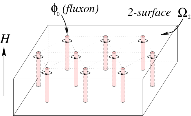
Figure 4: Sketch of an Abrikosov lattice in a type II superconductor in 3-dimensional space. In contrast to all the other figures, this is not an image of 4-dimensional spacetime.

We are in need of an experimentally established law that relates to $F$. And we would prefer, as in the case of the electric charge, to recur to a counting procedure. What else can we count in relation to the electromagnetic field? Certainly magnetic flux lines in the interior of a type II superconductor which is exposed to a sufficiently strong magnetic field. And these flux lines are quantized. In fact, they can order in a 2-dimensional triangular Abrikosov lattice, see Fig.4. These flux lines carry a unit of magnetic flux, a so-called flux quantum or fluxon with $\Phi_{0}=h/(2e)=2.07\times 10^{-15}\,W\!b\,,$ see Tinkham [17]; here $h$ is the Planck constant and $e$ the elementary charge. These flux lines can move, via its surface, in or out of the superconductor, but they cannot vanish (unless two lines with different sign collide) or spontaneously come into existence. In other words, there is a strong experimental evidence that magnetic flux is a conserved quantity.

The number $2$ in the relation $\Phi_{0}=h/(2e)$ is due to the fact that the Cooper pairs in a superconductor consist of 2 electrons. Moreover, outside a superconductor the magnetic flux is not quantized, i.e., we cannot count the flux lines there with the same ease that we could use inside. Nevertheless, as we shall see, experiments clearly show that the magnetic flux is conserved also there.

As we can take from Fig.4, the magnetic flux should be defined as a 2-dimensional spatial integral. These flux lines are additive and we have

$$\Phi=\int\limits_{\Omega_{2}\subset h_{\sigma}}{\cal B}^{a}\,d^{2}S_{a}\,.$$ (28)

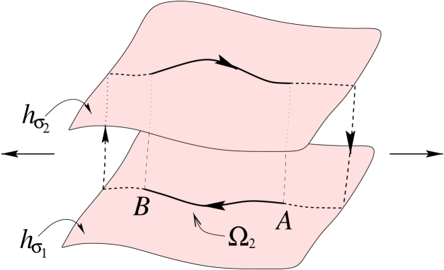
Figure 5: Magnetic flux in spacetime: The magnetic field ${\cal B}^{a}$, if integrated over the interval $[A,B]$, represents, at time $\sigma_{1}$, the magnetic flux piercing through this 2-dimensional integration domain.

Here ${\cal B}^{a}$ is the magnetic field strength and $d^{2}S_{a}$ the spatial 2-surface element. This definition of the magnetic flux should be compared with the definition (6) of the charge. Here, in (28), we integrate only over $2$ dimensions rather than over $3$ dimensions, as in the case of the charge in (6). Thus in a spacetime picture in which one space dimension is suppressed, see Fig.5, our magnetic flux integral looks like an integral over a finite interval $[A,B]$ embedded into the hypersurface $h_{\sigma_{1}}$.

Now we are going to argue again as in Sec.3. If $\Omega_{2}\rightarrow\infty$, i.e., if we integrate over an infinite spatial 2-surface ($A\rightarrow+\infty,\,B\rightarrow-\infty$), then the total magnetic flux at time $\sigma_{1}$ is given by (28). If we propagate that interval into the (coordinate) future, see the interval on the hypersurface $h_{\sigma_{2}}$, then magnetic flux conservation requires the constancy of the integral $\Phi$. In other words, if we orient the integration domain suitably, the loop integral, the domain of which is drawn in Fig.5, has to vanish since no flux is supposed to leak out along the dotted “vertical” domains at spatial infinity.

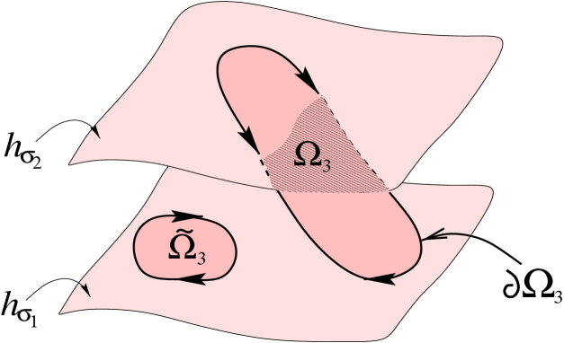
Figure 6: Conservation of magnetic flux in spacetime: Consider the arbitrary 3-dimensional integration domain $\Omega_{3}$. The integral vanishes of the field strength $F_{ij}$ over the 2-dimensional boundary $\partial\Omega_{3}$ of the 3-dimensional domain $\Omega_{3}$. The analogous is true for the flux integral over $\partial\tilde{\Omega}_{3}$.

Analogously as we did in the case of charge conservation, we want to formulate a corresponding local conservation law in an explicitly covariant way. We saw that the global conservation of magnetic flux is expressed as the vanishing of the integral of ${\cal B}$ over the particular 2-dimensional loop in Fig.5. In a 4-dimensional covariant formalism, the natural intensive objects to be integrated over a 2-dimensional region are second order antisymmetric covariant tensors, see the appendix. The magnetic field strength ${\cal B}$ is just a piece of the electromagnetic field strength $F$. Thus, it is clear that the natural local generalization of the magnetic flux conservation, our axiom 3, is

$$\int\limits_{\partial\Omega_{3}}\frac{1}{2}\,F_{ij}\,d^{2}S^{ij}=0\,,$$ (29)

where the integral is taken over the boundary of an arbitrary 3-dimensional hypersurface of spacetime, as is sketched in Fig.6. We apply Stokes’ theorem

$$\int\limits_{\Omega_{3}}\epsilon^{ijkl}\partial_{[j}\,F_{kl]}\,d^{3}S_{i}=0\,,$$ (30)

and, since the volume is arbitrary, we have the local version of magnetic flux conservation as

$$\partial_{[i}F_{jk]}=0.$$ (31)

We substitute the decomposition (23) into (31). Then we find the homogeneous Maxwell equations,

$$\partial_{a}{\cal B}^{a}=0\,,\qquad\epsilon^{abc}\partial_{b}E_{c}+\partial_{\sigma}{\cal B}^{a}=0\,$$ (32)

or, symbolically,

$${\rm div}\,{\cal B}=0\,,\qquad{\rm curl}\,E+\dot{{\cal B}}=0\,.$$ (33)

Thus both, the sourcelessness of ${\cal B}^{a}$ and the Faraday induction law follow from magnetic flux conservation. Both laws are experimentally very well verified and, in turn, strongly support the axiom of the conservation of the magnetic flux.

The recognition that Maxwell’s theory, besides on charge conservation, is based on magnetic flux conservation, sheds new light on the possible existence of magnetic monopoles. First of all, careful search for them has not lead to any signature of their possible existence, see [6]. Furthermore, magnetic flux conservation would be violated if we postulated the existence of a current on the right hand side of (31). Now, Eq.(9) is the analog of (31), at least in our axiomatic set-up. Why should we believe in charge conservation any longer if we gave up magnetic flux conservation? Accordingly, we assume – in contrast to most elementary particle physicists, see Cheng & Li [3] – that in Maxwell’s theory proper there is no place for a magnetic current on the right hand side of (31).

7 Constitutive law (axiom 4)

The Maxwell equations (14) and (31) or, in the decomposed version, (19) and (33), respectively, encompass altogether 6 partial differential equations with a first order time derivative (the 2 remaining equations can be understood as constraints to the initial configuration). Since excitations and field strengths add up to $6+6=12$ independent components, certainly the Maxwellian set is underdetermined with respect to the time propagation of the electromagnetic field. What we clearly need is a relation between the excitations and the field strengths. As we will see, these so-called constitutive equations require additional knowledge about the properties of spacetime whereas the Maxwell equations, as derived so far, are of universal validity as long as classical physics is a valid approximation. In particular, in the Riemannian space of Einstein’s gravitational theory the Maxwell equations look just the same as in (14) and (31). There is no adaptation needed of any kind, see [11].

If we investigate macroscopic matter, one has to derive from the microscopic Maxwell equations by statistical procedures the macroscopic Maxwell equations. They are expected to have the same structure as the microscopic ones. But let us stay, for the time being, on the microscopic level.

Then we can make an attempt with a linear constitutive relation between ${\cal H}^{ij}$ and $F_{kl}$,

$${\cal H}^{ij}=\frac{1}{2}\,\tilde{\chi}^{ijkl}\,F_{kl}=\frac{1}{2}\,f{\chi}^{ijkl}\,F_{kl}\,,$$ (34)

with the tensor density ${\chi}^{ijkl}$ that is characteristic for the spacetime under consideration. We require $[{\chi}]=1$, i.e., for the dimensionfull scalar factor factor $f$ we have $[f]=q/\phi=q^{2}/h\stackrel{{\scriptstyle\rm SI}}{{=}}C/(Vs)=A/V=1/\Omega$. The dimensionless “modulus” ${\chi}^{ijkl}$, because of the antisymmetries of ${\cal H}^{ij}$ and $F_{kl}$, obeys

$${\chi}^{ijkl}=-{\chi}^{jikl}=-{\chi}^{ijlk}\,.$$ (35)

Moreover, if we assume the existence of a Lagrangian density for the electromagnetic field ${\cal L}\sim{\cal H}^{ij}F_{ij}$, then we have additionally the symmetries

$${\chi}^{ijkl}={\chi}^{klij}\,,\qquad{\chi}^{[ijkl]}=0\,.$$ (36)

The vanishing of the totally antisymmetric part comes about since the corresponding Euler-Lagrange derivative of ${\cal L}$ with respect to the 4-potential $A_{i}$ identically vanishes; here $F_{ij}=2\partial_{[i}A_{j]}$. For ${\chi}^{ijkl}$, this leaves 20 independent components. One can take such moduli, if applied on a macrophysical scale, for describing the electromagnetic properties of anisotropic crystals, e.g.. Then also non-linear (for ferromagnetism) and spatially non-local constitutive laws are in use.

The simplest linear law is expected to be valid in vacuum. Classically, the vacuum of spacetime is described by its metric tensor $g^{ij}=g^{ji}$ that determines the temporal and spatial distances of neighboring events. Considering the symmetry properties of the density ${\chi}^{ijkl}$, the only ansatz possible, up to an arbitrary constant, seems to be

$${\chi}^{ijkl}=\sqrt{-\det g_{mn}}\,\left(g^{ik}g^{jl}-g^{jk}g^{il}\right)\,.$$ (37)

Note that ${\chi}^{ijkl}$ is invariant under a rescaling of the metric $g_{ij}\rightarrow\Omega^{2}g_{ij}$, with an arbitrary function $\Omega(x^{i})$. Using this freedom, we can always normalize the determinant of the metric to 1.

As an example, let us consider the flat spacetime metric of a Minkowski space in Minkowskian coordinates,

$$\eta^{ij}={{\sqrt{c}}}\left(\begin{array}[]{crrr}c^{-2}&0&0&0\\ 0&-1&0&0\\ 0&0&-1&0\\ 0&0&0&-1\end{array}\right).$$ (38)

If we substitute (38) into (37) and, in turn, Eq.(37) and $f=\sqrt{\varepsilon_{0}/\mu_{0}}$ into (34), then we eventually find the well-known vacuum (“Lorentz aether”) relations,

$${\cal H}^{ij}=\sqrt{\frac{\varepsilon_{0}}{\mu_{0}}}\eta^{ik}\eta^{jl}\,F_{kl}\qquad{\rm or}\qquad{\cal D}=\varepsilon_{0}\,E\,,\quad H=(1/\mu_{0})\,{\cal B}\,.$$ (39)

The law (39) converts Maxwell’s equations, for vacuum, into a system of differential equations with a well-determined initial value problem.

Acknowledgments: We are grateful to Marc Toussaint for discussions on magnetic monopoles. G.F.R. would like to thank the German Academic Exchange Service DAAD for a graduate fellowship (Kennziffer A/98/00829).

Appendix A Four-dimensional calculus without metric and integrals

In a 4-dimensional space, in which arbitrary coordinates $x^{i}$ are used, with $i=0,1,2,3$, one can define derivatives and integrals of suitable antisymmetric covariant tensors and antisymmetric contravariant tensor densities without the need of a metric. The tensors are used for representing intensive quantities (how strong?), the tensor densities for extensive (additive) quantities (how much?). The natural formalism for defining integrals in a coordinate invariant way is exterior calculus, see Frankel [5]. However, we will use here tensor calculus, see Schouten [14] and also Schrödinger [15], which is more widely known under physicists and engineers.

Integration over 4-dimensional regions – scalar densities

Consider a certain 4-dimensional region $\Omega_{4}$. Then a integral over $\Omega_{4}$ is of the form

$$\int_{\Omega_{4}}{\cal A}\,d^{4}S\,,$$ (40)

where $d^{4}S:=dx^{0}dx^{1}dx^{2}dx^{3}$ is the 4-volume element which is a scalar density of weight $-1$. We want this integral to be a scalar, i.e., that its value does not depend on the particular coordinates we use. Then the integrand ${\cal A}$ has to be a scalar density of weight $+1$. In other words, when using the tensor formalism, the natural quantity required to formulate an invariant integral over a 4-dimensional region is a scalar density of weight $+1$.

Integration over 3-dimensional regions – vector densities

Now we want to define invariant integrals over some 3-dimensional hypersurface $\Omega_{3}$ in a four-dimensional space which can be defined by the parameterization $x^{i}=x^{i}(y^{a})$, $a,b,c=1,2,3$, where $y^{a}$ are also arbitrary coordinates on $\Omega_{3}$. Then we call

$$d^{3}S_{i}:=\frac{1}{3!}\,\epsilon_{ijkl}\,\frac{\partial x^{j}}{\partial y^{a}}\frac{\partial x^{k}}{\partial y^{b}}\frac{\partial x^{l}}{\partial y^{c}}\,\epsilon^{abc}\,dy^{1}dy^{2}dy^{3}$$ (41)

the 3-surface element on $\Omega_{3}$. This quantity is constructed by using only objects that can be defined in a general 4-dimensional space without metric or connection. It can be constructed as soon as we specify the parameterization of $\Omega_{3}$. Here $\epsilon_{ijkl}$ is the 4-dimensional Levi-Civita tensor density of weight $-1$ and $\epsilon^{abc}$ the 3-dimensional Levi-Civita tensor density of weight $+1$ on $\Omega_{3}$. Furthermore, this hypersurface element turns out to be a covector density of weight $-1$ with respect to 4-dimensional coordinate transformation. With this integration element to our disposal, the natural form of an invariant integral over $\Omega_{3}$ is

$$\int_{\Omega_{3}}{\cal A}^{i}d^{3}S_{i}\,.$$ (42)

Therefore, the natural object to be integrated over $\Omega_{3}$ in order to obtain an invariant result is a vector density of weight $+1$.

Integration over 2-dimensional regions – covariant tensors or contravariant tensor densities

Analogously, we can parameterize a 2-dimensional region $\Omega_{2}$ by means of $x^{i}=x^{i}(z^{\alpha})$, $\alpha,\beta=1,2$, where $z^{\alpha}$ are arbitrary coordinates on $\Omega_{2}$. Then we can immediately construct the following 2-surface element

$$d^{2}S_{ij}:=\frac{1}{2}\,\epsilon_{ijkl}\,\frac{\partial x^{k}}{\partial z^{\alpha}}\frac{\partial x^{l}}{\partial z^{\beta}}\,\epsilon^{\alpha\beta}\,dz^{1}dz^{2},$$ (43)

where $\epsilon^{\alpha\beta}$ is the Levi-Civita density of weight $+1$ on $\Omega_{2}$. This surface element is an antisymmetric second order covariant tensor density of weight $-1$. Then an invariant integral is naturally defined as

$$\int_{\Omega_{2}}\frac{1}{2}{\cal A}^{ij}\,d^{2}S_{ij}\,,$$ (44)

with ${\cal A}^{ij}$ being an antisymmetric second order contravariant tensor density of weight $+1$.

Alternatively, one can write the same integral in terms on an antisymmetric second order covariant tensor $A_{ij}:=\frac{1}{2}\epsilon_{ijkl}{\cal A}^{kl}$ and an antisymmetric second order contravariant surface element

$$d^{2}S^{ij}:=\frac{\partial x^{k}}{\partial z^{\alpha}}\frac{\partial x^{l}}{\partial z^{\beta}}\epsilon^{\alpha\beta}\,dz^{1}dz^{2}\,,$$ (45)

such that

$$\int_{\Omega_{2}}\frac{1}{2}{\cal A}^{ij}\,d^{2}S_{ij}=\int_{\Omega_{2}}\frac{1}{2}A_{ij}\,d^{2}S^{ij}\,.$$ (46)

Since extensive quantities are represented by densities, we would take the first integral for them, whereas for intensive quantities the second integral should be used. Analogous considerations can be applied to (40) and (42).

Stokes’ theorem

Stokes’ theorem gives us as particular cases the following integral identities (see [14] p.67 et seq.):

$$\int_{\Omega_{4}}(\partial_{i}{\cal J}^{i})\,d^{4}S=\int_{\partial\Omega_{4}}{\cal J}^{i}\,d^{3}S_{i}\,,$$ (47)

$$\int_{\Omega_{3}}(\partial_{j}{\cal H}^{ij})\,d^{3}S_{i}=\int_{\partial\Omega_{3}}\frac{1}{2}\,{\cal H}^{ij}\,d^{2}S_{ij}\,.$$ (48)

Appendix B Decomposition of totally antisymmetric tensors into longitudinal and transversal pieces

Here we provide the decomposition formulas for totally antisymmetric covariant and contravariant tensors, which are the natural generalization of the decomposition of vectors and covectors.

We start by considering an antisymmetric covariant tensor of rank $p$, namely $U_{i_{1}\dots i_{p}}$. Its longitudinal and transversal components are given by

$${}^{\bot}U_{i_{1}\dots i_{p}}=p\ L^{m}_{\ [i_{1}|}U_{m|i_{2}\dots i_{p}]}\,,\qquad\underline{U}_{i_{1}\dots i_{p}}=(p+1)L^{m}_{\ [m}U_{i_{1}\dots i_{p}]}\,,$$ (49)

where $k_{i}:=\partial_{i}\sigma$, and $L^{i}_{\ j}:=n^{i}k_{j}$. They fulfill the following properties:

$$n^{i_{1}}\underline{U}_{i_{1}\dots i_{p}}=0\,,\qquad n^{i_{1}}{}^{\bot}U_{i_{1}\dots i_{p}}=n^{i_{1}}U_{i_{1}\dots i_{p}}\,.$$ (50)

For $p=1,2,3,4$ we can explicitly write:

$p$	quantity	definition	explicitly
$1$	${}^{\bot}U_{i}$	$L^{m}_{\ i}U_{m}$	$n^{m}k_{i}U_{m}$
$2$	${}^{\bot}U_{ij}$	$2L^{m}_{\ [i|}U_{m|j]}$	$n^{m}\left(k_{i}U_{mj}-k_{j}U_{mi}\right)$
$3$	${}^{\bot}U_{ijk}$	$3L^{m}_{\ [i|}U_{m|jk]}$	$n^{m}\left(k_{i}U_{mjk}+k_{j}U_{mki}+k_{k}U_{mij}\right)$
$4$	${}^{\bot}U_{ijkl}$	$4L^{m}_{\ [i|}U_{m|jkl]}$	$n^{m}\left(k_{i}U_{mjkl}-k_{j}U_{mkli}+k_{k}U_{mlij}-k_{l}U_{mijk}\right)$

Now we turn to $V^{i_{1}\dots i_{p}}$, an antisymmetric contravariant tensors of rank $p$. We define the decomposition as

$${}^{\bot}V^{i_{1}\dots i_{p}}=p\ L^{[i_{1}|}_{\ \ m}V^{m|i_{2}\dots i_{p}]}\,,\qquad\underline{V}^{i_{1}\dots i_{p}}=(p+1)L^{[m}_{\ \ m}V^{i_{1}\dots i_{p}]}\,.$$ (51)

They fulfill

$$k_{i_{1}}\underline{V}^{i_{1}\dots i_{p}}=0\,,\qquad k_{i_{1}}{}^{\bot}V^{i_{1}\dots i_{p}}=k_{i_{1}}V^{i_{1}\dots i_{p}}\,.$$ (52)

For $p=1,2,3,4$ we have the following explicit expressions for the longitudinal components:

$p$	quantity	definition	explicitly
$1$	${}^{\bot}V^{i}$	$L^{i}_{\ m}V^{m}$	$n^{i}k_{m}V^{m}$
$2$	${}^{\bot}V^{ij}$	$2L^{[i|}_{\ \ m}V^{m|j]}$	$k_{m}\left(n^{i}V^{mj}-n^{j}V^{mi}\right)$
$3$	${}^{\bot}V^{ijk}$	$3L^{[i|}_{\ \ m}V^{m|jk]}$	$k_{m}\left(n^{i}V^{mjk}+n^{j}V^{mki}+n^{k}V^{mij}\right)$
$4$	${}^{\bot}V^{ijkl}$	$4L^{[i|}_{\ \ m}V^{m|jkl]}$	$k_{m}\left(n^{i}V^{mjkl}-n^{j}V^{mkli}+n^{k}V^{mlij}-n^{l}V^{mijk}\right)$

An analogous scheme is valid for the corresponding densities.

References

- [1] F. Bopp, Prinzipien der Elektrodynamik. Z. Physik 169 (1962) 45-52.
- [2] R.G. Chambers, Units – B, H, D, and E. Am. J. Phys. 67 (1999) 468-469.
- [3] T. Cheng and L. Li, Theory of Elementary Particle Physics. Clarendon Press, Oxford (1984).
- [4] V.L. Fitch, The far side of sanity. Am. J. Phys. 67 (1999) 467.
- [5] T. Frankel, The Geometry of Physics – An Introduction. Cambridge University Press, Cambridge (1997).
- [6] Y.D. He, Search for a Dirac magnetic monopole in high energy nucleus-nucleus collisions. Phys. Rev. Lett. 79 (1997) 3134-3137.
- [7] F.W. Hehl, J. Lemke, and E.W. Mielke, Two Lectures on Fermions and Gravity, in Geometry and Theoretical Physics, Proceedings of Bad Honnef School, Feb. 1990, J. Debrus and A.C. Hirshfeld, eds.. Springer, Berlin (1991) pp. 56-140.
- [8] J.D. Jackson, Classical Electrodynamics. 3rd ed.. Wiley, New York (1998).
- [9] Y.N. Obukhov and F.W. Hehl, Space-time metric from linear electrodynamics. Phys. Lett. B458 (1999) 466-470.
- [10] E.J. Post, Formal Structure of Electromagnetics – General Covariance and Electromagnetics. North Holland, Amsterdam (1962) and Dover, Mineola, New York (1997).
- [11] R.A. Puntigam, C. Lämmerzahl and F.W. Hehl, Maxwell’s theory on a post-Riemannian spacetime and the equivalence principle. Class. Quantum Grav. 14 (1997) 1347-1356.
- [12] W. Raith, Bergmann–Schaefer, Lehrbuch der Experimentalphysik, Vol.2, Elektromagnetismus, 8th ed.. de Gruyter, Berlin (1999).
- [13] M. Schönberg, Electromagnetism and gravitation. Rivista Brasileira de Fisica 1 (1971) 91-122.
- [14] J.A. Schouten, Tensor Analysis for Physicists. 2nd ed.. Dover, Mineola, New York (1989).
- [15] E. Schrödinger, Space-Time Structure. Cambridge University Press, Cambridge (1954).
- [16] A. Sommerfeld, Elektrodynamik. Vorlesungen über Theoretische Physik, Band 3. Dietrisch’sche Verlagsbuchhandlung, Wiesbaden (1948).
- [17] M. Tinkham, Introduction to Superconductivity. 2nd ed.. McGraw-Hill, New York (1996).
- [18] M. Toussaint, A gauge theoretical view of the charge concept in Einstein gravity. Gen. Relat. Grav. J., to appear 1999/2000. Los Alamos Eprint Archive gr-qc/9907024.
- [19] C. Truesdell and R.A. Toupin, The Classical Field Theories. In Handbuch der Physik, Vol. III/1, S. Flügge ed.. Springer, Berlin (1960) pp. 226-793.
- [20] M.R. Zirnbauer, Elektrodynamik. Tex-script of a course in Theoretical Physics II (in German), July 1998 (Springer, Berlin, to be published).