Multiple resonance compensation for betraton coupling and its equivalence with matrix method

Abstract

Analyses of betatron coupling can be broadly divided into two categories: the matrix approach that decouples the single-turn matrix to reveal the normal modes and the hamiltonian approach that evaluates the coupling in terms of the action of resonances in perturbation theory. The latter is often regarded as being less exact but good for physical insight. The common opinion is that the correction of the two closest sum and difference resonances to the working point is sufficient to reduce the off-axis terms in the $4\times 4$ single-turn matrix, but this is only partially true. The reason for this is explained, and a method is developed that sums to infinity all coupling resonances and, in this way, obtains results equivalent to the matrix approach. The two approaches is discussed with reference to the dynamic aperture. Finally, the extension of the summation method to resonances of all orders is outlined and the relative importance of a single resonance compared to all resonances of a given order is analytically described as a function of the working point.

1	CERN PS/HP, 1211 Geneve 23, Switzerland
2	Dept. of Numerical Analysis and Computer Science, KTH,
	S-100 44 Stockholm, Sweden

1 Introduction

The example of linear betatron coupling will be used in the first instance to demonstrate the summation of the influences of all the resonances in a given family into a single driving term. It will then be shown that is in fact a general result that can be applied to all linear and non-linear resonances.
Analyses of betatron coupling can be broadly divided into two categories: the matrix approach [3], [4], [5] that decouples the single-turn matrix to reveal the normal modes and the hamiltonian approach [6], [7] that evaluates the coupling in terms of the action of resonances using a perturbation method. The latter is often regarded as being less exact but good for physical insight. The general belief is that the correction of the two closest sum and difference resonances to the working point should be sufficient to reduce the off-axis terms in the $4\times 4$ single-turn matrix, but in most cases this is not successful.

1.1 Matrix method for coupling compensation

The $4\times 4$ single-turn matrix in the presence of skew quadrupoles and/or solenoids is of the form

$${\bf T}=\left(\begin{array}[]{cc}M&n\\ \\ m&N\end{array}\right),$$ (1)

(where $M,n,m,N\in\Re^{2\times 2}$). Coupling compensation is achieved by setting the two $2\times 2$ matrices $n$ and $m$ to zero. Due to symplecticity and periodicity of $T$ only four free parameters (that is the strengths of four compensator units) are required. However, this compensation is only valid at the origin of ${\bf T}$.
A transformation can also be applied to the matrix ${\bf T}$ that decouples the linear motion, so making it possible to describe the beam in the whole machine with the well-known Courant and Snyder parametrisation in the transformed coordinates.

1.2 Classical hamiltonian method for coupling compensation

This method is based on the expansion in a Fourier series of the coupling perturbation term in the Hamiltonian. The standard procedure is to assume that the low-frequency components dominate the motion and that only the nearest sum and difference resonances therefore require compensation (single resonance compensation).
The essential difference between this and the matrix approach is:

$~{}~{}~{}\bullet$  The matrix method is exact while the hamiltonian method is approximate;
$~{}~{}~{}\bullet$  A coupling compensation made by the matrix method is only valid at one point in the ring whereas the hamiltonian method gives a global correction;
$~{}~{}~{}\bullet$  The matrix method leaves finite excitations in all resonances, including those closest to the working point, whereas the hamiltonian method leaves finite excitations only in the far resonances.

The reason for the two last points is that the matrix method includes all resonances automatically and combines them in such a way that the matrix is uncoupled at one point, while the hamiltonian method sets only the closest sum and difference resonances to zero. If the far resonances have little effect, then the two methods are virtually equivalent. This is however an uncommon situation.
The logical implication is that by finding a way to sum all the resonances, the classical hamiltonian method can be made to reproduce the results found with the matrix method. Once this is done, the natural questions are which of the two methods is the better for operation, and if the principle can be extended to higher orders.

The aims of this paper are the following:
$~{}~{}~{}\bullet$  To outline a summed resonance compensation procedure (taking into account both the low and high-frequency part of the perturbative Hamiltonian) for the case of linear coupling and to extend this result to the non-linear case (Section 2);
$~{}~{}~{}\bullet$  To analytically compare (Section 3) the single and summed resonance theories pointing out some general results that can be obtained using the analytical expression of the generalized driving term;
$~{}~{}~{}\bullet$  To numerically compare the single and the summed resonance compensations for the linear coupling (the latter is shown to be equivalent to the matrix compensation) using a 4D coupled Henon map [8] (Section 4);

2 Multiple resonance compensation for linear coupling

The starting point for this analysis is taken from [6], with the initial assumptions that:
$~{}~{}~{}\bullet$  the perturbative Hamiltonian is calculated at $\theta=0$. Since the origin is an arbitrary choice, this is not a restriction;
$~{}~{}~{}\bullet$  solenoid fields are absent. The presence of solenoid fields does not change the argument but by omitting them the resulting equations become more transparent. They will be added at the end.

The linear coupling compensation using the notation of [6] requires (without any approximation for removing the high frequency part):

$$\left\{\begin{array}[]{l}\displaystyle{\sum_{p=-\infty}^{+\infty}h^{(2)}_{1010-p}=0}~{}~{}~{}~{}~{}~{}~{}~{}\mbox{sum resonance}\\ \\ \displaystyle{\sum_{p=-\infty}^{+\infty}h^{(2)}_{1001-p}=0}~{}~{}~{}~{}~{}~{}~{}~{}\mbox{difference resonance}.\end{array}\right.$$ (2)

2.1 Detailed derivation for difference resonances

Consider first the treatment of the difference resonances and express (2) explicitly as

$$\sum_{p=-\infty}^{+\infty}h^{(2)}_{1001-p}\equiv C^{-}_{\infty}=\sum_{p=-\infty}^{\infty}\int_{0}^{2\pi}A(\theta)e^{\displaystyle{-i(Q_{x}-Q_{y}-p)\theta}}\mbox{d}~{}\theta$$ (3)

where

$$A(\theta)=\frac{1}{4\pi R}\sqrt{\beta_{x}(\theta)\beta_{y}(\theta)}e^{\displaystyle{i[\mu_{x}(\theta)-\mu_{y}(\theta)]}}k(\theta),$$ (4)

$$k(\theta)=\frac{R^{2}}{B\rho}\frac{\partial B_{x}}{\partial x},$$ (5)

$\theta=s/R$ is the coordinate along the ring, $Q_{x,y}$ are the horizontal and vertical tunes, $\mu_{x,y}$ are the horizontal and vertical phase advances, $\beta_{x,y}$ are the horizontal and vertical beta functions and $R$ is the radius of the ring.
Suppose $k(\theta)$ is different from zero and constant in $j$ short intervals (i.e. the regions occupied by the sources of coupling and by possible correctors) $[\theta_{i},\theta_{i}+\Delta\theta_{i}]$ in which $A(\theta)$ can be considered approximately constant (thin lens approximation) :

$$C^{-}_{\infty}=\sum_{i=1}^{j}(\Delta C^{-}_{\infty})_{i}.$$ (6)

Now define $\Delta^{-}\equiv Q_{x}-Q_{y}$ and compute $(\Delta C^{-}_{\infty})_{i}$, the contribution to $C^{-}_{\infty}$ from the $i-th$ sub-element,

$$(\Delta C^{-}_{\infty})_{i}=\sum_{p=-\infty}^{+\infty}\int_{\theta_{i}}^{\theta_{i}+\Delta\theta_{i}}A(\theta)e^{\displaystyle{-i[\Delta^{-}-p]\theta}}\mbox{d}\theta,$$ (7)

which, when integrated gives,

$$(\Delta C^{-}_{\infty})_{i}\simeq A(\theta_{i})\sum_{p=-\infty}^{+\infty}\frac{i}{\Delta^{-}-p}\left[e^{\displaystyle{-i[\Delta^{-}-p](\theta_{i}+\Delta\theta_{i})}}-e^{\displaystyle{-i[\Delta^{-}-p]\theta_{i}}}\right].$$ (8)

The summation can be redefined making use of the shift $[\Delta^{-}]$ (the closest integer to $\Delta^{-}$) so that $p=[\Delta^{-}]+k$ where $k$ is an integer. In the limit $(\Delta^{-}-[\Delta^{-}])\Delta\theta_{i}\ll 1$, the previous expression becomes

$$(\Delta C^{-}_{\infty})_{i} \simeq A(\theta_{i})e^{\displaystyle{-i(\Delta^{-}-[\Delta^{-}])\theta_{i}}}\sum_{k=-\infty}^{+\infty}\frac{i}{(\Delta^{-}-[\Delta^{-}])-k}\left[e^{\displaystyle{ik(\theta_{i}+\Delta\theta_{i})}}-e^{\displaystyle{ik\theta_{i}}}\right]=$$ (9)

$$= A(\theta_{i})e^{\displaystyle{-i(\Delta^{-}-[\Delta^{-}])\theta_{i}}}\sum_{k=-\infty}^{+\infty}\frac{1}{(\Delta^{-}-[\Delta^{-}])-k}\{\sin(k\theta_{i})-\sin[k(\theta_{i}+\Delta\theta_{i})]+$$

$$+ i\left[\cos[k(\theta_{i}+\Delta\theta_{i})]-\cos(k\theta_{i})\right]\}.$$

To sum these series first we rewrite them in a more suitable form ($x=\theta_{i}$ or $x=\theta_{i}+\Delta\theta_{i}$) valid when $0<x<2\pi$ [9]:

$$\sum_{k=-\infty}^{+\infty}\frac{\sin(kx)}{(\Delta^{-}-[\Delta^{-}])-k}=-\frac{\pi\sin[(\Delta^{-}-[\Delta^{-}])(\pi-x)]}{\sin((\Delta^{-}-[\Delta^{-}])\pi)};$$ (10)

$$\sum_{k=-\infty}^{+\infty}\frac{\cos(kx)}{(\Delta^{-}-[\Delta^{-}])-k}=\frac{\pi\cos[(\Delta^{-}-[\Delta^{-}])(\pi-x)]}{\sin((\Delta^{-}-[\Delta^{-}])\pi)}.$$ (11)

The application of (10) and (11) to (9) then gives

$$(\Delta C^{-}_{\infty})_{i} = A(\theta_{i})e^{\displaystyle{-i(\Delta^{-}-[\Delta^{-}])\theta_{i}}}\frac{\pi}{\sin((\Delta^{-}-[\Delta^{-}])\pi)}\{(\sin[(\Delta^{-}-[\Delta^{-}])(\pi-\theta_{i}-\Delta\theta_{i})]+$$ (12)

$$- \sin[(\Delta^{-}-[\Delta^{-}])(\pi-\theta_{i})]+i[\cos[(\Delta^{-}-[\Delta^{-}])(\pi-\theta_{i}-\Delta\theta_{i})]+$$

$$- \cos[(\Delta^{-}-[\Delta^{-}])(\pi-\theta_{i})]]\}=$$

$$= A(\theta_{i})e^{\displaystyle{-i(\Delta^{-}-[\Delta^{-}])\theta_{i}}}\frac{2\pi}{\sin((\Delta^{-}-[\Delta^{-}])\pi)}\sin[(\Delta^{-}-[\Delta^{-}])\frac{\Delta\theta_{i}}{2}]\cdot$$

$$\cdot e^{\displaystyle{-i[(\Delta^{-}-[\Delta^{-}])(\pi-\theta_{i}-\frac{\Delta\theta_{i}}{2})]}}.$$

After expressing $A(\theta_{i})$ explicitly, $(\Delta C^{-}_{\infty})_{i}$ becomes

$$(\Delta C^{-}_{\infty})_{i}\simeq-\frac{k_{i}}{4R}\frac{(\Delta^{-}-[\Delta^{-}])\Delta\theta_{i}}{\sin((\Delta^{-}-[\Delta^{-}])\pi)}\sqrt{\displaystyle{\beta_{x}(\theta_{i})\beta_{y}(\theta_{i})}}~{}e^{\displaystyle{i\left(\mu_{x}(\theta_{i})-\mu_{y}(\theta_{i})-(\Delta^{-}-[\Delta^{-}])\pi\right)}}$$ (13)

Equation (13) can be summed directly for all the elementary elements in the ring to give the coupling coefficient $C^{-}_{\infty}$ for the combined influence of all the linear difference resonances.

2.2 Extension to sum resonances and solenoids

For the sum resonances the procedure is unchanged and the formal result is the same, but with the following substitutions:

$$\mu_{x}(\theta_{i})-\mu_{y}(\theta_{i})\longrightarrow\mu_{x}(\theta_{i})+\mu_{y}(\theta_{i})$$ (14)

$$\Delta^{-}\longrightarrow\Delta^{+}\equiv Q_{x}+Q_{y}.$$ (15)

In presence of a uniform solenoidal field the summed resonance driving term can again be written in the form

$$C_{\infty}^{\pm}=\sum_{p=-\infty}^{+\infty}\int_{0}^{2\pi}A^{\pm}(\theta)e^{\displaystyle{-i(\Delta^{\pm}-p)\theta}}\mbox{d}\theta$$ (16)

where now

$$A^{\pm}(\theta)=\frac{1}{4\pi R}\sqrt{\beta_{x}(\theta_{i})\beta_{y}(\theta_{i})}RS\left[\left(\frac{\alpha_{x}}{\beta_{x}}-\frac{\alpha_{y}}{\beta_{y}}\right)-i\left(\frac{1}{\beta_{x}}\mp\frac{1}{\beta_{y}}\right)\right]e^{\displaystyle{i[\mu_{x}(\theta)\pm\mu_{y}(\theta)]}}$$ (17)

($k=0$, $S=\displaystyle{\frac{R}{2B\rho}B_{\theta}}$). The same procedure as before yelds the following expressions for $(\Delta C^{+}_{\infty})_{i}$ and $(\Delta C^{-}_{\infty})_{i}$:

$$(\Delta C^{\pm}_{\infty})_{i} = -\frac{S_{i}}{2}\frac{\sin((\Delta^{\pm}-[\Delta^{\pm}])\Delta\theta_{i}/2)}{\sin((\Delta^{\pm}-[\Delta^{\pm}])\pi)}\left[\left(\frac{\alpha_{x}}{\beta_{x}}-\frac{\alpha_{y}}{\beta_{y}}\right)-i\left(\frac{1}{\beta_{x}}\mp\frac{1}{\beta_{y}}\right)\right]_{\theta=\theta_{i}}\cdot$$ (18)

$$\cdot \sqrt{\beta_{x}(\theta_{i})\beta_{y}(\theta_{i})}e^{\displaystyle{i[\mu_{x}(\theta_{i})\pm\mu_{y}(\theta_{i})-(\Delta^{\pm}-[\Delta^{\pm}])\pi]}}.$$

2.3 Extention to the nonlinear case

It is clear from Section 2.2 that the procedure for summing the resonances is, in fact, independent of the detailed form of the term $A(\theta)$ and that, with the general form of $A(\theta)$ from [16], the method can be extended to the nonlinear case.
The driving term of a given resonance $(n_{1},n_{2})$ of order $N=n_{1}+n_{2}$ for the single and summed resonance theories are (respectively)

$$C_{n_{1},n_{2},p}=\frac{1}{\pi(2R)^{N/2}|n_{1}|!|n_{2}|!}\int_{0}^{2\pi}\beta_{x}^{|n_{1}|/2}\beta_{y}^{|n_{2}|/2}e^{i\left[n_{1}\mu_{x}+n_{2}\mu_{y}-(\Delta-p)\theta\right]}kd\theta$$ (19)

and

$$C_{n_{1},n_{2},\infty}=\frac{\pi(\Delta-[\Delta])}{\sin\left[\pi(\Delta-[\Delta])\right]}\frac{1}{\pi(2R)^{N/2}|n_{1}|!|n_{2}|!}\int_{0}^{2\pi}\beta_{x}^{|n_{1}|/2}\beta_{y}^{|n_{2}|/2}e^{i\left[n_{1}\mu_{x}+n_{2}\mu_{y}-(\Delta-[\Delta])\pi\right]}kd\theta$$ (20)

where:

$$k = (-1)^{\frac{|n_{2}|+2}{2}}\frac{R^{2}}{2|B\rho|}[(-1)^{\frac{|n_{2}|+2}{2}}(\frac{\partial^{(N-1)}B_{y}}{\partial x^{(N-|n_{2}|-2)}\partial y^{(|n_{2}|+1)}}-\frac{\partial^{(N-1)}B_{x}}{\partial x^{(N-|n_{2}|-1)}\partial y^{|n_{2}|}})+$$ (21)

$$+ \frac{\partial^{(N-2)}B_{s}}{\partial x^{(N-|n_{2}|-2)}\partial y^{|n_{2}|}}(|n_{1}|\frac{\alpha_{x}}{\beta_{x}}-|n_{2}|\frac{\alpha_{y}}{\beta_{y}})-i\frac{\partial^{(N-2)}B_{s}}{\partial x^{(N-|n_{2}|-2)}\partial y^{|n_{2}|}}(\frac{n_{1}}{\beta_{x}}-\frac{n_{2}}{\beta_{y}})]$$

for $|n_{2}|$ even, $N\geq 3$ and $1\leq|n_{2}|\leq(N-2)$;

$$k = (-1)^{\frac{|n_{2}|-1}{2}}\frac{R^{2}}{2|B\rho|}[(-1)^{\frac{|n_{2}|-1}{2}}(\frac{\partial^{(N-1)}B_{y}}{\partial x^{(N-|n_{2}|-2)}\partial y^{(|n_{2}|+1)}}-\frac{\partial^{(N-1)}B_{x}}{\partial x^{(N-|n_{2}|-1)}\partial y^{|n_{2}|}})+$$ (22)

$$+ \frac{\partial^{(N-2)}B_{s}}{\partial x^{(N-|n_{2}|-2)}\partial y^{|n_{2}|}}(|n_{1}|\frac{\alpha_{x}}{\beta_{x}}-|n_{2}|\frac{\alpha_{y}}{\beta_{y}})-i\frac{\partial^{(N-2)}B_{s}}{\partial x^{(N-|n_{2}|-2)}\partial y^{|n_{2}|}}(\frac{n_{1}}{\beta_{x}}-\frac{n_{2}}{\beta_{y}})]$$

for $|n_{2}|$ odd, $N\geq 3$ and $1\leq|n_{2}|\leq(N-2)$.

It is customary to use the symbols $C$ for the coupling driving terms and $K$ for the higher-order non linear driving terms. There is also often a factor of 2 between the two definitions ($K=C/2$ for a given resonance). Since this report concentrates on coupling the ”$C$”-styled definition has been extended to all the cases.

3 General results

This section is dedicated to pointing out some of the general consequences of the summed resonance theory.

3.1 Analytic comparison of the influence of single and summed resonances

It is interesting to compare the contribution to the coupling excitation from all resonances to that of the closest single resonance. The single resonance driving term [6] reads

$$C_{p}=\int_{0}^{2\pi}A(\theta)e^{\displaystyle{-i(\Delta-p)\theta}}\mbox{d}\theta$$ (23)

where now $p$ is the closest integer to $\Delta$.

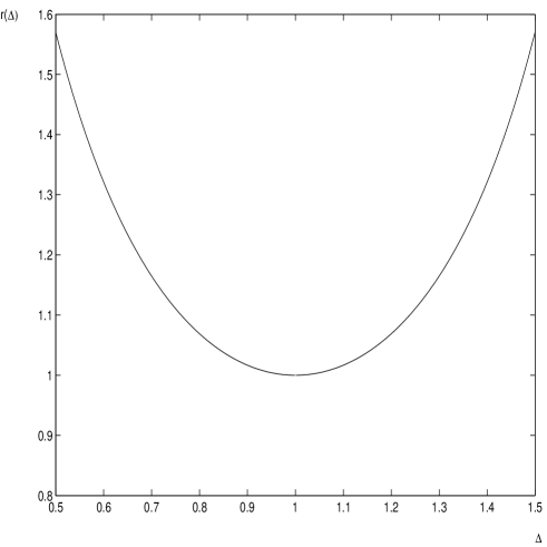
Figure 1: Ratio r between $\|\Delta C^{\pm}_{\infty}\|$ and $\|\Delta C^{\pm}_{1}\|$ versus $\Delta^{\pm}$.

Using the thin lens approximation the $i-th$ contribution to $C_{p}$ can be written

$$(\Delta C_{p})_{i} \simeq A(\theta_{i})\int_{\theta_{i}}^{\theta_{i}+\Delta\theta_{i}}e^{\displaystyle{-i(\Delta-p)\theta}}\mbox{d}\theta=$$ (24)

$$= A(\theta_{i})\frac{i}{|\Delta^{\pm}-p|}e^{\displaystyle{-i(\Delta-p)\theta_{i}}}\left[\cos[(\Delta-p)\Delta\theta_{i}]-1-i\sin[(\Delta-p)\Delta\theta_{i}]\right]\simeq$$

$$\simeq \frac{k_{i}}{\pi(2R)^{N/2}|n_{1}|!|n_{2}|!}\Delta\theta_{i}(\beta_{x})_{i}^{|n_{1}|/2}(\beta_{y})_{i}^{|n_{2}|/2}e^{i[n_{1}(\mu_{x})_{i}+n_{2}(\mu_{y})_{i}-(\Delta-p)\theta_{i}]}.$$

Fig. (1) shows the ratio between $||(\Delta C_{\infty}^{\pm})_{i}||$ and $||(\Delta C_{p}^{\pm})_{i}||$ varying the distance from the resonance ($[\Delta^{\pm}]=1$).
The formulae (13) and (24) give the same result for the modulus of the driving terms when exactly on resonance. A difference between (13) and (24) increases (approximatively) quadratically as one moves away from $\Delta$ integer. Agreement between the two formalism can be therefore expected only if the working point is close enough to the resonance to be compensated .
However, this is not usually the case if the aim is the full compensation of the linear coupling, that is both the sum and difference resonances. In most pratical cases, the working point is close to the difference resonance and relatively distant from the sum resonance.

3.2 Closed-orbit distortion from a dipole kick

The equation (13) can be applied to the resonance family

$${Q_{z}=p}~{}~{}~{}~{}~{}~{}~{}~{}$$ (25)

where $z\equiv x,y$. This leads to the expressions for the closed-orbit distortion due to a dipole kick and links the single resonance theory [6], [16] to the integrated theory of Courant and Snyder [17].
In this case

$$C_{\infty}=\sum_{p=-\infty}^{+\infty}\int_{0}^{2\pi}A(\theta)e^{\displaystyle{-i(Q_{z}-p)\theta}}\mbox{d}\theta$$ (26)

where now [16]

$$A(\theta)=\frac{1}{2^{3/2}\pi R^{1/2}}\sqrt{\beta_{z}(\theta)}e^{\displaystyle{i\mu_{z}(\theta)}}\frac{\Delta B}{B\rho}$$ (27)

($\Delta B/B\rho$ is the dipole error).
For a localized error of length $\Delta l$ (thin lens approximation):

$$(\Delta C_{\infty})_{i} = -\frac{1}{2^{3/2}R^{1/2}}\frac{Q_{z}-[Q_{z}]}{\sin(\pi(Q_{z}-[Q_{z}]))}\sqrt{\beta_{z}}\frac{\Delta l\Delta B}{B\rho}e^{\displaystyle{i(\mu_{z}(\theta)-(Q_{z}-[Q_{z}])\pi)}}=$$ (28)

$$= -\frac{1}{2^{3/2}R^{1/2}}\frac{Q_{z}-[Q_{z}]}{\sin(\pi Q_{z})}\frac{\Delta l\Delta B}{B\rho}\sqrt{\beta_{z}}e^{\displaystyle{i(\mu_{z}(\theta)-Q_{z}\pi)}}.$$

Comparing equation (28) to the closed-orbit distortion (at the origin) due to a kick occurring at a given position $\theta$

$$(z)_{\theta=0}=\frac{\sqrt{\beta_{z}(0)}}{2\sin(\pi Q_{z})}\sqrt{\beta_{z}(\theta)}\frac{\Delta B\Delta l}{B\rho}\cos(\mu_{z}(\theta)-\pi Q_{z})$$ (29)

shows that the normalized orbit distortion differs from $\mbox{Re}(\Delta C_{\infty})_{i}$ by only a constant,

$$\left(\frac{z}{\sqrt{\beta_{z}}}\right)_{\theta=0}\equiv\frac{1}{2^{-1/2}R^{-1/2}(Q_{z}-[Q_{z}])}~{}\mbox{Re}(\Delta C_{\infty})_{i}$$ (30)

3.3 Betatron amplitude modulation

Applying the same procedure to the resonance family

$$Q_{z}=2p.$$ (31)

one gets the modulation of the betatron function due to a small gradient error occurring at a given position $\theta$.
In this case

$$C_{\infty}\equiv=\sum_{p=-\infty}^{+\infty}\int_{0}^{2\pi}A(\theta)e^{\displaystyle{i(2Q_{z}-p)\theta}}\mbox{d}\theta$$ (32)

with

$$A(\theta)=\frac{1}{4\pi R}\beta_{z}(\theta)e^{\displaystyle{2i\mu_{z}(\theta)}}\frac{R^{2}}{B\rho}\frac{\partial B_{y}}{\partial x}.$$ (33)

This gives

$$(\Delta C_{\infty})_{i} = -\frac{1}{2}\frac{Q_{z}-[Q_{z}]}{\sin(2\pi(Q_{z}-[Q_{z}]))}\beta_{z}(\theta)\frac{\Delta l}{B\rho}\frac{\partial B_{y}}{\partial x}e^{\displaystyle{i(2\mu_{z}(\theta)-2(Q_{z}-[Q_{z}])\pi)}}=$$ (34)

$$= -\frac{1}{2}\frac{Q_{z}-[Q_{z}]}{\sin(2\pi Q_{z})}\beta_{z}(\theta)\frac{\Delta l}{B\rho}\frac{\partial B_{y}}{\partial x}e^{\displaystyle{i(2\mu_{z}(\theta)-2Q_{z}\pi)}}.$$

The last expression coincides with the modulation of the beta function (at the origin)

$$\left(\Delta\beta_{z}\right)_{\theta=0}=\frac{\beta_{z}(0)}{\sin(2\pi Q_{z})}\beta_{z}(\theta)\frac{\Delta l}{B\rho}\frac{\partial B_{y}}{\partial x}\cos(2(\mu_{z}(\theta)-Q_{z}\pi))$$ (35)

and shows that the normalized modulation differs from $\mbox{Re}(\Delta C_{\infty})_{i}$ by only a constant,

$$\left(\frac{\Delta\beta_{z}}{\beta_{z}}\right)_{\theta=0}\equiv\frac{1}{(Q_{z}-[Q_{z}])/2}~{}\mbox{Re}(\Delta C_{\infty})_{i}$$ (36)

3.4 Comments

The summed resonance driving terms lead naturally to a new definition of bandwidth. However, pratical differences maybe not so clearly observed. When the working point is close to a resonance, the bandwidth is important but the single and summed theories do not differ much. When the working point is far from the resonance, the bandwidth is unimportant and any widening may go unnoticed.
There is also the more academic point that the magnitude of the summed resonance driving term is dependent on the azimuthal position in the machine. The closed orbit is a very good example of this. If there is a closed bump in the orbit, then the $\mbox{Re}(C_{1,0,\infty})$ is zero outside the bump and finite inside. The implication is that the beam is responding to standing waves from each member of the resonance family. The summed response is the sum of these standing waves. When inside a bandwidth the growth rates are related to the standing wave amplitude and varying according to the position around the machine.

4 The coupled Henon map

In this section, the summed resonance approach is shown to be equivalent to the matrix approach and both are compared to the single-resonance compensation by performing a numerical analysis on the so-called Henon map [8]: a hyper-simplified lattice model whose phase-space trajectories show some of the expected characteristic of a realistic lattice map (nonlinearities, regions of regular and stochastic motion etc.) In this application the linear coupling is generated and corrected by 1+4 thin skew quadrupoles .
The global compensation of the coupling resonances (at $\theta$=0) is achieved if

$$\left\{\begin{array}[]{l}\displaystyle{\sum_{j=1}^{5}[\mbox{Re}(\Delta C^{-}_{\infty})+\mbox{i}\mbox{Im}(\Delta C^{-}_{\infty})]=0}\\ \\ \displaystyle{\sum_{j=1}^{5}[\mbox{Re}(\Delta C^{+}_{\infty})+\mbox{i}\mbox{Im}(\Delta C^{+}_{\infty})]=0}.\end{array}\right.$$ (37)

The compensation for both the sum and the difference resonance is obtained solving the system of 4-equations (for the 4 unknowns $k_{i}$) given by (37).

$k~{}(\mbox{m}^{-2})$	Matrix	Summed	Single
$k_{1}$ (source)	0.5	0.5	0.5
$k_{2}$	-0.051	-0.050	0.559
$k_{3}$	0.034	0.033	0.554
$k_{4}$	-0.319	-0.313	0.476
$k_{5}$	-0.275	-0.275	0.117

Table 1: Compensator strengths ($k_{2-5}$) in presence of the coupling source $k_{1}$ using the single-turn matrix compensation and the summed and single resonance compensations.

Table 1. shows a comparison between the strengths of the 4 correctors ($k_{2-5}$) when compensating the single-turn matrix, the two infinite families of sum and difference resonances (for the same $\theta=0$) and the closest sum and difference resonances to the working point. The single-turn matrix compensation has been performed by means of the MAD program [10] while the (single and multiple) resonance compensation has been obtained making use of the AGILE program [11] in which the formula (13) has been implemented.
The single-turn matrix (in $\theta=0$) in presence of the coupling source $k_{1}=0.5~{}\mbox{m}^{-2}$ (no compensation) has non zero off-axis $2\times 2$ sub-matrices given by

$${\bf T}=\left(\begin{array}[]{cc}M&n\\ \\ m&N\end{array}\right)=\left(\begin{array}[]{cccc}&&0.49&0.49\\ &&0.02&0.02\\ -0.23&-0.24&&\\ -0.01&-0.01&&\end{array}\right)$$ (38)

while the residual values of $n$ and $m$ after the single resonance compensation ($C^{+}=C^{-}=0$) are given by

$${\bf T}=\left(\begin{array}[]{cccc}&&-0.11&-4.67\\ &&0.02&0.15\\ 0.03&-4.57&&\\ 0.03&-0.09&&\end{array}\right).$$ (39)

The off-axis terms are in fact larger after the compensation then before. This is explained by the influence of the far resonances that can not be neglected, to get a satisfactory coupling compensation in this case.
The same conclusion may be drawn by looking at the driving terms of the closest sum and difference resonances before the correction

$$|C^{+}|=0.0628~{}~{}~{}~{}~{}~{}|C^{-}|=0.0628$$ (40)

and afterwards

$$|C^{+}|=0.0207~{}~{}~{}~{}~{}~{}|C^{-}|=0.1018.$$ (41)

Last two equations show that the sets of the uncompensated sum and difference resonances have a ”weight” comparable (larger in the case of the difference resonance) to the ones compensated.

The quantitative difference between the two approaches can be better investigated by means of a tracking analysis.
In the following, the results from stability and footprint diagrams as well as the calculation of the dynamic aperture for the compensated Henon map are shown.

4.1 Stability and footprint diagrams

A stability diagram and the related frequency diagram can be obtained by the following procedure: for each initial condition inside a given grid in the physical plane $(x,y)$ ($p_{x}=p_{y}=0$), the symplectic map representing the lattice is iterated over a certain number of turns. If the orbit is still stable after the last turn, the nonlinear tunes can be calculated using one of the methods described in [12]. In the stability diagram the stable initial conditions are plotted whereas in the frequency diagram are represented the corresponding tunes. The insertion in the frequency (footprint) diagram of the straight lines representing the resonant conditions up to a certain order makes it possible to visualize the excited resonances close to the reference orbit.

Figs. (5) - (10) show the stability and frequency diagrams for the uncoupled Henon map, after the single resonance compensation and after the summed resonance one.
The comparison points out that the summed resonance compensation allows a more efficient restoration of the uncoupled optics. It is significant the analysis of the degree of excitation relative to the resonances (3,-6), (1,-4) and (2,-5) for the two different compensation approaches.

Using the perturbative tools of normal forms [13] one can calculate the value of the first resonant coefficient (leading term) in the interpolating Hamiltonian for the considered resonances. The leading term can be considered as a ”measure” of the resonance excitation. It can be shown [14] that in absence of coupling the leading term of the resonances (3,-6) and (1,-4) is different from zero (first order excitation) whereas the one of the resonance (2,-5) is zero (second order excitation). The strength of the coupling (that is, in the considered case, the strength of the residual coupling after the compensations) is proportional to the growth of the leading term of the first order non-excited resonances and to the decrease of the leading term of the other ones.
The resonance degree of the excitation varying the compensation approach can be better visualized ploting the network of the resonances and their widths inside the stability domain. The analysis of Figs. (2)-(4) confirms that the SR method is characterized by a residual coupling considerably stronger than the one left by the MR compensation.
The same conclusion can be drawn the following topological argument. A trace of the presence of linear coupling in a nonlinear lattice is the spliting of the resonant channels in correspondence of the crossing points (multiple resonance condition in the tune space). This phenomenon is evident only in the case of the MR compensation (see the central part of Fig. (4)).

Figure 2: Network of resonances of the uncoupled Henon map.

Figure 3: Network of resonances after the summed resonance compensation.

Figure 4: Network of resonances after SR compensation.

4.2 Dynamic aperture calculations

The dynamic aperture as a function of the number of turns $N$ can be defined [15] as the first amplitude where particle loss occurs, averaged over the phase space. Particle are started along a grid in the physical plane $(x,y)$:

$$x=r\cos\theta~{}~{}~{}~{}~{}~{}~{}~{}~{}~{}~{}~{}~{}y=r\sin\theta$$ (42)

and initial momenta $p_{x}$ and $p_{y}$ are set to zero.
Let $r(\theta,N)$ be the last stable initial condition along $\theta$ before the first loss (at a turn number lower than $N$). The dynamic aperture is defined as

$$D=\left[\int_{0}^{\frac{\pi}{2}}[r(\theta,N)]^{4}\sin(2\theta)\mbox{d}\theta\right]^{\frac{1}{4}}.$$ (43)

An approximated formula for the error associated to the discretization both over the radial and the angular coordinate can be obtained replacing the dynamic aperture definition with a simple average over $\theta$. Using a Gaussian sum in quadrature the associated error reads

$$\Delta D=\sqrt{\frac{(\Delta r)^{2}}{4}+\left\langle\left|\frac{\partial r}{\partial\theta}\right|\right\rangle^{2}\frac{(\Delta\theta)^{2}}{4}}$$ (44)

where $\Delta r$ and $\Delta\theta$ are the step sizes in $r$ and $\theta$ respectively.
In Tab. 2 the values (with the associated errors) of the dynamic aperture are quoted for the three studied optics for short ($N$=5000) and medium ($N$=20000) term tracking.

$D$ (m)	Uncoupled	Summed	Single
$N$=5000	0.0406	0.0412	0.0372
$N$=20000	0.0405	0.041	0.037

Table 2: Dynamic aperture values relative to the uncoupled Henon map and after the summed and single resonance compensations. The associated error (according to the formula (44)) is about 2% for $N$=5000 and about 4% for $N$=20000.

The difference between the summed and the single resonance compensations is noticeable: the compensation of the all families relative to the coupling resonances allows an improvement close to 10% respect to the case in which the high frequency part of the perturbative hamiltonian is neglected.
It can also be pointed out that the summed compensation seems to slightly improve (at the limit of sensitivity due to errors) the dynamic aperture respect to the uncoupled case.

5 The nonlinear case

Dealing with high-order resonances with a view to optimizating stability is not so straightforward as in the linear case: the number of resonances that can be excited both by a given multipole and by the set of correctors meant for compensating a given resonance becomes higer and higher; moreover the resonance compensation is only one of the tools that has to be used to get a succesfully optics optimization.

For these reasons we have not here attempted a general comparison between the summed and the single resonance compensations using tracking analysis. We intend to return to this question in the future.
We note however that a certain number of attempts to compensate one particular sextupolar resonance for the Henon map show that the two compensations are not far only if the working point is close enough to the considered resonance. The summed resonance compensation is to in general better in the case of the compensation of several resonances at the same time.

6 Conclusions

A general method has been derived for the summation of all the resonances within a given family both for the linear and for the non-linear cases. The fact that this summation is valid and gives a meaningful result is confirmed by its application to the known closed-orbit distortion equation, the betatron modulation equation and the decoupling of the linear transfer matrix for a ring. The application of the summed-resonance driving term to the coupling raises the question of the relative merits of the different types of coupling compensation that are now possible. This problem has been investigated with the help of the Henon map. The results indicate that use of the summed-resonance compensation (equivalent to the matrix approach) yields a larger dynamics aperture.

Acknowledgements

The work of D. Fanelli is supported by a Swedish Natural Science Research Council graduate student fellowship. We thank P.J. Bryant and E. Aurell for discussions and critical reading of the manuscript.

Figures caption:

$~{}~{}~{}\bullet$  Figure 5: Stability domain of the uncoupled Henon map.

$~{}~{}~{}\bullet$  Figure 6: Footprint diagram of the uncoupled Henon map.

$~{}~{}~{}\bullet$  Figure 7: Stability domain after the summed resonance compensation.

$~{}~{}~{}\bullet$  Figure 8: Footprint diagram after the summed resonance compensation.

$~{}~{}~{}\bullet$  Figure 9: Stability domain after the single resonance compensation.

$~{}~{}~{}\bullet$  Figure 10: Footprint diagram after the single resonance compensation.

References

- [1] P. J. Bryant, K. Jonshen, The principles of Circular Accelerators and Storage Rings, Cambridge University Press (1993)
- [2] D.C. Carey, The optics of charged particles beams, Harwood Academic Publishers (1987)
- [3] D. Edwards, L. Teng, Parametrization of the linear coupled motion in periodic systems, IEEE Trans. Nucl. Sci. (1973).
- [4] R.Talman, Coupled betatron motion and its compensation,US-CERN School of Particle Accelerators, Capri, Italy (1988).
- [5] S. Peggs, Coupling and decoupling in storage rings, PAC 1983.
- [6] G. Guignard, J. Hagel, Hamiltonian treatment of betatron coupling, CERN 92-01 (1992).
- [7] P.J. Bryant, A simple theory for weak betatron coupling, CERN 94-01 (1994).
- [8] M. Henon, Numerical study of quadratic area preserving mappings, Appl. Math. 27 (1969) 291-312.
- [9] I.S. Gradshteyn, I.M. Ryzhik, Table of Integrals, Series and Products, Academic Press, London (1980).
- [10] H. Grote, F.C. Iseline, The MAD program, User’s Reference Manual, CERN/SL/90-13 (1990).
- [11] P.J. Bryant, AGILE-lattice program, in preparation.
- [12] R. Bartolini, M. Giovannozzi, W. Scandale, A. Bazzani, E. Todesco, Algorithms for a precise determination of betatron tune, Proc. of EPAC 96, Sitges, vol. II, pag. 1329 (1996).
- [13] A. Bazzani, G. Servizi, E. Todesco, G. Turchetti,A normal form approach to the teory of nonlinear betatronic motion, CERN Yellow Report (1994).
- [14] G. De Ninno, E. Todesco, Effect of the linear coupling on nonlinear resonances in betatron motion, Phys. Rev. E, 2059-2062 (1997).
- [15] E. Todesco, M. Giovannozzi, Phys. Rev. E 53, 4067 (1996).
- [16] G. Guignard, The general theory of all sum and difference resonances in a three-dimensional magnetic field in a synchrotron, CERN 76-06 (1976).
- [17] E.D. Courant, H.S. Snyder, Theory of the Alternating-Gradient Synchrotron, Annals of Physics 3, 1 (1958).