A possible explanation for Earth’s climatic changes in the past few million years

Abstract

The astronomical theory of Milankovitch relates the changes of Earth’s past climate to variations in insolation caused by oscillations of the orbital parameters. However, this theory has problems to account for some major observed phenomena of the past few million years. Here, we present an alternative explanation for these phenomena. It is based on the idea that the solar system until quite recently contained an additional massive object of planetary size. This object, called Z, is assumed to have moved on a highly eccentric orbit bound to the sun. It influenced Earth’s climate through a gas cloud of evaporated material. Calculations show that more than once during the last 3.2 Myr it even approached the Earth close enough to provoke a significant shift of the geographic position of the poles. The last of these shifts terminated the Earth’s Ice Age epoch. The origin and fate of Z is also discussed.

1 The problem of Earth’s past climate changes

Ancient climate is recorded in deep sea sediments, polar ice and some other natural archives mainly through changes in the oxygen isotope ratio, the $\delta^{18}$O. In deep sea sediments the $\delta^{18}$O-signal reflects the combined effect of water temperature and of the amount of ice on Earth, whereas in polar ice it is a reliable proxy for the ambient local surface air temperature at the time of freezing. The study of paleontology and isotopic composition of hundreds of drilling cores extracted from these archives during the last few decades confirm that Earth’s past climate changed between colder and warmer phases, known as the glacial-interglacial cycles. Spectral analysis of this kind of proxy data covering the Late Pleistocene have yielded periodicities, which agree more or less with those of Earth’s main orbital parameters, i.e. precession (23 kyr), obliquity (41 kyr) and eccentricity (100 kyr), which appear at first sight to support the old idea of Milankovich [1], that Earth’s climate reflects the variation in insolation (solar heating) caused by the combined effect of the variation of these parameters [2, 3]. However, this astronomical theory of climate has several shortcomings. In particular, the main glacial-interglacial transitions occurred approximately every 100 kyr. This feature contradicts the astronomical calculations which show that the modulation of the insolation due to the eccentricity oscillation is negligibly small compared to that of the two other orbital parameters. Many hypotheses have been formulated to explain this “100 kyr problem”, sometimes involving additional astronomical parameters, such as the oscillation of the inclination of Earth’s orbital plane, whose periodicity equals that of the eccentricity [4, 5]. Most of the more recent attempts to understand this problem rely either on a non-linear response of the ice-sheet dynamics [6], or of that of the coupled Atmosphere-Ocean system to the astronomical insolation forcing [7]. Although the results of some of these models compare well with the time spectra of the climate record, up to now none of them could reproduce the amplitude and phase of each glacial cycle. For instance, one of the most prominent interglacial periods of warmings observed around 400 kyr ago, known as the “isotope stage 11”- problem, happened at the time when the solar insolation was smaller than during the glacial times prior to and after this period. More recent measurements with improved time resolutions, on deep sea sediment [8, 9] and polar ice cores, GRIP [10], GISP2 [11] and Vostok [12] revealed some additional and most puzzling features of past climate. Fig. 1 shows the well known $\delta^{18}$O-record of the GRIP ice core covering the last 130 kyr of Earth’s climate history, including the last interstadial, the Eem, the last glacial maximum around about 18–20 kyr BP, and its abrupt termination at about 11.5 kyr ago. Although some discrepancies between the GRIP and GISP2 data older than about 100 kyr BP have been noted [11], it is evident, that Earth’s climate changed rapidly during the last Ice Age period. These temperature peaks, called Dansgaard-Oeschger events, cannot be explained in terms of the Milankovitch effects, since they are too fast in comparison with the orbital parameters induced solar insolation variations. Even more puzzling is the fast termination of the last Ice Age period, the Pleistocene-Holocene transition, shown in the lower part of Fig. 1. This transition ended the Pleistocene, and the following Holocene is a period of warmer temperature and generally more stable climate. It has been demonstrated that the climatic system in the Northern hemisphere is capable to switch rapidly from one given state to another [13]. But again, if for the same reason as mentioned above the Milankovitch effect cannot be the cause of such a switch, what else could it be? Is it possible that the luminosity of the sun varied in accordance with these observations? This is very unlikely, because prior to the Ice Age epoch, i.e. during the Late Pliocene until about 3.3 Myr ago, the climate was mild, stable for millions of years, and very similar to what it has been since the beginning of the Holocene [9]. Why should the irradiance of the sun suddenly get noisier for a limited time? The Milankovitch effect and small changes of the solar irradiance are of relevance for Earth’s climate. However, we agree with some of the critics pointing out that both possibilities fail to explain many properties of the observed past changes of climate and that new ideas are required to solve the riddle of the Ice Age [4, 6].

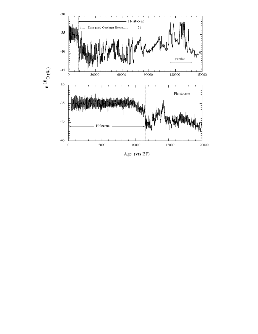
Figure 1: Upper part: Ice core $\delta^{18}$O record (GRIP) over 150 kyr [10]. This time span covers the last Interstadial, the Eemian, the last glacial period (ca. 90 – 11.5 kyrs) which is characterized by transient and fast temperature variations (21 Dansgaard-Oeschger events), and the Holocene reflecting the sudden improvement of Earth’s climate at about 11.5 kyrs ago. The lower part is an expanded view of the same record for the last 20 kyrs. It shows the time structure of the Dansgaard-Oeschger event No.1 and the fast Pleistocence-Holocene transition as indicated by the vertical dashed line.

In what follows we present such a new idea. First, we show that the fast termination of the last Ice Age period, the Pleistocene-Holocene transition, can best be understood in terms of a rapid polar wandering, as has been suggested (and refused) more than 100 years ago. We then demonstrate that such a shift can occur during a close encounter between an object of planetary size and the Earth. Assuming that this object, called Z, was on a highly eccentric orbit bound to the sun, we find that it could be responsible for Earth’s climatic changes over the last few million years. Z must have disappeared from the solar system some time after the polar shift event, and we also consider the mechanisms responsible for its disappearance.

2 Evidences for a polar shift event at the end of the last Ice Age period

The Last Glacial Maximum (LGM) around 18–20 kyr BP is characterized by the lowest known temperature in Earth’s history, low precipitation rates, reduced sea level of at least 120 Meter [14], and huge polar ice shields extending over the northern part of America down to a latitude of almost 40^∘ N during the last glacial maximum (Wisconsin stage), and in Europe to about 50^∘ N, known as Weichsel and Würm stages in its northern part and in the Alps, respectively [15]. It is also well documented that at the same time large flocks of Mammoths, Woolly Rhinos and many other species of mammals roamed in north-eastern Siberia and north-western Alaska [16]. Remains of these animals have been found on the New Siberian Islands as far as 76^∘ North indicating that food was available to support these largest mammals throughout the Late Pleistocene. It has also been noted, that at the same time this part of the world was covered by non-arctic forests up to about the same latitude, e.g. more than 1000 km within present days’ arctic cycle (66,66^∘). Even more puzzling, however, is the evidence that at the end of the last ice age, the so called Pleistocene-Holocene transition, these animals were not only instantaneously killed by some yet unknown cause, but also immediately deep frozen together with the surrounding mud [17]. The fact that the flesh of some of these animals was still eatable (for dogs) at the time of their discovery about 200 years ago suggests temperatures below freezing point throughout the Holocene in this part of the world. This is in contrast to the general warming up observed in many other places on Earth including both polar regions. The observation of simultaneous mass extinctions of small and large animals in the western part of Alaska, in Western Europe and North America [18, 19] and the distinct sea level rise leave no doubt that the observed fast rise in temperature at the end of the last ice age period was accompanied by a global cataclysm and a rapid reorganization of the global climate.

During the LGM the northern polar ice cap was not centered at the position of the (present day) north pole, but displaced by about 18–20 degree southwards on the American side of the globe [15]. This introduced the possibility of a rapid polar wandering, i.e. a change in orientation of the Earth with respect to its rotation axis. This idea was considered in detail more than 100 years ago by the most eminent scientists of that time such as G.H. Darwin, J.C. Maxwell, G.V. Schiaparelli, W. Thomson and many others. They concluded that such a turn of the globe changing the geographical position of the North Pole to the amount required by the observations is in principle possible, but would require a force sufficient to overcome the stabilizing effect of the equatorial bulge of our planet, which acts like the rim of a gyroscope. Since they were unable to find any terrestrial or extraterrestrial mechanism that could give rise to such a force, this idea was finally dismissed as impossible and, in fact, “not worth discussing” [20]. Only more recently was this verdict seriously questioned when the evidence from rock magnetism studies unmistakably suggested that the wandering of the geographic poles was more rule than exception in Earth’s history [21, 22]. However, this wandering is a slow process, probably connected to the continental drifts first predicted by Wegener [23], and therefore it cannot explain the rapid termination of the last ice age. In view of this dilemma, Hapgood [20] suggested an alternative possibility based on the idea that the observed changes reflect the occasional sliding of the whole rigid crust over the viscous, plastic or possibly fluid inner layers of our Earth. He showed that the mass of the Antarctic ice cap is not symmetrically distributed about the rotation axis and believed that the resulting centrifugal effect is sufficiently large to initiate such a slippage, provided the ice cap can re-grow large enough after each slide. In his foreword to Hapgood’s book, A. Einstein cautiously commented this idea as follows: “The only doubtful assumption is that the Earth’s crust can be moved easily enough over the inner layers”. This is indeed the crucial point of this idea which eventually has not been accepted.

Was this the end of the polar shift debate, although a fast polar shift is still the most straightforward explanation for all observed effects connected with the fast termination of the last Ice Age period? In further investigating this question, we found that one particular excitation mechanism, namely the deformation of the Earth in a transient external gravitational field gradient, can produce the required effect.

3 The excitation of a polar shift during a close flyby of a massive object

Any redistribution of Earth’s mass is accompanied by a wobble and turn of the entire Earth relative to its rotation axis. This movement depends on both the initial mass redistribution and the rate at which the Earth’s rotational bulge can readjust to the changing position of the rotation axis on the globe. Generally, the polar wandering resulting from Earth-bound causes are either too slow (drift of the continental plates), or too small (storm, ocean currents), to produce the rapid and large shift required to explain the fast termination of the last ice age period. But what about cosmic events? There are two possibilities worthwhile to be considered: A collision of an object with the Earth, and a close flyby of an object. The first case has previously been discussed in the Literature [24]. It can be dismissed, because an impact, capable to significantly alter Earth’s angular momentum or its moment of inertia, would have left one or several craters and other distinct geophysical and chemical signatures, which would have been discovered by geologists, bearing in mind that the event we are discussing occurred only 11.5 kyr ago. We therefore consider the possibility that the Earth had a close encounter with a massive object. We estimate first the minimum amount of deformation required to cause a polar wandering of about 18^∘, as is mentioned in chapter 2. We then show that such a shift can be induced by an object of planetary size during a flyby and that it is fast enough to explain the rapid termination of the last Ice Age epoch.

3.1 Earth’s deformation in a strong gravitational field gradient

Prior to any disturbance the rotating Earth is to a large extent in a hydrostatic equilibrium. The moment of inertia is a symmetric tensor $\Xi$ which connects the vectors of angular velocity $\vec{\omega}$ and angular momentum $\vec{D}$ by the equation $\vec{D}=\Xi\vec{\omega}$. For the undisturbed Earth the diagonalized tensor has the elements $\Xi[1,1]\equiv A=\Xi[2,2]\equiv B=8.010247\cdot 10^{37}$ kg m² and $\Xi[3,3]\equiv C=8.036559\cdot 10^{37}$ kg m² [25]. The ratio $C/A=1.0032847$ shows that the equatorial bulge contributes about 3.3 %₀ to the main principal moment of inertia; the radius at the equator exceeds that at the poles by about 21 km. This equatorial bulge stabilizes the position of the rotation axis along the figure axis C. During the flyby of a massive object, the globe is transiently deformed so that the new principal axis of the inertial tensor $\Xi$ — the figure axis — deviates from the rotation axis. These axes then precess around each other, whereby the angular momentum $\vec{D}$ remains fixed in space. For an observer on Earth the angular velocity vector $\vec{\omega}$ moves around the figure axis. In co-ordinates fixed to the Earth this free motion is described by the Euler equation

$$\frac{d\Xi\,\vec{\omega}}{dt}=[\Xi\,\vec{\omega},\vec{\omega}]$$ (1)

where the square bracket represents the vector product. According to Eq. 1 the precession frequency of a rigid Earth would be $\omega_{0}(C-A)/A$, with $\omega_{0}$, the angular velocity of Earth’s rotation. This yields an “Euler period” of 305 d. A minute precession of the rotation axis was observed by S.C. Chandler more than 100 years ago, but its period turned out to be 435 d [26]. Newcomb [27] showed that this discrepancy can be understood by assuming that the Earth is not rigid but can be plastically deformed, which was quite a pioneering conclusion in those days. Since then, this so called Chandler’s free motion of the rotation axis has been studied in great detail, but always in view of small deviations only [28, 29]. The presently continuing Chandler motion is still open to discussion [30].

A massive object passing the Earth at a close distance deforms it with a time dependent tidal force, which is the difference between the gravitational force at the given point and that acting at the Earth’s center. When the distance $R$ between the centers of the two masses is large compared to the radius $R_{E}$ of the Earth, the tidal force $\vec{F}(z)$ is parallel to the z-direction which points to the perturbing mass $M_{Z}$. It has the value

$$F(z)=2M_{Z}Gz/R^{3}$$ (2)

where $G=6.673\cdot 10^{-11}$ m³kg^-1s^-2 is the gravitational constant. On Earth’s surface $z=R_{E}\cos\gamma$, where the angle $\gamma$ is the latitude. This tidal force increases as the third reciprocal power of the distance $R$ between the center of the perturbing mass and that of the Earth. For example, if the moon would be 10 times closer to the Earth, then its tidal force would be 1000 times larger than it is at present.

In first order approximation, this force tends to give the Earth an ellipsoidal shape. Such a deformation is possible because Earth’s interior is liquid or plastic except for the inner core and the peripheral crust [25]. We estimate the deformation due to the force, Eq. 2, in a static approach by minimizing the energy as a function of the deformation in the external field. For this we assume that the redistribution of material at the surface of the Earth is given by

$$H(\gamma)=H_{0}(\cos(2\gamma)+1/3)$$ (3)

where $H_{0}$ is the amplitude of the tide. The energy of the material in the deformed state minus that prior to the deformation in the presence of the perturbation is then

$$\Delta E(H_{0})=\frac{32\pi}{45}\rho R_{E}^{2}\left(H_{0}^{2}g-\frac{H_{0}M_{Z}GR_{E}^{2}}{R^{3}}\right)$$ (4)

which is minimized with

$$H_{0}=R_{E}^{2}M_{Z}G/(2R^{3}g)$$ (5)

Here $g$ = 9.8 m/s² is the gravitational acceleration at the surface of the Earth and $\rho$ the specific weight of the displaced material (3500 kg/m³ for the Earth’s surface). Applying Eq. 5 to the Earth-Moon system we find that the peak-to-peak level difference on Earth induced by our Moon is $2H_{0}$ = 0.35 m which agrees quite well with the recently evaluated deformation of about 0.30 m [31]. We use this formula to estimate the deformation produced by a flyby of a massive object, although we are aware that this simple approach probably overestimates the deformation remaining immediately after such a flyby. In particular, if the response to the strong tidal force is too fast, then part of the deformation will quickly disappear when the force ceases. We also expect that the actual deformation will not be a linear function of the gravitational force, and will depend on the relative motion of the perturbing mass to the surface of the rotating Earth.

To estimate the minimum amplitude $H_{0}$ of the tidal bulge required to cause a polar wandering of about 18^∘, as explained in chapter 2, we added to the equilibrium deformation of the Earth an additional mass distribution of the form of Eq. 3, which was rotated by an angle $\alpha$ with respect to the original figure axis. The diagonalization of the new inertial tensors resulted in a new figure axis whose tilting angle relative to the former axis depends on $H_{0}$ and $\alpha$. Minimizing $H_{0}$ as a function of $\alpha$, we find that a tilting angle of 18^∘ can be achieved with a bulge amplitude of $H_{0}$ = 6.45 km and an angle $\alpha$ = 30^∘. This result allows us to estimate the mass of our flyby-object or its distance of closest approach, by means of Eq. 5 which fixes $M_{Z}/R^{3}$. Assuming for instance that the distance of closest approach should be larger than the Roche limit, which for our Earth is about $R_{l}=2.44R_{E}$, i.e. 15’600 km (assuming equal density of both objects), then the mass $M_{Z}$ must be larger than about 0.03 times the mass of the Earth ($M_{E}$), a value which is somewhat smaller than that of Mercury. On the other hand, 2-body dynamics tells us that the mass has to be much smaller than that of our Earth. Otherwise Earth’s orbit, in particular its inclination and eccentricity, would have been altered during such an event to an amount which would be incompatible with the present orbital parameters of the Earth. This consideration suggests an upper limit of about $M_{Z}<0.2M_{E}$, and, according to Eq. 5, a maximum distance of closest approach of 29 300 km. Since our static approximation most probably overestimates the tidal effects, we suspect that the mass of Z was larger than 0.03 $M_{E}$ and that its closest approach during this event was even within the Roche limit.

3.2 The fast polar wandering

The sudden deformation of the Earth resulting from a short flyby event (the excitation time is less than 10 h) defines the new figure axis around which the rotation axis immediately starts to precess, as described by Euler’s Eq. 1. Since the figure axis itself moves only by small amounts in co-ordinates fixed to the Earth, the rotation axis effectively spirals to the shifted position of the figure axis. To demonstrate this polar wandering, we solved Eq. 1 numerically. Since the Earth is not a rigid body we started the calculation with the inertial tensor, as defined by the initial deformation, and assumed that it relaxes towards the equilibrium tensor $\Xi_{0}$ oriented along the instantaneous rotation axis as

$$\frac{d\Xi}{dt}=-\frac{\Xi(t)-\Xi_{0}[\vec{\omega}(t)]}{\tau}$$ (6)

Thus we approximated the relaxation behavior by a single relaxation time $\tau$, which includes both the capability of the equatorial bulge to follow the rotation axis and the disappearance of the deformation responsible for the polar wandering. Assuming a relaxation time of $\tau$ = 500 d, we find that the rotation axis moves into the new position with a precession period of about 400 d. The final destination is reached within about four precession periods or about 4.8 years (Fig. 2).

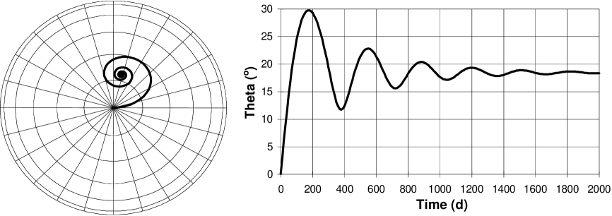
Figure 2: Left side: Geographic movement of the rotation axis induced by the flyby of a massive object, assuming the deformation and relaxation parameters discussed in 3.1. and 3.2. The circles are latitudes with respect to the previous pole position, spaced 15^∘. Right side: Time dependence of the angle $\Theta$ between the angular momentum (fixed in space) and the previous pole direction.

This is certainly fast enough to explain the rapid termination of the last Ice Age period shown in the lower part of Fig. 1. We have to add here, that the true relaxation behavior of the Earth in the presence of a large, but short-term deformation is still open to speculation. The theoretical estimates for this relaxation time vary between a few 10 d and 10 yr [32]. We find that $\tau$ in our example has to be larger than about 100 days to achieve a polar shift of the required magnitude.

3.3 The impact of the polar shift event on the climate

The lower part of Fig. 1 shows, that the termination of the last ice age period is characterized by two events: A short term increase of temperature around about 14.5 kyr. ago, which was followed by a slow decrease back to the Ice Age level. The following cold period, known as Younger Dryas (YD), lasted for about 800 years. At about 11.5 kyr ago the temperature suddenly rose again, but, and in contrast to the previous event, it continued to increase slowly until about 9000 years ago. From then on the surface temperature over Greenland essentially remained at that high value up to the present day. Can we understand why the first temperature increase was a transient episode only, whereas the second event had such a long lasting effect? To answer the first part of this question we need to consider an additional property of our flyby object, which will be discussed in the next chapter. It is sufficient to mention here that in this case the flyby distance of our object was simply too large to excite a significant polar wandering. The consequences of the second event can be explained in terms of the polar wandering discussed above. For this we have to remember (see chapter 2) that the shape and extension of the ice shield in the Northern hemisphere prior to the shift suggest a pole position at a longitude of about 90^∘ W and a latitude of about 72^∘ N, which is quite close to the present position of the North magnetic pole. Identifying this position with the starting point of our calculation presented in Fig. 2, we see that the net effect of this polar wandering was a rotation of the globe by about 18^∘. As a consequence, the latitudinal pattern of the incident solar radiation immediately changed, so that, e.g. the low latitude part of the North American and European ice shields rapidly melted away, whereas in formerly ice free regions of the Arctic Ocean permanent ice was formed. Similarly, in the eastern part of the Antarctic the extent of the ice shelf was reduced, and, as we suspect, the formerly ice free western coast was covered to the extend observed today. After a transition time of about 2 000 years during which the polar ice sheets adjusted to the new pole position, the new state of the climate, called Holocene, was established. Compared to the previous climate state, the Holocene is significantly warmer, essentially, because the North pole moved away from the upper part of the North American continent into the present position in the Arctic Ocean. This resulted in an increased heat exchange between ice and water, which significantly reduced the extent of the polar ice cap. The albedo decreased accordingly. This reduction was only partially compensated by the corresponding changes in the southern hemisphere. According to this scenario, the Holocene is a new stable epoch and not just another Interstadial, as is generally believed, because the new pole position is stable and Z no longer influences the Earth.

4 Planet Z: a transient member of the solar system

We have seen that an object of mass $M_{Z}$ between 0.03 $M_{E}$ and 0.2 $M_{E}$ can excite a polar shift which is both fast and large enough to explain the termination of the last Ice Age, provided it passed the Earth at a distance of less than about 30 000 km. Since it is extremely unlikely that an object on a hyperbolic trajectory would accidentally approach the Earth so close during one singular flyby, we consider the possibility that it was moving on a bound orbit extending beyond that of the Earth. The problem with this assumption is that this object, Z, no longer exists — otherwise we would observe it — so that the occurrence of the proposed close encounter at a specific time cannot be verified by backward calculations. Therefore, we shall consider the long term behaviour of Z on the basis of assumed orbital parameters in order to find out whether close approaches to the Earth occur as often as expected. We shall see that this “trial and error” approach not only gives a positive answer, but even provides an explanation for the frequent fast climatic changes observed prior to the pole shift event (see chapter 5).

4.1 The orbit of planet Z and its close encounters with the Earth

There are constraints on the initial orbital parameters of Z. Its aphelion has to be larger than that of the Earth, otherwise it could not approach the Earth close enough. We shall see further below that at each perihelion passage a surface layer of Z has to evaporate at sufficiently high temperatures so that atoms reach the escape velocity. This requires an extremely eccentric orbit with $a\ll b$, where $a$ is the perihelion and $b$ the aphelion distance. Thus the major semi-axis $A=\frac{1}{2}(a+b)\approx\frac{1}{2}b$ must be larger than 0.5 AU, and the eccentricity $\epsilon=(1-a/A)$ close to one. Expecting that the encounter frequency rapidly decreases with increasing $A$, we restrict the investigations, to the range $0.5<A<2$ AU. There are no restrictions on the inclination $i$ of Z’s orbit, so that the full range $0^{\circ}<i<180^{\circ}$ has to be explored.

With this in mind, Nufer et al. [33] calculated the movement of Z in the gravitational field of the sun, the Earth, the Moon and all other planets, except Uranus, Neptune and Pluto, and evaluated by means of a Pascal program its closest approaches to the Earth for each orbital period. Details of this program, its performance, and the relevant results shall be published in [33]. In the simulations Z was always added to the solar system at the year J2000.0, ignoring the fact that at this time it no longer existed. So far calculations have been performed, forward as well as backwards in time, for two different masses ($M_{Z}=0.11M_{E}$ equal to that of Mars, and $M_{Z}=0.06M_{E}$) and seven different sets of initial orbital parameters ($A=0.978$ and 2 AU, six different inclinations in the range $i=0^{\circ}$–$180^{\circ}$ and two eccentricities $\epsilon=0,973$ and 0.987) The time ranges varied between 150 and 750 kyr. As expected, we found that encounters are more frequent for $A=0.978$ than for $A=2$. Their number also increases with increasing eccentricity $\epsilon$, and is largest for small inclinations $i<6^{\circ}$. The inclination is defined here as the angle between Z’s orbital plane and the invariable plane which is perpendicular to the orbital angular momentum of the solar system. The results obtained with the initial conditions $A=0.978$, $\epsilon=0.973$, $i=0^{\circ}$ and $180^{\circ}$, respectively, are too similar to decide whether Z was on a pro- or a retrograde orbit. Since the computing speed strongly depends on the precision assumed for the numerical integration procedure, we restricted it to a moderate value of $10^{-13}$ per integration step, which was sufficient for most considerations. With this restriction, about 15 h were needed to cover 10 kyr using a 133 MHz PC.

The result of one of these calculations is displayed in Fig. 3.

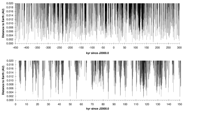
Figure 3: Upper panel: Closest approaches of planet Z ($M_{Z}=0.11M_{E}$) to the Earth over 750 kyr and to distances of less than 0.02 AU = $3\cdot 10^{6}$ km as indicated by the endpoint of each vertical line. Lower panel: Expanded view of the irregular clustering of these approaches over 150 kyr.

It shows the closest approaches of Z ($M_{Z}=0.11M_{E}$) to the Earth over a time period of 750 kyr. The initial parameters at J2000.0 were $A=0.978$ AU, $\epsilon=0.973$ and $i=0^{\circ}$. Plotted are all encounters with distances of less than 0.02 AU = $3\cdot 10^{6}$ km. The irregular clustering of these approaches is the result of the osculating orbital parameters of Z and the Earth. An expanded view of all closest approaches with distances less than twice that of the Moon over 750 kyr is given in Fig. 4.

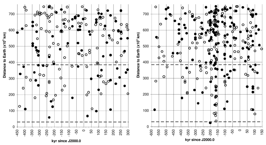
Figure 4: Closest approaches over 750 kyr below twice the Moon-Earth distance. The pattern depends on the selected orbital parameters and the mass of the object. The left side shows the result obtained for a mars-like object ($M_{Z}=0.11M_{E}$), and the right side that for an object with $M_{Z}=0.06M_{E}$ but otherwise identical start parameters. The two horizontal dashed lines in both figures indicate Moon’s distance (384 000 km), and the critical distance below which significant polar shifts have to be expected (30 000 km), respectively. The open (filled) circles mark the encounters of the objects on their way towards (from) the sun.

To illustrate the mass dependence we also show the pattern obtained for an object with $M_{Z}=0.06M_{E}$, but otherwise identical orbital parameters. The two horizontal dashed lines in both figures indicate Moon’s distance (384 000 km), and the critical distance below which significant polar shift events have to be expected (30 000 km). In the first case we note a closest approach of about 59 000 km, i.e. no pole shift event, but a distinct one in the second case (23 500 km). From these and the other trials we conclude that an object moving on a highly eccentric orbit approaches the Earth to polar shift distance about once in 1 Million years, which is compatible with the duration of the ice age epoch (see chapter 6.1). It is meaningless that the calculated polar shift event does not occur at the expected time in view of the fact that the exact mass and orbit of Z is unknown. In both cases we also observe about 6 flyby’s per 100 kyr below 300 000 km. In all these events the gravitational interaction is still strong enough to excite strong earthquakes and volcanic activities (see chapter 7). All these close flyby’s also influence Moon’s orbit. We found, however, that the resulting disturbances over the investigated time ranges are averaged to the amount compatible with the present orbit [33]. The frequency of the flyby’s increases with their distance. For distances larger than twice that of the Moon they are harmless regarding tidal effects induced on Earth, but they can still influence Earth’s climate. To understand this additional effect, which is further discussed in chapter 5, we next examine what happened to Z on the proposed highly eccentric orbit. For convenience, we assume that it was a Mars sized object with $M_{Z}=0.11M_{E}=6.58\cdot 10^{23}$ kg, and radius $R_{Z}=3.39\cdot 10^{6}$ m.

4.2 Solar radiation effects: the gas cloud

An object moving on a highly eccentric orbit is exposed to intense solar radiation. The total amount of energy $E_{Zs}$ received by Z per unit of surface and orbital period is

$$E_{Zs}=P_{s}\oint\frac{dt}{4\pi R^{2}}=\frac{M_{Z}}{2L}P_{s}$$ (7)

where $P_{s}=3.73\cdot 10^{26}$ J/s is the total power radiated by the sun. The orbital angular momentum $L=M_{Z}R^{2}\frac{d\varphi}{dt}\quad(M_{Z}$: mass of Z, $R$ its distance to the sun, and $\varphi$ the angle co-ordinate) is determined by the major semi-axis $A$ and the eccentricity $\epsilon$

$$L=M_{Z}\sqrt{M_{S}GA(1-\epsilon^{2})}$$ (8)

$G$ is the gravitation constant, and $M_{S}$ the mass of the sun. Therefore

$$E_{Zs}=\frac{1}{2}\frac{P_{s}}{\sqrt{M_{S}GA(1-\epsilon^{2})}}$$ (9)

Using the same orbital parameters as in Fig. 3 ($A=1$ AU, $\epsilon=0.973$), this formula yields an energy per unit surface of $1.67\cdot 10^{11}$ J/m² per orbit. During each perihelion passage the power density reaches a maximum of about 2.83 MW/m². This is sufficient to evaporate any type of rock on the exposed side and also to heat up the resulting gas so that its light components, mostly atoms, even reach the escape velocity $v_{e}$, which is 5020 m/s for a mars-like object. If all the radiation energy were converted into kinetic energy, then the total mass per m² being accelerated to escape velocity would amount to

$$m_{g}=2\frac{E_{Zs}}{v_{e}^{2}}$$ (10)

or $m_{g}$ = 13 300 kg/m². This corresponds to an ablation rate of almost 5 m per orbital period, assuming that Z was composed of silicates or basalts with typical densities of about 2700 kg/m³. Since the conversion efficiency was hardly 100% , this represents an upper limit for the total mass of evaporated material. It amounts to $M_{g}=\pi R_{Z}^{2}m_{g}=4.8\cdot 10^{5}$ Gt per orbital period, indicating that Z was surrounded by a rapidly expanding gas cloud, with Oxigen and Silicon (atomic weights 16 and 28, respectively) as its main components. Its radius at the distance of Earth’s orbit was $R_{g}=\tau_{g}v_{g}$, where $\tau_{g}$ is the travelling time from the sun to Earth’s orbit, and $v_{g}$ the expansion velocity of the gas cloud. The temperature $T$ of the atmosphere of Z from which the fastest atoms escape equals the temperature of the escaped gas cloud. A measure of the radial expansion velocity is $\sqrt{<v_{g}^{2}>}=\sqrt{\frac{k_{B}T}{m_{a}}}$, with $k_{B}$ the Boltzmann constant, and $m_{a}$ the atomic mass of the gas compound. Assuming a temperature of $T=2000$ K during the perihelion passage, this yields a velocity of 1000 m/s for Oxygen atoms. In $\tau_{g}=34$ days, the travelling time of Z from the perihelion to Earth’s orbit, the gas cloud expanded to a radius of 3 Mio. km. The cloud remained spherical during this time, provided the constituents of the cloud have no resonant transitions in the solar spectrum. In this case, the Rayleigh scattering cross section is of the order of the square of the classical electron radius, so that less than one photon per atom was scattered during the travelling time. In this case the light pressure effect is negligibly small, and the scattered light is dominantly blue in colour. This behaviour differs from that of an opaque grain which is accelerated inversely proportional to its radius by the light pressure. A particle of 1 micron is displaced by many Mio. km during 34 d.

It is interesting to compare these considerations with observations: For instance, the coma of the comet observed in 1811 AD had a diameter of $1.8\cdot 10^{6}$ km [34], comparable to the estimate obtained for Z. Its tail had a length of $179\cdot 10^{6}$ km and was “white” in colour suggesting that it contained dust grains of various sizes and molecules with strong transition in the solar spectrum. The appearance of Z was different. Its nucleus was much larger than those of any presently known ordinary comets and it was surrounded by a huge but essentially spherical gas cloud with bluish colour.

4.3 Tidal effects on Z

Z was also exposed to strong time dependent gravitational forces during each perihelion passage. They induced a tidal wave, whose kinetic energy was converted into heat so that its temperature increased stepwise. To get an idea of this heating effect, we estimate first the amplitude of this tidal wave. For this we use Eq. 5, but this time with $M_{Z}$ for the solar mass, and $R_{Z}$ and $g_{Z}$ for the radius and surface acceleration of Z ($M_{Z}$, $R_{Z}$, and $g_{Z}$ equal to that of Mars). For a perihelion distance $R=a=4\cdot 10^{9}$ m, as determined by the orbital parameters $A$ = 1 AU and $\epsilon$ = 0.973, we find a value of $H_{0}=3230$ m. The lowering of the energy through the deformation in the tidal field, given by Eqs. 5 and 4, expressed in variables for Z, is

$$\Delta E=-\frac{2}{15}\frac{R_{Z}^{5}GM_{S}^{2}}{R^{6}}$$ (11)

where $M_{S}$ is the solar mass, and $R$ the distance to the sun. During an orbit of Z twice this energy is transformed into heat, i.e. $2|\Delta E_{Zt}|=1\cdot 10^{25}$ Joule for $R=a$. Tidal forces act on the sun as well. The corresponding values are 0.6 m and $-1\cdot 10^{23}$ Joule, respectively, smaller than the tidal effect on planet Z. Comparing $\Delta E_{Zt}$ with the influx of solar radiation which according to Eq. 9 is $E_{Zs}\pi R_{Z}^{2}=6.05\cdot 10^{24}$ Joule; hence the values are of the same order. Radiative energy primarily heated up the surface, while the tidal deformation extended into the interior of planet Z. Assuming that all of this energy was converted into heat, then the temperature increase was $\Delta T=2\frac{\Delta E_{Zt}}{C_{p}M_{Z}}=0.02$ K per orbit, assuming a specific heat of $C_{p}=650$ J/kg K. After about one Million orbits, approximately equal to Earth years, the interior was melted and, according to the Stefan-Boltzman $T^{4}$-law, tidal energy alone could maintain a temperature of about 450 K on a black surface. This implies that the surface was only molten during each perihelion passage, whereas on its journey towards the aphelion a thin solid crust was formed on the surface. Once liquefied, Z easily reached its optimum shape during each perihelion passage. This redistribution of matter was a turbulent process and occurred twice during each passage. For smaller perihelion distances tidal heating would dominate because of its $a^{-6}$ dependence per orbit as compared to the $a^{-1/2}$ dependence of the radiation energy given by Eq. 9.

Tidal losses imply that the deformation lags behind the exciting tidal field, so that the forces on Z are not symmetric on incoming and outgoing positions. As a consequence, both the orbital energy $E_{0}$ and the orbital angular momentum $L$ decrease. With decreasing $E_{0}$ the major semi-axis $A$ of the orbit is reduced. The effect of the tidal energy dissipation can be estimated by comparing the maximum tidal loss $2\Delta E_{Zt}$ with the orbital energy determined by $E_{0}=-\frac{M_{Z}M_{S}G}{2A}=-2.65\cdot 10^{32}$ Joule. The ratio $\frac{E_{0}}{2\Delta E_{Zt}}=4.4\cdot 10^{7}$ is a measure for the number of orbits required for a substantial change of $A$. The influence on the eccentricity $\epsilon$ is less evident. The relation $\epsilon^{2}=1+\frac{2E_{0}L^{2}}{M_{Z}^{3}M_{S}^{2}G^{2}}$ shows that a decrease in $E_{0}$ lowers $\epsilon$, while a decrease in $L$ increases $\epsilon$, since $E_{0}$ is negative. In view of our restricted knowledge of Z, we are not able to state which of the two effects prevailed.

5 The climate impact of the gas cloud of planet Z

The upper panel of Fig. 3 indicates that Z frequently approached the Earth to distances within its surrounding gas cloud, which had a radius of about 3 Mio. km, according to our estimate. We shall show that the incidence of this gas on Earth’s atmosphere resulted in a Greenhouse effect which was large enough to enhance the global temperature. Using a simple model for this Greenhouse heating we further demonstrate that the frequency structure of this effect compares surprisingly well with that of Dansgaard-Oeschger events observed during the Late Pleistocene (Fig. 1).

5.1 A gas cloud driven Greenhouse effect

Each time the Earth passed through the gas cloud of Z, a fraction of this material was captured by Earth’s upper atmosphere. For a spherical gas cloud, and constant gas density, the amount of gas $m_{c}$ captured during one crossing is proportional to the ratio of the volume covered by the Earth during its passage, $V_{c}\leq\pi R_{E}^{2}2R_{g}$, and the volume of the gas cloud $V_{g}=4\pi R_{g}^{3}/3$. Neglecting the gravitational focusing, which enlarges the capture radius $R_{c}$ over Earth radius $R_{E}$ by at most 10 % , the total mass of captured particles is determined by:

$$m_{c}\leq 1.5m_{g}R_{E}^{2}/R_{g}^{2}$$ (12)

With the estimated mass for the gas cloud $m_{g}=4.8\cdot 10^{5}$ Gt, its radius $R_{g}=3\cdot 10^{6}$ km, and Earth’s radius $R_{E}=6.4\cdot 10^{3}$ km, this yields an amount of $m_{c}\leq 3$ Gt per encounter. The atoms of this cloud hit the upper atmosphere of the Earth with a relative velocity of about $v_{r}=42$ km/s, assuming a crossing angle of 90^∘ and equal velocities of about 30 km/s for the Earth and Z. The particles are stopped at an altitude of about 150–200 km above Earth’s surface. Including the acceleration in the gravitational field of the Earth (escape velocity $v_{es}=11$ km/s), we find that the total energy deposited at this altitude amounts to $E_{g}=m_{c}(v_{r}^{2}+v_{es}^{2})/2=3\cdot 10^{21}$ J. Since the passage through the cloud lasted up to 37 hours, this energy was deposited into a thin layer of the uppermost atmosphere of the whole globe.

The impact of this cloud on Earth’s atmosphere was manifold considering the fact that each Oxygen atom had a kinetic energy of about 160 eV. This energy was converted into radiation and used to ionise and dissociate the main constituents of the atmosphere, the Nitrogen and Oxygen molecules. The resulting ions and atoms initiated a complex chain of chemical reactions in the upper atmosphere during which the well known infrared-active compounds such as Ozone (O₃) and Nitrogen oxydes (NO_x) were formed. By means of the following simple arguments we can get some idea of the total amount of infrared active molecules produced during such an event. Assuming that 30 % of the particle energy, or 50 eV, is consumed by dissociation, then about 20 N₂ or O₂ molecules are decomposed per incoming particle. The resulting 40 excited and ionised atoms interact with the molecules of the atmosphere. Assuming that 50 % of these atoms end up in an infrared active molecule, then about 20 of these would be produced per incoming particle. Since their mean molecular weight is about twice the atomic weight of Oxygen, we expect that up to $20\cdot 2\cdot 3$ Gt = 120 Gt of Greenhouse gases, mostly Nitrogen compounds and Ozone, could be produced during a flyby. True, this is less than the atmospheric inventory of CO₂ which was of the order of 430 Gt during the last glacial maximum. However, this deficit is more than compensated by the fact, that the radiative forcing of most of the infrared active molecules of interest here is 30–70 times larger than that of CO₂ for equal concentrations. We conclude that the estimated amount of Greenhouse gases produced is sufficient to transiently enhance the mean global temperature to a level higher than what is predicted for a doubling of the CO₂ concentration [35]. The role of CO₂ and CH₄ during such an event is open to discussion. According to the measurements made on air trapped in the polar ice cores, their concentrations essentially seems to follow the observed global temperature changes [36], suggesting that they play a passive role only.

5.2 The climate changes during the Ice Age epoch

In chapter 3 we have explained why the climate was generally colder during the Late Pleistocene than in the following Holocene. Here, we show that the sudden increases in temperature of variable length and frequency, the Dansgaard-Oeschger events shown in Fig. 1, can be explained in terms of the Greenhouse heating effect discussed above. For this we assume that the global temperature increase $\Delta T$ is proportional to the Greenhouse gas concentration, and that this value depends linearly on the number of particles captured during each encounter. We further assume that the suddenly enhanced gas concentrations decrease exponentially in time after each encounter. In this case, the time dependent temperature variations are given by

$$\Delta T(t)=T_{0}\sum_{j}^{t_{j}<t}\sqrt{1-\frac{D_{j}^{2}}{R_{g}^{2}}}\;{\rm e}^{-\frac{t-t_{j}}{\tau_{r}}}$$ (13)

were $D_{j}$ is the distance of closest approach of the flyby object at time $t_{j}$, $R_{g}$ the radius of the gas cloud, and $\tau_{r}$ an averaged residence time of the relevant Greenhouse gases. $T_{0}$ is the initial temperature increase for $D_{j}\ll R_{g}$, which depends on the amount of material captured from the gas cloud, the efficiency of conversion into Greenhouse gases, and the radiative forcing of these. The value of $T_{0}$ is open to discussion. For the reasons explained above we are optimistic that $T_{0}$ is large enough to account for the $\Delta T$ observed in the polar ice cores. We also note that the residence times of the various Greenhouse gases of interest here are not known. This crude model ignores long term reactions of Earth’s climate system to the sudden changes in the radiation budget.

Applying Eq. 13 to the closest approach spectrum given in Fig. 3 yields the Greenhouse heating signal shown in Fig. 5. Outgoing and incoming passages were equally weighted. Actually, incoming gas clouds are more expanded so that a single passage contributes less. On the other hand they also contribute for larger distances than those considered in Fig. 5. This calculation was performed with a time constant of $\tau_{r}=200$ yr which we consider an uppermost limit for the residence time of the Greenhouse gases of interest here. Again, a one-to-one correspondence between predicted and observed temperature spikes and clusters of spikes cannot be expected for the reason given in chapter 4. Nevertheless, a comparison of the calculated spectrum with the $\delta^{18}$O polar ice data displayed in Fig. 1 reveals striking similarities in shape, frequency and irregular clustering. E.g. the spectrum in Fig. 6 (lower panel) exhibits 17–26 distinct temperature excursions per 100 kyr, values, which compare well with the 21 Dansgaard-Oeschger events observed in the polar ice data (Fig. 1) and some other palaeoclimate archives during the last glacial period, i.e. 90–11.5 kyr ago [8].

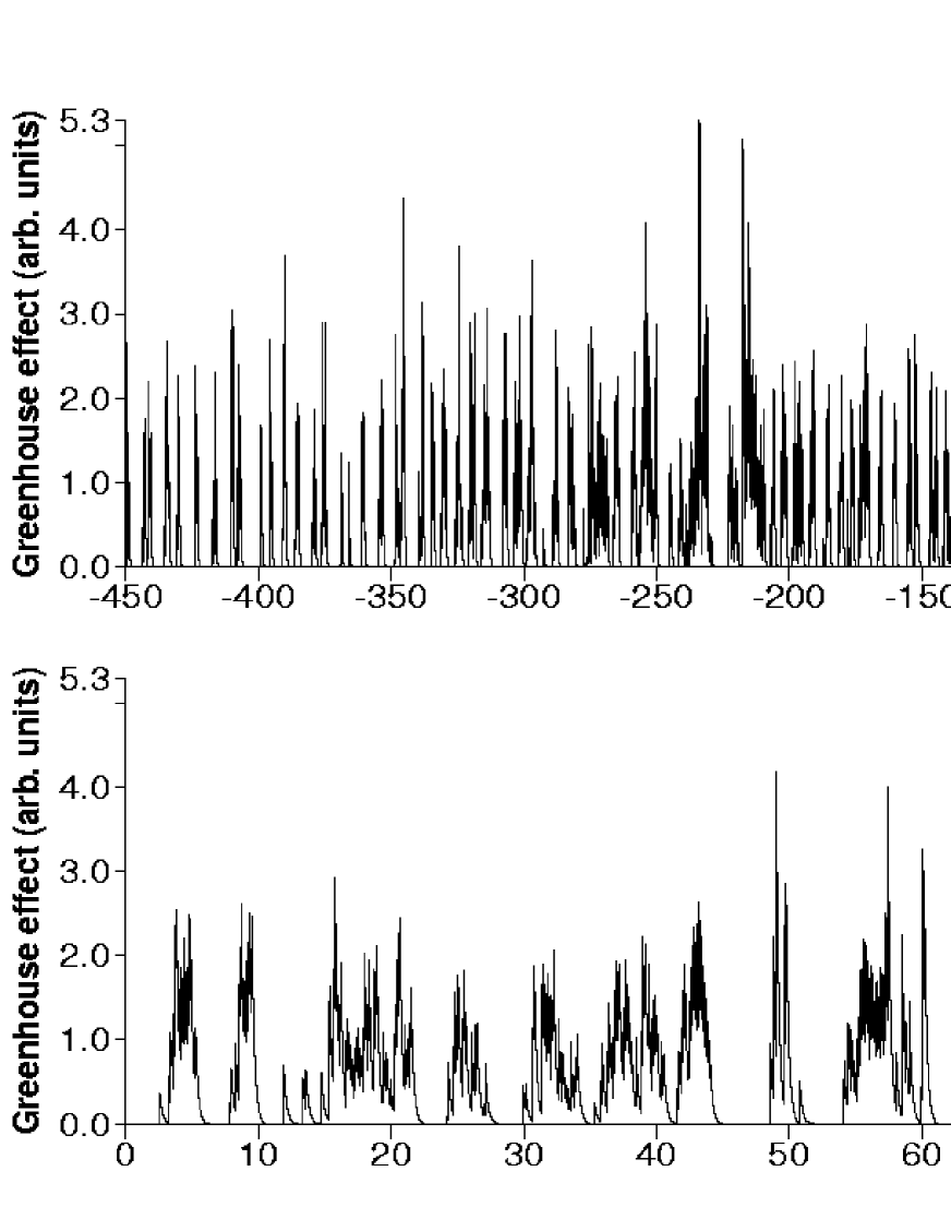
Figure 5: Upper panel: Greenhouse spectrum for the distance of closest approach pattern displayed in Fig. 3. The vertical scale is in arbitrary units. Lower panel: Expanded view of this spectrum over 150 kyr shows the similarity between the calculated structure and that of the Dansgaard-Oeschger events displayed in Fig. 1.

In order to determine the frequency spectrum of the Greenhouse signal presented in Fig. 5, we applied the Fast Fourier Transformation (FFT) algorithm to $2^{19}$ data points of this spectrum, i.e. to the time range from +150 to -374 kyr. The resulting power spectral density as a function of the reciprocal value of the frequency (the periodicity) is shown in Fig. 6. Distinct maxima can be seen at 6, 19, 23, and ca. 50, 90 and 175 kyr. These periodicities are the result of the interplay between the complex movement of Z’s and Earth’s orbital planes and should not be confused with similar values delivered by the Milankovitch theory. Here, the decisive parameters are the oscillation of both inclinations (about 7 kyr, and 100 kyr, respectively) and the movements of both perihelia [33]. In the high frequency domain these values compare quite well with those obtained from comparable analysis of the GRIP data displayed in Fig. 1. The peak observed at 90 kyr is close to the famous 100 kyr observed in the deep see sediment data. This suggest that the Interstadials might be the result of an enhanced clustering of the Dansgaard-Oeschger events. It should be noted, however, that such a comparison is problematic for two reasons: First of all, the results of our spectral analysis depend on the selected orbital parameters and in particular on the mass of Z. Therefore, we can only say that the evaluated periodicities of the postulated Greenhouse effect are not in contradiction with observation. Second, any comparison with deep sea sediment data is questionable, because the time scale of these measurements is usually tuned to the 100 kyr cycle of Earth’s orbital eccentricity.

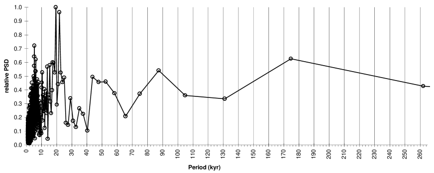
Figure 6: Power spectral density (PSD) of the Greenhouse spectrum presented in Fig. 5. Visible are three distinct peaks at 6, 19, 23 kyr, and three broad maxima at ca. 50, 90 and 175 kyr.

6 Earth’s past climate: a record of planet Z’s history

In chapter 1 we pointed to the strange fact that Earth’s climate was remarkably stable prior to the Ice Age epoch. Actually, the $\delta^{18}$O record of benthic foraminiferas from the Ocean Drilling program, site 659, shown in Fig. 7, suggests three different climate regimes for the last 5.0 Myr [9, 37].

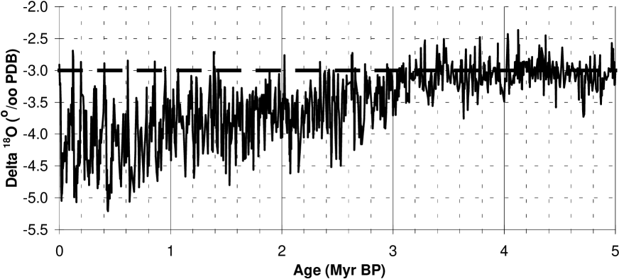
Figure 7: Benthic foraminifera $\delta^{18}$0 record from site 659 (18^∘ 05’N, 21^∘ 02’), according to Ref.[37]. This spectrum is a proxy for the extension and variation of the polar ice shields over the last 5.0 My. Increasing $\delta^{18}$O corresponds to decreasing ice caps and to warmer climate. The late Pliocene (before 3.2 Myr) is characterized by small ice caps and remarkably stable climatic conditions comparable to those of the Holocene. The corresponding value is shown by the horizontal dashed line.

The first phase is characterised by a very stable climate with small polar ice shields, and, in comparison with the following regimes, high temperature if it is assumed that ice extension and mean global temperature are correlated. This climate state is similar to that of the Holocene. A sudden drop in the global mean temperature terminated this state at about 3.2 Myr ago. In the following period the variability of the climate began to increase until about 1.0 Myr ago. At this time the proxy dates indicate a further drop of the mean temperature to the lowest known level in Earth history. This marks the beginning of the Ice Age epoch discussed in the previous chapter. It is obvious, that the properties of these three, or actually four different climate epochs, including the Holocene, cannot be explained in terms of the original Milankovitch theory, unless changes of solar irradiance or Earth’s orbital parameters according to observations are postulated. However, the introduction of such changes is hard to justify.

6.1 Some more polar shifts

In view of what has been derived so far the spectrum in Fig. 7 can be interpreted in a new way. Prior to about 3.3 Myr ago planet Z was inactive. If it existed, it was not yet on a highly eccentric orbit, cold, and without gas cloud. The climate was stable showing only the moderate changes which actually reflect the undisturbed Milankovitch effect. In agreement with this theory no 100 kyr-cycle appears up to this time [9]. The fact that the size of the continental ice caps during this period was comparable to the present day value indicate that Earth’s North pole was then located either in the Northern part of the Atlantic, in the Pacific Ocean, or at about the same position as it is today. It should be possible to evaluate its actual position using information on the climate in various regions during the Pliocene, and/or from geomagnetic field measurements. Around 3.2 Myr ago we assume that planet Z shifted Earth’s North pole towards the North American continent in the way described in chapter 3. As a consequence, the continental ice shields started to grow and with it Earth’s albedo, which reduced the global mean temperature. Of course, this implies that Z was on an eccentric Earth crossing orbit not later than at this time. Tidal heating consumed orbital energy so that its major semi-axis was slowly reduced. As mentioned in chapter 4, we are unable to decide in which way its eccentricity changed. The growing amplitudes of the climatic changes between about 3.2 and 1.0 Myr suggest a slowly growing gas cloud, which indicates an increasing orbital eccentricity. The tidal effects increased as well, which accelerated the heating up of Z. About 1.0 Myr ago, a second polar shift in direction toward the North American continent to the position assumed in chapter 3 further lowered the global temperature. The Ice Age epoch began. At this time the gas cloud was developed to its full size and the resulting Greenhouse heating created the temperature variations described in the previous chapter. A third and final polar shift terminated Earth’s Ice Age epoch 11.5 kyr ago, as discussed in chapter 3. The polar ice caps readjusted to the new position and, because of the diminishing size of the continental ice sheets, the global temperature increased during the early Holocene to its present value.

The suggestion that Earth’s pole was shifted at least three times during the last 3.2 Myr is compatible with the orbital calculations presented in chapter 4. They show that Z approached the Earth to polar shift distances about once in a million years, so that more than one shift event may be expected during the time range considered here. The direction of the polar shift depends on the geographic position of the closest approach. Antipode events excite the same directional shift, while those at positions differing by 180^∘ in longitude only, or positions with the same longitude but equal northern, respectively southern latitudes lead to opposite motions. The earlier shifts occured with encounters outside the Roche limit, which are more likely and, in view of the larger mass of Z at early times, sufficient to produce the required deformation.

6.2 On the origin and fate of planet Z

At this point it is tempting to speculate on the origin of Z. We see three possibilities: First, Z was originally on a hyperbolic trajectory but, during a close encounter with Jupiter, transferred to the required highly eccentric bound orbit. The major semi-axis $A$ of such an orbit would be larger than half of Jupiter’s orbital radius, i.e. $A>2.6$ AU, because of the presumably large initial velocity at the inflection point. Such a large $A$ is not compatible with our orbital calculations in chapter 4, which suggest $A\approx 1$ AU. Second, Z was originally a moon of Jupiter which was ejected due to the coupling with the other moons of Jupiter. Such an emission could result in a rather small initial velocity and accordingly to a highly eccentric orbit. Again, this is unlikely for the same reason as before. The last possibility relates to the Asteroid belt problem. It has been argued that the asteroids circling the sun at a mean distance of about 2.7 AU could be the remains of a collision between two larger bodies, one originally bound to the sun, the other presumably entering the solar system on a hyperbolic trajectory. Assuming that Planet Z was a reaction product of such a collision emerging with low velocity, then the major semi-axis of its orbit would be not much larger than about $A=1.35$ AU at the beginning of its journey around the sun. Considering the time required to reduce the orbital energy and to increase its eccentricity to the final values estimated in chapter 4, it is the most likely scenario.

It is open to discussion at what time Z disappeared. One possibility is that in the last close encounter it lost its angular momentum and plunged into the Sun. However, this requires an excentricity of not less than 0.98, and it supposes that the angular momentum received is opposed to the existing one. Therefore it seems more likely that the last encounter with the Earth was within the Roche limit, so that Z split into several parts. As a result of the reduced escape velocities of the debris, these parts lost material at an accelerated rate and were completely dissolved during the Holocene. The gas and dust clouds were expelled from the planetary system by radiation pressure.

7 A new understanding of Earth’s past climate

The previous chapters showed that the observed complex structure of Earth’s climate changes during the last few Million years can be explained in terms of a single object of planetary size, which was bound to the sun on a highly eccentric orbit for a limited time. This planet, called Z, was surrounded by a gas cloud and interacted gravitationally and through its gas cloud with the Earth and its atmosphere with a frequency determined by the pattern of its closest approaches to the Earth. These effects influenced Earth’s climate in two different ways.

Each polar shift event started with a huge flood, exceptionally strong winds, earthquakes and volcanic activities and ended with a displaced pole position after a couple of years. Following this shift the polar ice caps adjusted to the new pole position which changed Earth’s reflectivity, the albedo, and accordingly the global temperature. The new pole position determined whether this temperature was higher or lower after the shift. In agreement with observation we found that this happened about three times during the last 3.2 Myr. Two times the temperature dropped, suggesting that each time the pole was shifted closer towards the North American continent, so that the size of the continental part of the polar ice cap increased. During the last event, 11.5 kyr ago, it was moved into the arctic sea. At this position a net reduction of the polar ice caps prevailed. As a result of the reduced albedo, the global temperature increased to the presently known value. We also found that Z passed the Earth about 6 times in 100 kyr at distances less than 300 000 km. All of these flyby’s were close enough to excite large tides followed by earth quakes and volcanic activities. Recently, it has been suggested that the so called Heinrich events observed in the North Atlantic sediments during the last 100 kyrs — a rare, but distinct ice rafting phenomenon — could be the result of unusual, strong earthquakes [38, 39]. It is interesting to note that the observed 6 Heinrich-events per 100 kyr compare well with the predicted frequency for sub-lunar flybys.

The interaction between the gas cloud of Z and Earth’s atmosphere was quite spectacular as well, since most of the kinetic energy of the particles stopped in the upper atmosphere was converted into radiation. Probably, this radiation was intense enough to even ignite extended fires on Earth’s surface. After a couple of days the fires were extinct either by the flood, by heavy rain or by snow enriched with nitrous acid. When the atmosphere was cleared of the light absorbing components, the radiative forcing of the produced Greenhouse gases began to prevail, so that globally the temperature rapidly increased within a few years to the maximum value determined by the amount of Greenhouse gases produced during the encounter. The Greenhouse effect was a transient phenomenon, whose impact was limited by the amount of the Nitrogen compounds produced per encounter and the residence time of these gases. It may be responsible for the Dansgaard-Oeschger events observed during the Late Pleistocene. If so, then the Interstadials may be explained in terms of the quasi-periodic clustering of these events, as shown in chapter 5.2.

Summarizing, the many abrupt climate changes characterising Earth’s Ice Age epoch may reflect the interaction between Z and Earth during the last 3.2 Myr. These interactions were global catastrophes, the worst of which resulted in a polar wandering. These particular events even irreversibly changed Earth’s climate. The last polar shift event occurred only 11.5 kyr ago. As pointed out in chapter 2, the violence of this event is well documented by the observed sudden death of many animals, the extinction of some of the larger mammal species and the sudden rise of the sea level [14]. Possibly the traditions in old cultures of catastrophic events refer to the events mentioned above. Presently, we are enjoying a perfectly Milankovitch-driven moderate climate without the extreme and fast temperature variations observed prior to the last polar shift event. This may be due to the fact that planet Z is no longer influencing the Earth. We are confident that this new and pleasant climate state, called Holocene, shall last for an indefinite time, provided, we are willing to stop our own “Greenhouse attack” on Earth’s climate.

Although we have presented a consistent explanation of the complex structure of Earth’s climate variation during the last few Million years, we are aware that this rather exotic story has opened up more questions than it answered, because many of our arguments are based on considerations which are in terms of order of magnitude and very elementary. Nevertheless, we believe that this proposal merits further investigation, in view of its basic simplicity. In particular, we encourage state of the art calculations which could narrow the allowed parameter range of the hypothetical planet, or even disprove its existence. Of importance would be model calculations for the global climate for both pole position, with and without the suggested additional Greenhouse effect. Our static approach to Earth’s deformation during a fly-by should be replaced by a dynamical calculation. The actual amount of material that evaporates from a large body during its closest approach to the sun deserves a more detailed investigation. The sequence and efficiency of reactions initiated by an energetic atom, mostly Oxygen and Silicon, impinging on and stopped in the uppermost atmosphere, has to be further clarified, if necessary, with the help of appropriate experiments. A determination of the maximum age of the ice at the Siberian side of the Arctic and/or at the Atlantic side of the Antarctic could provide a test of the polar shift theory. Planet Z must have left its chemical signature in polar ice. The material was deposited in atomic or molecular form, in contrast to dust which is mainly of terresrial origin. Samples from the Moon could also reveal the presence of Z. These chemical traces might decide in which way Z disappeared from the solar system. If the dust cloud which envelops the inner solar system near the ecliptic plane originated from the last fragments of Z, then the intensity of the zodiacal light might show a measurable decrease in time [40]. We are optimistic, that the combined results of such studies will finally converge to a new understanding of Earth’s Ice Age epoch. A negative answer implies that the strange variability of the climate during this epoch, as well as the stepwise cooling of Earth’s climate beginning about 3.2 Mio years and its abrupt ending only 11.5 kyr ago remain unexplained. We are sceptical that these problems can be solved by means of any of the presently favoured Milankovich-based theories alone.

References

- [1] M.M. Milankovitch, Kanon der Erdbestrahlung und seine Anwendung auf das Eiszeitproblem, Königliche Serbische Akademie, Spez. Publikation No. 133 (1941) 1–633.
- [2] J. Imbrie, A. Berger, E.A. Boyle, S.C. Clemens, A. Duffy, W.R. Howard, G. Kukla, J. Kutzbach, D.G. Martinson, A. McIntyre, A.C. Mix, B. Molfino, J.J. Morley, L.C. Peterson, N.G. Pisias, W.L. Prell, M.E. Raymo, N.J. Shackleton, J.R. Toggweiler, On the structure and origin of major glaciation cycles, Paleoceanography, 8 (1993) 699–735.
- [3] J. Imbrie, J.D. Hays, D. Martinson, A. McIntyre, A. Mix, J. Morley, N. Pisias, W. Prell, N.J. Shackleton, The orbital theory of Pleistocene climate: support from a revised chronology of the marine O record, Milankovitch and Climate, Part I, (1984) 269–305 (eds. A.L. Berger et al).
- [4] R.A. Muller and G.M. McDonald, Glacial cycles and orbital inclination, Nature, 377 (1995) 107–108.
- [5] R. A. Muller and G. M. McDonald, Spectrum of 100 kyr glacial cycle: Orbital inclination, not eccentricity, Proc.Natl.Acad.Sci.USA 94, 8329–8334 (1997).
- [6] D. Paillard, The timing of Pleistocene glaciation from a simple multistage climate model, Nature, 391 (1998) 378–381.
- [7] A. Ganalpolski, St. Rahmsdorf, V. Peroukhov, M. Clausen, Simulation of modern and glacial climates with a coupled global model of intermediate complexity, Nature, 391 (1998) 351–356.
- [8] J.F. Adkins, E.A. Boyle, L. Keigwin, E. Cortigo, Variability of the North Atlantic thermohaline circulation during the last interglacial period, Nature, 390 (1997) 154–156.
- [9] R. Tiedemann, M. Sarntheim, N.J. Shackleton Astronomic time scale for the Pliocene Atlantic O and dust flux records of Ocean Drilling site 659, Paleoceanography, 9 (1994) 619–638.
- [10] Greenland Ice-core Project Members Climate instability during the last interglacial period recorded in the GRIP ice core, Nature, 364 (1993) 203–207.
- [11] P.M. Grootes, M. Stuiver, J.W.G. Johnson, J. Jouzel, Comparison of oxygen isotope records from the GISP2 and GRIP Greenland ice cores, Nature, 366 (1993) 552–554.
- [12] J.R. Petit, I. Basile, A. Leruyuet, D. Raynaud, C. Lorius, J. Jouzel, M. Sievenard, V.Y. Lipenkov, N.I. Barkov, B.B. Kudryashov, M. Davis, E. Saltzmann, V. Kotlyakov, Four climate cycles in Vostok ice core, Nature, 387 (1997) 359–360.
- [13] F. Stocker and D.G. Wright, Rapid changes in ocean circulation and atmospheric radiocarbon, Paleoceanography, 11 (1996) 773–795.
- [14] R.G. Fairbanks A 17’000-year glacio-eustatic sea level record: Influence of glacial melting rates on the Younger Drays event and deep-ocean circulation, Nature, 342 (1989) 637–642.
- [15] D. S. Fullerton, Stratigraphy and correlation of glacial deposits from Indiana to New York and New Jersey, Quaternary Science Reviews, 5 (1986) 23–36.
- [16] G. Gath Whitley, The Ivory Islands in the Arctic Ocean, J. of the Philosophical Society of Great Britain, XII (1910) 35.
- [17] G. Cuvier, Discours sur les révolutions de la surface du globe, et sur les changements qu’elles ont produit dans le règne animal, 1827.
- [18] W.B. Scott, A History of Land Mammals in the Western Hemisphere, ed. Mcmillan, New York, 1937.
- [19] O.S. Martin, Late Quaternary extinction: The promise of TAMS 14C-Dating, Nucl. Instr. Methods, B29 (1987) 179–186.
- [20] Charles H. Hapgood Earth’s shifting crust, ed. Pantheon Books, New York, 1958.
- [21] J.A. Clegg, M. Almond, P.H.S. Stubbs, Some sedimentary rocks in Britain, Philosphical Magazin, 45 (1954) 583–598.
- [22] T. Gold, Instability of the Earth’s axis of rotation, Nature, 175 (1955) 526–529.
- [23] A. Wegener, The origins of Continents and Oceans, Translated from the third German edition by J.G.A. Skerl, London, Methuen, 1924.
- [24] A.O. Kelly and F. Dachille, Target Earth, ed. Pensacola Engraving, Pensacola, Florida, 1953.
- [25] P. Melchior, The physics of the Earth’s core, ed. Pergamon Press, Oxford, England, 1986.
- [26] S.C. Chandler, On the variation of Latitude, The Astronomical Journal, XI, 249 (1891) 65–72.
- [27] S. Newcomb, On the Dynamics of the Earth’s Rotation with respect to the periodic variations of Latitude, Monthly Notes R. Astr. Soc. 52 (1892) 336–341.
- [28] W.H. Munk and G.J.F. Macdonald, The rotation of the Earth, A geophysical discussion, ed. Cambridge University Press, 1975.
- [29] J.M. Wahr, Computing tides, nutations and tidally-induced variations in the Earth’s rotation rate for a rotating elliptical Earth, Mitteilungen der geodätischen Institute der Technischen Universität Graz, 41 (1982) 327–336.
- [30] B.F. Chao, On the excitation of the Earth’s free wobble and reference frames, Geophys. J. R. Astron. Soc. 79 (1984) 555–563.
- [31] A. Geiger, private communication, Institut für Geodäsie und Photogrammetrie, ETH-Hönggerberg, CH-8093 Zürich.
- [32] M.L. Smith and F.A. Dahlen The period and Q of the Chandler wobble, Geophys. J. R. astron. Soc, 64 (1981) 223–281.
- [33] R. Nufer, W. Baltensperger and W. Woelfli, Long term behaviour of a hypothetical planet in a highly eccentric orbit, report available under http://xxx.lanl.gov/abs/astro-ph/9909464.
- [34] C. Flammarion Astronomie populaire, ed. F. Zahn, Neuchatel, 1880.
- [35] IPCC (1990): Scientific Assessment of Climate Change, Intergovernmental Panel on Climate Change, Report of Working Group I, WMO/UNEP, Geneva, 1990.
- [36] J.M. Barnola, D. Raynaud, Y.S. Korotkevich, C. Lorius, Vostok ice core provides 160’000-year record of atmospheric CO2, Nature, 329 (1987) 408–414.
- [37] S.C. Clemens and R. Tiedemann Eccentricity forcing of Pliocene-Early Pleistocene climate revealed in marin oxygene-isotope record, Nature, 385 (1997) 801–804.
- [38] H. Heinrich, Origin and consequences of cyclic ice rafting in the Northeast Atlantic Ocean during the past 130’000 years, Quaternary Resarch, 29 (1988) 142–152.
- [39] A.G. Hunt, P.E. Malin, Possible triggering of Heinrich events by ice-load-induced earthquakes, Nature, 393 (1998) 155–158.
- [40] B.Å.S. Gustafson, Physics of zodiacal dust, Annual Rev. Earth and Planet. Science, 22 (1994) 553–595.