International Journal of Modern Physics C,
c  World Scientific Publishing Company

1

SIMPLE AND EFFICIENT ALGORITHM FOR LARGE

SCALE MOLECULAR DYNAMICS SIMULATION

IN HARD DISK SYSTEM

MASAHARU ISOBE

Department of Physics, Kyushu University 33, Fukuoka 812-8581, Japan

E-mail: isobe@stat.phys.kyushu-u.ac.jp

Received 25 June 1999
Revised 21 July 1999

A simple and efficient algorithm of the molecular-dynamics simulation of the hard disk system based on the Event-Driven method is developed. From the analysis of algorithm, the complexity is ${\cal O}(\log N)$ per 1 event, and the constant coefficient of the complexity is smaller than conventional efficient algorithm based on the concept of Cell-Crossing Event. The maximum performance of more than 460 millions of collisions per CPU-hour on the Alpha600 compatible in a 2500 particle system is achieved. An extension to the infinite-space system based on this algorithm is also proposed.

Keywords: Event-Driven Molecular Dynamics; Hard Disk System; Algorithm.

1 Introduction

The molecular dynamics method (MD) was worked out in a paper for the first time by Alder and Wainwright in 1957,^? and they subsequently wrote a series of works.^?,?,? Their simulations were performed with many hard disks (or hard spheres in 3D) near the liquid-solid phase-transition point, and they found that the system was crystallized despite the particle had only repulsive force. These discoveries overturned the common opinion of those days, and greatly influenced the development of the study in computer simulations.

In the hard disk system, the dynamics consists of only collisions and straight-line movement. Since distinct events occur one after another in time, we do not need to integrate the differential equations with a constant time step based on Newton’s equation of motion. The method that is based on the finite constant time step and integration with the equations of particles step by step in time is sometimes called “Time-Step-Driven Molecular Dynamics” (TSDMD). On the other hand, in the hard disk system, the simulation that proceeds based on events is called “Event-Driven Molecular Dynamics” (EDMD). Compared with TSDMD simulation, the algorithm of EDMD simulation is completely different. We need the knowledge of an advanced algorithm and a data structure to perform the efficient simulation in EDMD. The strategy of direct computation of particle-pairs result in the complexity ${\cal O}(N^{2})$ for large particle number $N$. The point of improvement in the speed in hard disk system is how well we deal with the queue of a future event and the data structure.

The improvement of complexity in the algorithm of large-scale hard disk system was developed by Rapaport.^?,? This algorithm is based on the concept of sub-cell method,^? and both Collision Event and Cell-Crossing Event are stored into Multiple-Event Time List. Then the minimum time is searched by Binary Search Tree(BST).^? When the event occurs, the particle-pair or the particle — sub-cell respectively relevant to Collision Event or Cell-Crossing Event is deleted, and collision time for the particle relevant to the event is re-computed and new nodes are created. The BST is reconstructed by inserting these new nodes, and the minimum time is searched. On this algorithm, the averaged complexity per event becomes ${\cal O}(\log N)$, and the reduction of a large amount of computation is realized.

However, since the algorithm of Rapaport is very complicated and difficult to understand, several algorithms to simplify a data structure and improve the efficiency in the large-scale molecular dynamics simulation were proposed in the 90s.^?,?,? Marín et al.^? developed the technique of Local Minima Algorithm (LMA) to avoid additional re-computation for Event List. When we actually schedule future event list, LMA put only the minimum event time relevant to each particle into Complete Binary Tree (CBT). In 1995, Marín and Cordero^? compared various ${\cal O}(\log N)$ searching algorithms actually in EDMD simulation, systematically. They concluded that the efficiency of Complete Binary Tree (CBT) was the most suitable for hard disks system in all density regions. If the number of particles increases, for CBT it was clearly shown that efficiency increased significantly when compared with other searching algorithms. If one compare CBT with BST, their complexity are the same, i.e., ${\cal O}(\log N)$; but the algorithm of CBT is much simpler than that of BST, consequently CBT requires less memory space and realizes better actual performance.

In this paper, we developed an algorithm based on a strategy different from that of Cell-Crossing type. The algorithm is extended to Exclusive Particle Grid Method (EPGM) developed by Form et al.,^? (Sec. 2). Then, a bookkeeping method^? is applied (Sec. 3). Compared with the Cell-Crossing type, our algorithm extended the concept of Linked-Cell Method^?,? and Neighbor List, which are often used in TSDMD to carry out an efficient simulation.^? From the analysis of complexity, we show our algorithm is smaller than the complexity of Cell-Crossing type. By an empirical evaluation of the simulation in hard disk systems, our code could be shown to perform better than that of any previously-published works.

The infinite volume extension of the sub-cell method is usually considered impossible because the required memory is proportional to the volume in the conventional sub-cell method.^? We developed the method of compressing information about the infinite sub-cells into limited finite arrays. In addition, the hashing method, which is considered the most efficient searching algorithm, is applied to our method in order to pull out the information on a neighbor cell in high speed. It is found that the hashing method can be applied especially easily on our method.

Various applications in a very wide-ranging field will be possible by changing the external field and the collision rule in the large-scale EDMD. Typical examples performed by EDMD so far are: phase transition in the equilibrium system (solid-liquid transition and two-dimensional melting), ^?,?,?,? the nonequilibrium fluid system (e.g., Rayleigh-Bénard convection), ^?,? the nonequilibrium chemical-reaction system,^? the nonequilibrium dissipative system (granular system),^?,?,? random disk packing.^?,? When large-scale computation becomes possible in these systems, the value of simulation with a hard disk system must increase significantly.

The outline of this paper is as follows: in Secs. 2 and 3, the algorithms developed are explained. The comparisons with the algorithm of Cell-Crossing type by analyzing the complexities are shown in Sec. 4. The empirical evaluation is given in Sec. 5. The extension to the infinite system based on developed algorithms is explained in Sec. 6. In Sec. 7, a short summary and a final comment are presented.

2 Extended Exclusive Particle Grid Method

The sub-cell method is often used to achieve the significant reduction of computation. In the EDMD, the complexity of producing and updating future event list for restoring event time of each particle-pair are reduced to ${\cal O}(N)$ and ${\cal O}(1)$, respectively, by the sub-cell method. LCM is the method of dividing the system into small sub-cells. When the size of the sub-cell is bigger than a particle diameter, we will have a difficulty in coding a program, because we do not know how many particles enter in each sub-cell. Therefore, link lists must be prepared for the particles in each sub-cell.

On the other hand, another efficient sub-cell method, called Exclusive Particle Grid Method (EPGM), was independently developed by Buchholtz and Pöschel ^? and Form, Ito, and Kohring ^? to simulate the soft-core granular particle system in TSDMD. In this method, there is only one particle in each sub-cell. Though the EPGM is essentially the method of putting a particle to one sub-cell in LCM, it does not need to use pointers for neighbor sub-cells or link list. Here sub-cells in EPGM are called “grid”. In the EPGM, the length of grid $l_{gx}$ is determined by the following inequality:

$$\sigma<l_{gx}<\sqrt{2}\sigma,$$ (1)

where $\sigma$ is the radius of particle. One example of the number of grids $n_{gx},n_{gy}$ in the system of length $l_{x},l_{y}$ and the length of grid $l_{gx},l_{gy}$ can be calculated by the following equations.

$$l_{gx}=INT(l_{x}/(\sqrt{2}\sigma))+1$$ (2)

$$l_{gy}=INT(l_{y}/(\sqrt{2}\sigma))+1$$ (3)

$$n_{gx}=l_{x}/l_{gx}$$ (4)

$$n_{gy}=l_{y}/l_{gy}.$$ (5)

Note that the total number of grids is $n_{g}=n_{gx}\times n_{gy}$. As an analogy to the lattice spin system, EPGM is regarded as $N+1$-states Potts model of the square lattice system. This is because the particles are completely mapped into each lattice (i.e., one grid corresponds to one particle respectively), and we put 0 into the rest of grids in which there is no particle (Fig. 1). Since continuous and random positions of the particles are mapped into the lattice, the specification of neighbor particles becomes very easy.

Figure 1: A typical example of the mapping pattern using EPGM when packing fraction $\nu=0.70$. Both the position of hard disks and the occupied lattices are shown.

Form et al.^? applied this algorithm in the high-density soft-core granular system with short-distance interaction in TSDMD. They achieved high efficiency on a vector computer. Based on this algorithm, the extension of EPGM to EDMD in the hard disk system is developed.

When the system is in high-density, EPGM can be simply applied to EDMD. For a candidate of the next colliding particle-pairs, we need to search only 24 neighbor grids, which form the square mask. If neighbor grid is not 0, the collision times of candidates of colliding particle-pairs are computed only by the registered particle number in the square mask. We call these 24 neighbor grids MIN, because this is the minimum mask in the simulation of EDMD. Note that if the smaller mask is used, the computation will break down during the simulation, since a possibility of overlap between a central particle in the mask and particles outside the mask occurs. When EPGM is applied in the high-density system, the computation is optimized because a sufficient number of particles contained in the mask MIN. These are enough to be candidates of particle-pairs of collision, and only the required particles are registered in the mask MIN; the efficiency increases as a result of the computational reduction of collision time for neighbor particle-pairs.

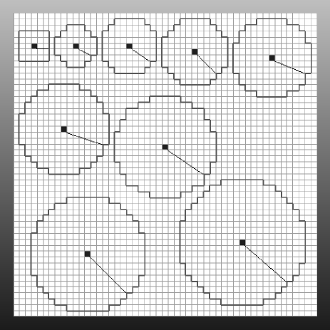
Figure 2: Minimum mask (MIN) and larger masks, which are generated by the algorithm of making circle on the computer display, are shown. The solid lines in each mask denote the minimum distance from the central lattice of mask to the frame of mask.

On the other hand, when the system is of low density, no sufficient number of particles as candidates of collision are registered in the mask MIN. Under such a situation, the computation will break down, since collision time between the central particle in the mask and particles out of the mask will become the next minimum time. In order to prevent this breakdown, the extension of EPGM is developed. The region must be extended to look for candidates of collision particle-pairs bigger than MIN. Since the rigorous isotropy of neighbors in EDMD is not necessarily demanded, the shape of the mask might be approximated by a rough circle. It is found that the mask approximated by the lattice-like grid with the circle can use the algorithm describing the circle on the discrete space of computer display. Figure 2 displayed the circles from R= 3 to R= 10 on the discrete space of computer display, which MIN is also showed over Fig. 2. The total number of neighbor grids (mask) are 24 (MIN), 36 (R=3), 68 (R=4), 96 (R=5), 136 (R=6), 176 (R=7), 224 (R=8), 292 (R=9), 348 (R=10), respectively. This extension of EPGM is called Extended Exclusive Particle Grid Method (EEPGM).

Compared with LCM, EEPGM is simple, because rough neighbor particles can be simply regulated by grids so that only the necessary minimum may be taken. In EEPGM, since link list and pointers for neighbor sub-cell is not necessary, the required memory is also sharply reduced, the number of operations for setting EEPGM is small, and the program becomes very simple. Moreover, the extension to the infinite volume system is easy when using a hashing method to EEPGM. This is explained in detail in Sec. 6.

3 Neighbor List and Dynamical Upper Time Cut-Off

Though EEPGM produces a significant reduction of computation compared with considering all particle-pairs, it is inadequate when large number of particle simulation are performed. In this section, the next step in the strategy of the increase in efficiency based on EEPGM is developed. Here, the concept of Neighbor List (NL)^? is adopted. Since the grids correspond to each particle, we can regard the registration of Neighbor List as already being completed. Therefore, we need only to search neighbor particles along in the form of a mask.

In the usual way of LCM+NL, after the system is divided into sub-cells, particles are listed into the link list. Then neighbor particles within radius $r_{NL}$ are entered into Neighbor List from the link list. However, since the length of both lists is unknown, they must be estimated by trial and error. Although registration of NL is completed by one operation in EEPGM, LCM+NL must use two different unknown size lists, which is accompanied by a complicated procedure and requires difficult programming. Therefore, EEPGM (+NL) is simple, which means that both debugging and extension do not require excessive effort; moreover, only the minimum nearest particles can be seen, because the system is divided into the minimum sub-cells, i.e., the grid. Since registration of NL is completed by one operation in EEPGM, efficiency is better than LCM+NL at a result.

The next improvement in speed is that the computation of collision time only from particle-pairs which are registered in the mask of EEPGM during the time $t_{NL}$. Then the complexity of EEPGM for every event is reducible to ${\cal O}(1)$ instead of ${\cal O}(N)$. After time $t_{NL}$, the grids are again re-mapped in order to update neighbor particles. The time of Neighbor List $t_{NL}$ must be determined such that the central particle does not collide with a particle completely out of the mask. If $t_{NL}$ is too long and such a event happens, the program picks up a wrong pairs of particles to collide, which could result in negative collision time. This conventional determination of $t_{NL}$ needs a lot of trial and error. In order to overcome these difficulties, $t_{NL}$ is determined by the following procedure. First, after completing EEPGM, the maximum velocity $v_{max}$ in the system is searched, and the value of its velocity is restored (the complexity of this searching is the same order of EEPGM ${\cal O}(N)$). Next, time $t_{NLmin}$ of the system is calculated. In this calculation we suppose both the central particle and the particle out of the mask have the maximum velocity and those particles undergo head-on collision. If $t_{NL}=t_{NLmin}$, a counting mistake of collision pairs in the system never occurred during the time $t_{NLmin}$. The minimum NL distance $r_{NLmin}$ is required when $t_{NLmin}$ is calculated, which becomes clear from the geometry of the adopted mask shown in Fig. 2. Therefore, $t_{NLmin}$ is given by

$$t_{NLmin}=\frac{r_{NLmin}-2\sigma_{max}}{2v_{max}}$$ (6)

where $\sigma_{max}$ is the maximum radius of particle in the system. The minimum distances $r_{min}$ for each mask are shown in Table 1.

	MIN.	R=3	R=4	R=5	R=6	R=7	R=8	R=9	R=10
$r_{min}/l_{gx}$	$2$	$\sqrt{5}$	$\sqrt{13}$	$\sqrt{18}$	$\sqrt{29}$	$\sqrt{40}$	$\sqrt{52}$	$\sqrt{72}$	$\sqrt{85}$

Table 1: The minimum distance for each mask.

When we simulate in the equilibrium system, this strategy will work well because $t_{NLmin}$ hardly changes. However, in the nonequilibrium system (e.g., the relaxing process or the system with heat bath) it breaks down because the maximum velocity changes drastically at every step. To overcome this difficulty, we must check the maximum velocity for each event with energy increase. Fortunately the complexity of this checking process is ${\cal O}(1)$. Therefore, in the simulation of the nonequilibrium system $t_{NL}$ will change one after another. We call this change in $t_{NL}$ techniques Dynamical Upper Time Cut-off (DUTC). The development of DUTC, EEPGM became applicable in the nonequilibrium system.

Although we do not need to update the grid pattern for a long time in the high-density system, we should often do so when we use the mask MIN in low-density systems because the grid pattern changes drastically. In order to reduce the frequency of updating grid pattern, we can only use a bigger mask.

4 Analysis of Complexity

Analysis of complexity is one of important factor in estimating the efficiency of algorithms. In this section, a comparison of analysis of complexity between the algorithm of the Cell-Crossing type and the EEPGM + DUTC is shown. The difference between the algorithm of Cell-Crossing type and the strategy of EEPGM + DUTC is Cell-Crossing Event itself. Therefore, especially with regard this point, both complexities with a constant coefficient $k$ are estimated in the case of $A\times N$ collisions being actually simulated. Note that the particle number $N$ is supposed to be quite a large number and the techniques of improvement in the speed are also used in both algorithms described by Marín et al.,^?

• Cell-Crossing type (LCM + Cell-Crossing Event)

  • The initial and last step ($\times 1$)

    Linked-Cell Method — $k_{LCM}\times N$

    Computation of Event Time — $k_{PP}\times 9\times N_{c}\times N+k_{PC}\times 4\times N$

    Construction of Complete Binary Tree — $k_{CBT}\times N$

    Update the final position of particles — $k_{UPDATE}\times N$

  • Iteration Step (loop)

    $(A\times N)\times(k_{PP}\times 9\times N_{c}+k_{CBT}\times\log N)+(B\times N)\times(k_{PC}\times 3+k_{CBT}\times\log N)$

  where $N_{c}$ is the number of particles per sub-cell. The most important point is that the Cell-Crossing Event occurs at a certain ratio to Collision Events. Therefore, the additional computation of $B\times N$ times Cell-Crossing Events are needed when we want to simulate $A\times N$ times Collision Events. Since the complexity of the terms related to Cell-Crossing Events is always ${\cal O}(N)$, this is not negligible in the actual simulation.

• EEPGM + DUTC

  • Update of EEPGM ($\times C$)

    EEPGM — $k_{EEPGM}\times N$

    Computation of Event Time — $k_{PP}\times N_{g}\times N$

    Search the Maximum Velocity — $k_{MVS}\times N$

    Construction of Complete Binary Tree — $k_{CBT}\times N$

    Update the final position of particles — $k_{UPDATE}\times N$,

  • Iteration Step (loop)

    $(A\times N)\times(k_{PP}\times N_{g}+k_{CBT}\times\log N)$

  where $N_{g}$ is the averaged particle number of the mask. Actually the value of $C$ is an order $C\sim A$, which is the same order of the frequency of updating EEPGM.

Now, the comparison with order $N$ in both algorithm with constant coefficient is as follows:

• Cell-Crossing type

  $(k_{LCM}+k_{PP}\times 9\times N_{c}\times(A+1)+k_{PC}\times(3\times B+1)+k_{CBT}+k_{UPDATE})\times N+(A\times k_{CBT}+B\times k_{CBT})\times N\times\log N$

• EEPGM + DUTC

  $(k_{EEPGM}+k_{PP}\times 2\times N_{g}+k_{MVS}+k_{CBT}+k_{UPDATE})\times C\times N+(A\times k_{CBT})\times N\times\log N$

The most striking point is that the complexity of Cell-Crossing Events is of order of ${\cal O}(N\log N)$ (i.e., $B\times k_{CBT}\times N\times\log N$). This result of analysis suggest that the efficiency of EEPGM + DUTC is better than for Cell-Crossing when the simulation with an enormous number of particle is performed. On the other hand, in the comparatively small particle system, the coefficient of $C\times N$ terms in EEPGM + DUTC may be larger than Cell-Crossing type. However, the difference might be quite small, and it is impossible to estimate an exact coefficient of algorithms analytically. To the author’s knowledge, the coefficient of $N$ terms is strongly dependent on the ratio of $N_{c}$ to $N_{g}$, and the rough estimation shows both algorithms are same when $N_{g}/N_{c}\sim 4$. Actually, the increase in computing the Cell-Crossing Events has almost no effect to the CPU time as the simulation is actually performed in a system with a very large number particles.

5 Empirical Evaluation

When actually running the simulation, the order of the complexity is not so reliable, because it depends strongly on a constant coefficient when the number of the particle is relatively small. Moreover, the efficiency of the code changes significantly by the ability of a computer, the language, the performance of compiler, and the ability of programmers. Though a perfect comparison of efficiency of codes developed by the past workers is impossible, some publications showed how many particle collisions per CPU-hour can their codes be computed by their computers.

Marín et al.^? simulated with hard disk system, and they also compared their code with the codes based on two main high-speed algorithms proposed by Rapaport ^? and Lubachevsky,^? respectively. As a result, it was shown that the efficiency of the code of Marín et al. was higher for the entire density region. Therefore, the code proposed here should be compared with the code of Marín et al., and is computed with equal number of particles ($N=2,500$). Marín et al. achieved the maximum performance of 16.07 millions of collisions per one CPU hour on a SUN690 workstation. Note that only the highest performance is shown because it is different for different densities of the systems. On the other hand, the code proposed here achieved a maximum performance of 460 million collisions per one CPU hour (Alpha600 compatible, DEC-Fortran). It was found that a high efficiency was realized even if the performance of the machine was reduced.

Note that the workstation of our laboratory could actually simulate a 2,500,000 particle system. In this simulation, the amount of installed memory was $250$ megabytes and the computation performance was 210 million collisions per one CPU hour.

6 Extension to Infinite Volume System

In this section, a simple example in the open boundary system that does not have a ceiling is considered. This is the case when there is an energy source at the bottom of the system under uniform gravity.

The system is also divided into grids by EEPGM. However, because the top of the system is open, the grid goes to the top of the system infinitely. This means that the number of arrays for the grid becomes infinity, and the simulation is impossible from finite memory. To overcome this difficulty, the hashing method, which is well known as the fastest searching algorithm, is applied to keep the number of arrays in finite size and to simulate the dynamics of the system with high-efficiency.

• Construction of Data Structure

  Firstly, the serial number of grid $N_{G}(i_{g},j_{g})$ is defined by

  $$N_{G}=N_{gx}(j_{g}-1)+i_{g},$$ (7)

  where $N_{gx}$ and $i_{g}(1\leq i_{g}\leq N_{gx})$ are the total number of grids and the index of grid in the horizontal direction, respectively; $j_{g}(1\leq j_{g}\leq\infty)$ refers to the index of grid in the vertical direction. In addition, the maximum number of the serial grid $N_{Gmax}$ is calculated by $N_{Gmax}=N_{gx}(j_{gmax}-1)+i_{gmax}$; the pair $(i_{gmax},j_{gmax})$ is at the maximum grid pair of containing the particle.

  The serial grid $N_{G}(1\leq N_{G}\leq N_{Gmax})$ is a one-dimensional array, in which particle number or $0$ is listed. This is called the one-dimensional Virtual Array. When $j_{max}$ is large value, there are many $0$’s in the one-dimensional Virtual Array. Though there is only information that a particle is not just in grid, this $0$ relates to the memory capacity directly. Now Virtual Array is compressed. After all, the only information necessary is the particle number and its index of grid. Therefore, one-dimensional integer arrays are prepared for $A(N),BX(N),BY(N)$, and grids of $0$ in Virtual Array are ignored, and then packed in order from the end; $A(N)$ stores the particle numbers only, and $BX(N)$ and $BY(N)$ stores indexes of $i_{g}$ and $j_{g}$ for each particle, respectively. If you want to know whether there is a particle in grid $(i^{\prime}_{g},j^{\prime}_{g})$, you need only search the index-pairs correspond to $(i^{\prime}_{g},j^{\prime}_{g})$ in the lists of $BX(N),BY(N)$ linearly. However, this process is inefficient because the complexity of ${\cal O}(N)$ is necessary in searching.

  Therefore, the hashing method, otherwise known as an algorithm which can realize the searching with ${\cal O}(1)$ is applied. The following simplest hashing function is explained here as an example though various hashing functions can be considered and there is still room for development.

  First, a hashing function is defined by

  $$k=INT(\frac{N_{G}-1}{L})+1$$ (8)

  which means that the Virtual Array is equally divided by the length $L$ (e.g., $5\sim 10$) and key $k$ is calculated corresponding to serial number $N_{G}$. Then, $k_{max}=INT(N_{Gmax}/L)$ is calculated using $N_{Gmax}$. Then additional arrays $C(k_{max}),D(k_{max})$ are prepared, these arrays are restored in $C(k)$ where $k$ begins in $A(N)$ and in $D(k)$ how big the arrays for each $k$. In this case, necessary arrays are $A(N),BX(N),BY(N),C(k_{max}),D(k_{max})$, and these are confined to a finite value. Since additional arrays needed to use the hashing method are only $C(k_{max}),D(k_{max})\ (k_{max}<N$), the amount of memory used is only slightly increased in comparison with the linear searching.

• Searching Process

  In order to know what the particle number is in the grid ($i^{\prime}_{g},j^{\prime}_{g}$), the following process is carried out. First, a serial number is calculated by $N^{\prime}_{G}=N_{gx}(j^{\prime}_{g}-1)+i^{\prime}_{g}$. Next, $k^{\prime}$ is calculated by the equation of hashing function (8). Then, the searching ranges of $BX,BY$ are limited only to index of [$C(k^{\prime})\sim C(k^{\prime})+D(k^{\prime})-1$] ($\leq L$). If there are equal pairs of grids ($i^{\prime}_{g},j^{\prime}_{g}$) as a result of the searching of $BX,BY$, the index $s$ of $BX,BY$ reveals $A(s)$, which is the particle number in the grid ($i^{\prime}_{g},j^{\prime}_{g}$). When equal pair is not found in $BX,BY$, there is no particle in the grid.

  This procedure becomes possible in high-speed simulation. The complexity becomes ${\cal O}(1)$ instead of the linear search ${\cal O}(N)$, because a search is only carried out on the length of $L$ with hashing method.

A computation is possible for other boundary conditions with the same procedure if one-dimensional Virtual Array can be created. Therefore, high-speed simulation is possible in principle for any kind of boundary to be applied. There is room for improvement in hashing functions, which is the easiest when dividing equally, because it is obviously inappropriate when particles are distributed heterogeneously.

The strategy of EEPGM has an advantage that it is easily extended. The ease of a development is an important factor of the evaluation of an algorithm.

One problem in low-density systems is the overwhelming increase of the arrays assigned to grid in comparison to the number of the particles. This is not desirable as the memory capacity is the same of as that of infinite system. However, the arrays for the grid are compressed to the size of the particle number in the same way as described above. Since supplementary arrays are made by the hashing method and information on neighboring grids is efficiently obtained, there is no problem for both efficiency and memory capacity.

7 Concluding remarks

In this paper, we developed an algorithm for a hard disk system without using Cell-Crossing Event, which is simple, efficient and easy to extend. EEPGM can be easy to extend because of its simplicity, which can never be realized in LCM. One example is the system that hard disks with various size of diameters coexist. Though there was a limitation in the degree of the poly-dispersion with EPGM described to Buchholtz and Pöschel, ^? EEPGM can be applied easily to those systems. First, the grid is made based on the smallest particle radius in the system. Next, we have only to check the nearest grids by using a suitable mask of the bigger level when the poly-dispersity increases. This way, EEPGM has a wider application than EPGM.

This code achieved the fastest simulation speed in the world; about 460 million of collisions per CPU hour for the 2500 disk system on the VT-Alpha-600. Since the order of complexity is ${\cal O}(\log N)$, the increase of complexity is slow when the particle number increases. Now, we can carry out large-scale molecular dynamics simulation $(\sim 10^{6})$ on the usual Workstation in our laboratory.

Hard particle simulation is a powerful tool for studying the fluidized state described by the kinetic theory or hydrodynamics. Therefore, the large-scale simulation in the hard particle system will become an important subject.

Finally, the algorithm in this paper is suitable for the scalar machine, and the development of an algorithm for the parallel machine is the subject of a future study. Note that we discuss only hard disk systems in 2D for simplicity, but an extension to hard spheres system in 3D is easy to be carried out.

Acknowledgements

The auther thanks Prof. Nakanishi for reading the manuscript and making a number of helpful suggestions. He also gratefully acknowledge helpful discussions with Dr. Muranaka on several points in the paper. A part of the computation in this work was done by the facilities of the Supercomputer Center, Institute for Solid State Physics, University of Tokyo.

References

References

- [1] B. J. Alder and T. E. Wainright, J. Chem. Phys. 27, 1208 (1957).
- [2] B. J. Alder and T. E. Wainright, J. Chem. Phys. 31, 459 (1959).
- [3] B. J. Alder and T. E. Wainright, J. Chem. Phys. 33, 1439 (1960).
- [4] B. J. Alder and T. E. Wainright, Phys. Rev. 127, 359 (1962).
- [5] D. C. Rapaport, J. Comput. Phys. 34, 184 (1980).
- [6] D. C. Rapaport, The art of molecular dynamics simulation (Cambridge University Press, Cambridge, 1995).
- [7] J. J. Erpenbeck and W. W. Wood, in Modern Theoretical Chemistry Vol.6, Statistical Mechanics Part B, ed. B.J.Berne (Plenum, New York, 1977), Chap. 1, p. 1.
- [8] D. E. Knuth, Sorting and Searching, The Art of Computer Programming, Vol.3, (Addison-Wesley, Reading, Mass., 1973).
- [9] B. D. Lubachevsky, J. Comput. Phys. 94, 255 (1991).
- [10] K. Shida and Y. Anzai, Comput. Phys. Commun. 69, 317 (1992).
- [11] A. T. Krantz, ACM Trans. Model. Comput. Sim. 6, 185 (1996).
- [12] M. Marn, D. Risso, and P. Cordero, J. Comput. Phys. 109, 306 (1993).
- [13] M. Marn and P. Cordero, Comput. Phys. Commun. 92, 214 (1995).
- [14] V. Buchholtz and T. Pschel, Int. J. Mod. Phys. C4, 1049 (1993).
- [15] W. Form, N. Ito, and G. A. Kohring, Int. J. Mod. Phys. C4, 1085 (1993).
- [16] L. Verlet, Phys. Rev. 159, 98 (1967).
- [17] B. Quentrec and C. Brot, J. Comput. Phys. 13, 430 (1975).
- [18] R. W. Hockney and J. W. Eastwood, Computer Simulation Using Particles (McGraw-Hill, New York, 1981).
- [19] M. P. Allen and D. J. Tildesley, Computer Simulation of Liquids (Clarendon Press, Oxford, 1987).
- [20] M. Mareschal, M. Malek-Mansour, A. Puhl, and E. Kestemont, Phys. Rev. Lett. 41, 2550 (1988).
- [21] D. C. Rapaport, Phys. Rev. Lett. 60, 2480 (1988).
- [22] T. Kawakatsu and A.Ueda, J. Phys. Soc. Jpn. 56, 847 (1987).
- [23] I. Goldhirsch and G. Zanetti, Phys. Rev. Lett. 70, 1619 (1993).
- [24] S. McNamara and W. R. Young, Phys. Rev. E53, 5089 (1996).
- [25] C. Bizon, M. D. Shattuck, J. B. Swift, W. D. McCormick, and H. L. Swinney, Phys. Rev. Lett. 80, 57 (1998).
- [26] B. D. Lubachevsky and F. H. Stillinger, J. Stat. Phys. 60, 561 (1990).
- [27] B. D. Lubachevsky, F. H. Stillinger, and E. N. Pinson, J. Stat. Phys. 64, 501 (1991).