2D Numerical Simulation of the Resistive Reconnection Layer.

Abstract

In this paper we present a two-dimensional numerical simulation of a reconnection current layer in incompressible resistive magnetohydrodynamics with uniform resistivity in the limit of very large Lundquist numbers. We use realistic boundary conditions derived consistently from the outside magnetic field, and we also take into account the effect of the backpressure from flow into the the separatrix region. We find that within a few Alfvén times the system reaches a steady state consistent with the Sweet–Parker model, even if the initial state is Petschek-like.

PACS Numbers: 52.30.Jb, 96.60.Rd, 47.15.Cb.

Magnetic reconnection is of great interest in many space and laboratory plasmas [1, 2], and has been studied extensively for more than four decades. The most important question is that of the reconnection rate. The process of magnetic reconnection, is so complex, however, that this question is still not completely resolved, even within the simplest possible canonical model: two-dimensional (2D) incompressible resistive magnetohydrodynamics (MHD) with uniform resistivity $\eta$ in the limit of $S\rightarrow\infty$ (where $S=V_{A}L/\eta$ is the global Lundquist number, $L$ being the half-length of the reconnection layer). Historically, there were two drastically different estimates for the reconnection rate: the Sweet–Parker model [3, 4] gave a rather slow reconnection rate ($E_{\rm SP}\sim S^{-1/2}$), while the Petschek [5] model gave any reconnection rate in the range from $E_{\rm SP}$ up to the fast maximum Petschek rate $E_{\rm Petschek}\sim 1/\log S$. Up until the present it was still unclear whether Petschek-like reconnection faster than Sweet–Parker reconnection is possible. Biskamp’s simulations [11] are very persuasive that, in resistive MHD, the rate is generally that of Sweet–Parker. Still, his simulations are for $S$ in the range of a few thousand, and his boundary conditions are somewhat tailored to the reconnection rate he desires, the strength of the field and the length of layer adjusting to yield the Sweet–Parker rate. Thus, a more systematic boundary layer analysis is desirable to really settle the question.

We believe that the methods developed in the present paper are rather universal and can be applied to a very broad class of reconnecting systems. However, for definiteness and clarity we keep in mind a particular global geometry presented in Fig. 1 (although we do not use it explicitly in our present analysis). This Figure shows the situation somewhere in the middle of the process of merging of two plasma cylinders. Regions I and II are ideal MHD regions: regions I represent unreconnected flux, and region II represents reconnected flux. The two regions I are separated by the very narrow reconnection current layer. Plasma from regions I enters the reconnection layer and gets accelerated along the layer, finally entering the separatrix region between regions I and II. In general, both the reconnection layer and the separatrix region require resistive treatment.

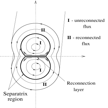
FIG. 1.: The global geometry.

In the limit $S\rightarrow\infty$ the reconnection rate is slow compared with the Alfvén time $\tau_{A}=L/V_{A}$. Then one can break the whole problem into the global problem and the local problem [6]. The solution of the global problem is represented by a sequence of magnetostatic equilibria, while the solution of the local problem (concerning the narrow resistive reconnection layer and the separatrix region) determines the reconnection rate. The role of the global problem is to give the general geometry of the reconnecting system, the position and the length of the reconnection layer and of the separatrix, and the boundary conditions for the local problem. These boundary conditions are expressed in terms of the outside magnetic field $B_{y,0}(y)$, where $y$ is the direction along the layer. In particular, $B_{y,0}(y)$ provides the characteristic global scales: the half-length of the layer $L$, defined as the point where $B_{y,0}(y)$ has minimum, and the global Alfvén speed, defined as $V_{A}=B_{y,0}(0)/\sqrt{4\pi\rho}$.

In the present paper we study the local problem using the boundary conditions provided by our previous analysis of the global problem [7]. Our main goal is to determine the internal structure of a steady state reconnection current layer (i.e., to find the 2D profiles of plasma velocity and magnetic field), and the reconnection rate represented by the (uniform) electric field $E$. We assume incompressible resistive MHD with uniform resistivity. Perfect mirror symmetry is assumed with respect to both the $x$ and $y$ axes (see Fig. 2).

This physical model is described by the following three steady state fluid equations: the incompressibility condition, $\nabla\cdot{\bf v}=0$, the $z$ component of Ohm’s law, $\eta j_{z}=E+[{\bf v}\times{\bf B}]_{z}$, and the equation of motion, ${\bf v}\cdot\nabla{\bf v}=-\nabla p+[j_{z}\hat{z}\times{\bf B}]$ (with the density set to one).

Now we take the crucial step in our analysis. We note that the reconnection problem is fundamentally a boundary layer problem, with $S^{-1}$ being the small parameter. This allows us to perform a rescaling procedure [8] inside the reconnection layer, to make rescaled resistivity equal to unity. We rescale distances and fields in the $y$-direction by the corresponding global values ($L$, $B_{0,y}(0)$, and $V_{A}$), while rescaling distances and fields in the $x$-direction by the corresponding local values: $x\rightarrow x\delta_{0}$, $v_{x}\rightarrow v_{x}V_{A}\delta_{0}/L$, $B_{x}\rightarrow B_{x}B_{y,0}(0)\delta_{0}/L$, $E\rightarrow EB_{y,0}(0)V_{A}\delta_{0}/L$. Here, $\delta_{0}\equiv LS^{-1/2}$ is the Sweet-Parker thickness of the current layer. Thus, one can see that the small scale $\delta_{0}$ emerges naturally. Then, using the small parameter $\delta_{0}/L=S^{-1/2}\ll 1$, one obtains a simplified set of fluid equations for the rescaled dimensionless quantities:

$$\nabla\cdot{\bf v}=0,$$

$$E={{\partial B_{y}}\over{\partial x}}-v_{x}B_{y}+v_{y}B_{x},$$

(where the first term on the right hand side (RHS) is the resistive term) and

$${\bf v}\cdot\nabla v_{y}=-{{\partial p}\over{\partial y}}+B_{x}{{\partial B_{y}}\over{\partial x}}.$$

In the last equation (representing the equation of motion in the $y$-direction, along the current layer) the pressure term can be expressed in terms of $B_{y}(x,y)$ and the outside field $B_{0,y}(y)$ by using the vertical pressure balance (representing the $x$-component of the equation of motion, across the current layer):

$$p(x,y)={{B_{y,0}^{2}(y)}\over 2}-{{B_{y}^{2}(x,y)}\over 2}.$$

We believe that this rescaling procedure captures all the important dynamical features of the reconnection process.

The problem is essentially two-dimensional, and requires a numerical approach. Therefore, we developed a numerical code for the main reconnection layer, supplemented by another code for the separatrix region. The solution in the separatrix region is needed to provide the downstream boundary conditions for the main layer (see below).

The steady state was achieved by following the true time evolution of the system starting with initial conditions discussed below. The time evolution was governed by two dynamical equations:

$$\dot{\Psi}=-\nabla\cdot({\bf v}\Psi)+{{\partial^{2}\Psi}\over{\partial x^{2}}}+\left(\eta_{y}{{\partial^{2}\Psi}\over{\partial y^{2}}}\right),$$

$$\dot{v_{y}}=-\nabla\cdot({\bf v}v_{y})-{d\over{dy}}\left[{{B_{y,0}^{2}(y)}\over 2}\right]+\nabla\cdot({\bf B}B_{y})+\left(\nu_{y}{{\partial^{2}v_{y}}\over{\partial y^{2}}}\right).$$

(Small artificial resistivity $\eta_{y}$ and viscosity $\nu_{y}$ were added for numerical stability.) The natural unit of time is the Alfvén time $\tau_{A}=L/V_{A}$. The magnetic flux function $\Psi$ is related to ${\bf B}$ via $B_{x}=-\Psi_{y}$, and $B_{y}=\Psi_{x}$. At each time step, $v_{x}$ was obtained by integrating the incompressibility condition: $v_{x}(x,y)=-\int_{0}^{x}(\partial v_{y}/\partial y)dx$. Note that this means that we do not prescribe the incoming velocity, and hence the reconnection rate: the system itself determines how fast it wants to reconnect.

We used the finite difference method with centered derivatives in $x$ and $y$ (second order accuracy). The time derivatives were one-sided. The numerical scheme was explicit in the $y$ direction. In the $x$ direction the resistive term $\partial^{2}\Psi/\partial x^{2}$ was treated implicitly, while all other terms were treated explicitly. Calculations were carried out on a rectangular uniform grid. We considered only one quadrant because of symmetry (see Fig. 2). More details can be found in Ref. [9].

FIG. 2.: Computational box used in the numerical simulation.

The boundary conditions on the lower and left boundaries were those of symmetry (see Fig. 2). On the upper (inflow) boundary $x=x_{\rm lim}$ the boundary conditions were $\partial v_{y}/\partial x=0$ (which worked better than $v_{y}=0$) and $B_{y}(x_{\rm lim},y)=B_{0,y}(y)$ — the prescribed outside magnetic field. In our simulations we chose $B_{0,y}(y)=B_{0}+(1-B_{0})\sqrt{1-y^{2}}$ with $B_{0}=0.3$, consistent with the global analysis of our previous paper [7].

The boundary conditions on the right (downstream) boundary cannot be given in a simple closed form. Instead, they require matching with the solution in the separatrix region, which itself is just as complicated as the main layer. Therefore, we have developed a supplemental numerical procedure for the separatrix region. Noticing that in the separatrix region the resistive term should not qualitatively change the solution, we adopt a simplified ideal-MHD model for the separatrix. This model is expected to give a qualitatively correct picture of the dynamical influence of the separatrix region on the main layer, and thus a sufficiently reasonable downstream boundary conditions for the main layer. In particular, our model includes the effects of the backpressure that the separatrix exerts on the main layer.

The advantages of our approach are: (i) use of the rescaled equations takes us directly into the realm of $S\rightarrow\infty$; (ii) we do not prescribe the incoming velocity $v_{x}(x_{\rm lim},y)$ as a boundary condition: $v_{x}$ is determined not by the $x$-component of the equation of motion, but rather by $v_{y}$ via the incompressibility condition. As a result, we do not prescribe the reconnection rate; (iii) the use of true time evolution guarantees that the achieved steady state is two-dimensionally stable; (iv) we have a realistic variation of the outside magnetic field along the layer, with the endpoint $L$ of the layer clearly defined as the point where $B_{0,y}(y)$ has minimum (see Ref. [7]).

Let us now discuss the results of our simulations. We find that, after a period of a few Alfvén times, the system reaches a Sweet–Parker-like steady state, independent of the initial configuration. In particular, when we start with a Petschek-like initial conditions (see Fig. 3a), the high velocity flow rapidly sweeps away the transverse magnetic field $B_{x}$ (see Fig. 4). This is important, because, for a Petschek-like configuration to exist, the transverse component of the magnetic field on the midplane, $B_{x}(0,y)$, must be large enough to be able to sustain the Petschek shocks in the field reversal region. For this to happen, $B_{x}(0,y)$ has to rise rapidly with $y$ inside a very short diffusion region, $y<y_{*}\ll L$ (in the case $E_{\rm init}=2E_{\rm SP}$, presented in Fig. 3a, $y_{*}=L/4$), to reach a certain large value ($B_{x}=2$ for $E_{\rm init}=2E_{\rm SP}$) for $y_{*}<y<L$. While the transverse magnetic flux is being swept away by the plasma flow, it is being regenerated by the merging of the $B_{y}$ field, but only at a certain rate and only on a global scale in the $y$-direction, related to the nonuniformity of the outside magnetic field $B_{y,0}(y)$, as discussed by Kulsrud [1]. As a result, the initial Petschek-like structure is destroyed, and the inflow of the magnetic flux through the upper boundary drops in a fraction of one Alfvén time. Then, after a transient period, the system reaches a steady state consistent with the Sweet–Parker model.

FIG. 3.: The current density $j(x,y)$: (a) at $t=0$ for Petschek-like initial conditions with $E_{\rm init}=2E_{\rm SP}$, and (b) in the final steady state (at $t=5$), which corresponds to the Sweet–Parker solution. (All four quadrants are shown for clarity).

FIG. 4.: The time evolution of the variation of the transverse magnetic field $B_{x}(0,y)$ along the midplane $x=0$ for the Petschek-like initial conditions.

We believe that the fact that we rescaled $x$ using the Sweet–Parker scaling does not mean that we prescribe the Sweet–Parker reconnection rate. Indeed, if the reconnecting system wanted to evolve towards Petschek’s fast reconnection, it would then try to develop some new characteristic structures, e.g. Petschek-like shocks, which we would be able to see. Note that, if Petschek is correct, then there should be a range of reconnection rates including those equal to any finite factor greater than one times the Sweet–Parker rate $E_{\rm SP}$. However, in our simulations we have demonstrated that there is only one stable solution and that it corresponds to $E=E_{\rm SP}$. In this sense we have demonstrated that Petschek must be wrong since reconnection can not even go a factor of two faster than Sweet–Parker, let alone almost the entire factor of $\sqrt{S}$. There seems no alternative to the conclusion that fast reconnection is impossible.

It is interesting that in Petschek’s original paper the length of the central diffusion region $y_{*}$ is an undetermined parameter, and the reconnection velocity $v_{\rm rec}$ depends on this parameter as $V_{A}(L/y_{*})^{2}/\sqrt{S}$. If $y_{*}$ is taken as small as possible then Petschek finds that $v_{\rm rec}\sim V_{A}/\log(S)$. However, $y_{*}$ should be determined instead by balancing the generation of the transverse field $B_{x}$ against its loss by the Alfvénic flow (it should be remarked that Petschek did not discuss the origin of this transverse field in his paper). As we discussed above, this balance yields $y_{*}\approx L$, with the resulting unique rate equal to that of Sweet–Parker. This results are borne out by our time dependent numerical simulations.

The final steady state solution is represented in Fig. 3b. It corresponds to $x_{\rm lim}=5.0$, $y_{\rm lim}=1.0$, $\eta_{y}=\nu_{y}=0.01$. We see that the solution is consistent with the Sweet–Parker picture of reconnection layer: the plasma parameters change on the scale of order $\delta_{0}$ in the $x$ direction and on a global scale $L$ in the $y$-direction. The reconnection rate in the steady state is surprisingly close to the typical Sweet–Parker reconnection rate $E_{\rm SP}=\eta^{1/2}V_{A}B_{y,0}(0)$. The solution is numerically robust: it does not depend on $x_{\rm lim}$, $y_{\rm lim}$ or on the small artificial resistivity $\eta_{y}$ and viscosity $\nu_{y}$.

Several things should be noted about this solution. First, $j(x,y)\rightarrow 0$ (and $B_{y}(x,y)\rightarrow B_{0,y}(y)$) monotonically as $x\rightarrow\infty$, meaning that there is no flux pile-up. Second, as can be seen from Fig. 4, $B_{x}(x=0,y)\sim y$ near $y=0$, contrary to the cubic behavior predicted by Priest–Cowley [10]. This is due to the viscous boundary layer near the midplane $x=0$ and the resulting nonanalytic behavior in the limit of zero viscosity, as explained in Ref. [8]. Third, there is a sharp change in $B_{x}$ and $j$ near the downstream boundary $y=y_{\rm lim}=1$, due to the fact that in the separatrix region we neglect the resistive term (which is in fact finite).

It appears that the destruction of the initially-set-up Petschek-like configuration and its conversion into a Sweet-Parker layer happens so fast that it is determined by the dynamics in the main layer itself and by its interaction with the upstream boundary conditions (scale of nonuniformity of $B_{0,y}$), as outlined above. Therefore, the fact that our model for the separatrix does not describe flow in the separatrix completely accurately seems to be unimportant. However, for the solution of the problem to be really complete, a better job has to be done in describing the separatrix dynamics, and, particularly, the dynamics in the very near vicinity of the endpoint of the reconnection layer. A proper consideration of the endpoint can not be done in our rescaled variables, and a further rescaling of variables and matching is needed.

To summarize, in this paper we present a definite solution to a particular clear-cut, mathematically consistent problem concerning the internal structure of the reconnection layer within the canonical framework (incompressible 2D MHD with uniform resistivity) with the outside field $B_{0,y}(y)$ varying on the global scale along the layer. Petschek-like solutions are found to be unstable, and the system quickly evolves from them to the unique stable solution corresponding to the Sweet–Parker layer. The reconnection rate is equal to the (rather slow) Sweet–Parker reconnection rate, $E_{\rm SP}\sim 1/\sqrt{S}$. This main result is consistent with the results of simulations by Biskamp [11] and also with the experimental results in the MRX experiment [12].

Finally, because the Sweet–Parker model with classical (Spitzer) resistivity is too slow to explain solar flares, one has to add new physics to the model, e.g., locally enhanced anomalous resistivity. This should change the situation dramatically, and may even create a situation where a Petschek-like structure with fast reconnection is possible (see, for example, Refs. [13, 14, 1]).

We are grateful to D. Biskamp, S. Cowley, T. Forbes, M. Meneguzzi, S. Jardin, M. Yamada, H. Ji, S. Boldyrev, and A. Schekochihin for several fruitful discussions. This work was supported by Charlotte Elizabeth Procter Fellowship, by the Department of Energy Contract No. DE-AC02-76-CHO-3073, and by NASA’s Astrophysical Program under Grant NAGW2419.

REFERENCES

- [1] R. M. Kulsrud, Phys. Plasmas, 5, 1599 (1998).
- [2] M. Yamada, H. Ji, S. Hsu, T. Carter, R. Kulsrud, Y. Ono, F. Perkins, Phys. Rev. Lett., 78, 3117 (1997).
- [3] P. A. Sweet, in “Electromagnetic Phenomena in Cosmical Physics”, ed. B.Lehnert, (Cambridge University Press, New York, 1958), p. 123.
- [4] E. N. Parker, Astrophysical Journal Supplement Series, 8, p. 177, 1963.
- [5] H. E. Petschek, AAS-NASA Symposium on Solar Flares, (National Aeronautics and Space Administration, Washington, DC, 1964), NASA SP50, p.425.
- [6] D. A. Uzdensky, R. M. Kulsrud, and M. Yamada, Phys. Plasmas, 3, 1220, (1996).
- [7] D. A. Uzdensky and R. M. Kulsrud, Phys. Plasmas, 4, 3960 (1997).
- [8] D. A. Uzdensky and R. M. Kulsrud, Phys. Plasmas, 5, 3249 (1998).
- [9] D. A. Uzdensky, Theoretical Study of Magnetic Reconnection, Ph. D. Thesis, Princeton University, 1998.
- [10] E.R. Priest and S.W.H. Cowley, J. Plasma Physics, 14, part II, 271-282 (1975).
- [11] D. Biskamp, Phys. Fluids, 29, 1520, (1986).
- [12] H. Ji, M. Yamada, S. Hsu, R. Kulsrud, Phys. Rev. Lett., 80, 3256 (1998).
- [13] M. Ugai and T. Tsuda, J. Plasma Phys., 17, 337 (1977).
- [14] M. Scholer, J. Geophys. Res., 94, 8805 (1994).