Viscous stabilization of 2D drainage displacements with trapping

Abstract

We investigate the stabilization mechanisms due to viscous forces in the invasion front during drainage displacement in two-dimensional porous media using a network simulator. We find that in horizontal displacement the capillary pressure difference between two different points along the front varies almost linearly as function of height separation in the direction of the displacement. The numerical result supports arguments taking into account the loopless displacement pattern where nonwetting fluid flow in separate strands (paths). As a consequence, we show that existing theories developed for viscous stabilization, are not compatible with drainage when loopless strands dominate the displacement process.

Immiscible displacement of one fluid by another fluid in porous media generates front structures and patterns ranging from compact to ramified and fractal [1, 2, 3]. When a nonwetting fluid displaces a wetting fluid (drainage) at low injection rate, the nonwetting fluid generates a pattern of fractal dimension equal to the cluster formed by invasion percolation [4]. The displacement is controlled solely by the capillary pressure, that is the pressure difference between the two fluids across a pore meniscus. At high injection rate and when the viscosity of the nonwetting fluid is higher or equal to the viscosity of the wetting fluid, the width of the displacement front stabilizes and a more compact pattern is generated [2, 5]

The purpose of the present letter is to investigate the stabilization mechanisms of the front due to viscous forces.To study the stabilization mechanisms we consider two-dimensional (2D) horizontal drainage at different injection rates. Since the displacement is performed within the plane we neglect gravity. We present simulations where we have calculated the capillary pressure difference $\Delta P_{c}$ between two different pore menisci along the front separated a height $\Delta h$ in the direction of the displacement [Fig. 1(a)]. The simulations are based on a network model that properly describes the dynamics of the fluid-fluid displacement as well as the capillary and viscous pressure buildup [6, 7]. Simulations show that for a wide range of injection rates and different fluid viscosities $\Delta P_{c}$ varies almost linearly with $\Delta h$ (Figs. 2 and 3). Assuming a power law behavior $\Delta P_{c}\propto\Delta h^{\kappa}$ we find $\kappa=1.0\pm 0.1$. This is a surprising result because the viscous force field that stabilizes the front, is non homogeneous due to trapping of wetting fluid behind the front and to the fractal behavior of the front structure.

Based on the observation that the displacement structures are characterized by loopless strands of nonwetting fluid [Fig. 1(a)], we also present arguments being supported by our numerical findings. We conjecture that the arguments might affect the behavior of the front width $w_{s}$ as function of the capillary number $C_{a}$. Here $C_{a}$ denotes the ratio between viscous and capillary forces and in the following $C_{a}\equiv Q\mu_{nw}/\Sigma\gamma$, where $Q$ is the injection rate, $\Sigma$ is the cross section of the inlet, and $\mu_{nw}$ is the viscosity of the nonwetting phase.

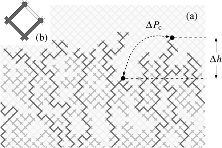
FIG. 1.: (a) The displacement pattern of a simulation on a lattice of $25\times 35$ nodes. Nonwetting fluid (dark grey and black) is injected from below and wetting fluid (light grey) flows out along the top row. In the figure, $\Delta P_{c}$ is the capillary pressure difference between a meniscus at the bottom filled dot and a meniscus at the topmost filled dot, separated a height $\Delta h$ in the direction of the displacement. The black tubes indicate strands containing no loops, where nonwetting fluid flow. The dark grey tubes connecting to the strands, are dead ends where nonwetting fluid cannot flow because of trapped wetting fluid. (b) A tube filled with wetting fluid and surrounded on both sides by nonwetting fluid is trapped.

In the literature [8, 9, 10, 11] there has been suggested slightly different scaling behavior of $w_{s}$ as function of $C_{a}$ and a general consensus has not yet been reached. However, none of them consider the evidence observed here that the displacement patterns are loopless and that nonwetting fluid only flows in strands to displace wetting fluid. As a consequence, we show that earlier proposed theories [8, 9, 10, 11] can not be used to describe drainage when loopless nonwetting strands dominate the displacements.

Before we present the numerical results and the theoretical evidence, we briefly introduce the network model. The model porous medium consists of a square lattice of cylindrical tubes oriented at $45^{\circ}$ to the longest side of the lattice [Fig. 1(a)]. Four tubes meet at each intersection where we put a node having no volume. The disorder is introduced by (1) assigning the tubes a radius $r$ chosen at random inside a defined interval or (2) moving the intersections a randomly chosen distance away from their initial positions. In (1) all tubes have equal length $d$ but different $r$. (2) results in a distorted square lattice giving the tubes different lengths. Here $r=d/2\alpha$ where $\alpha$ is the aspect ratio between the tube length and its radius.

The tubes are initially filled with a wetting fluid of viscosity $\mu_{w}$ and a nonwetting fluid of viscosity $\mu_{nw}\geq\mu_{w}$, is injected at constant injection rate $Q$ along the bottom row (inlet). The viscosity ratio $M$ is defined as $M\equiv\mu_{nw}/\mu_{w}$. The wetting fluid is displaced and flows out along the top row (outlet). There are periodic boundary conditions in the orthogonal direction. The fluids are assumed immiscible, hence an interface (a meniscus) is located where the fluids meet in the tubes. The capillary pressure $p_{c}$ of a meniscus is given by $p_{c}=(2\gamma/r)\left[1-\cos(2\pi x/d)\right]$. The first term is Young-Laplace law for a cylindrical tube when perfect wetting is assumed and in the second term $x$ is the position of the meniscus in the tube ($0\leq x\leq d$). Thus, with respect to the capillary pressure we treat the tubes as if they were hourglass shaped with effective radii following a smooth function. By letting $p_{c}$ vary as above, we include the effect of local readjustments of the menisci at pore level [6] which is important for the description of burst dynamics [12]. The detailed modeling of $p_{c}$ costs computation time, but is necessary in order to properly simulate the capillary pressure behavior along the front.

The volume flux $q_{ij}$ through a tube between the $i$th and the $j$th node is given by Washburn equation [13]: $q_{ij}=-(\sigma_{ij}k_{ij}/\mu_{ij})(p_{j}-p_{i}-p_{c,ij})/d_{ij}$. Here $k_{ij}$ is the permeability of the tube, $\sigma_{ij}$ is the average cross section of the tube, $p_{i}$ and $p_{j}$ is the pressures at node $i$ and $j$ respectively, and $p_{c,ij}$ is the sum of the capillary pressures of the menisci inside the tube. A tube partially filled with both liquids, is allowed to contain one or two menisci. Furthermore, $\mu_{ij}$ denotes the effective viscosity given by the sum of the volume fractions of each fluid inside the tube multiplied by their respective viscosities. Inserting the above equation for $q_{ij}$ into Kirchhoff equations at every node (volume flux conservation), $\sum_{j}q_{ij}=0$, constitutes a set of linear equations which are to be solved for $p_{i}$. The set of equations is solved by using the Conjugate Gradient method with the constraint that $Q$ is held fixed. See Refs. [6, 7] for details on the numerical scheme updating the menisci and solving $p_{i}$.

The front between the two phases is detected by running a Hoshen-Kopelman algorithm [14] on the lattice. The front width is defined as the standard deviation of the distances between each meniscus along the front and the average front position in the direction of the displacement. $\Delta P_{c}$ as function of $\Delta h$ is calculated by taking the mean of the capillary pressure differences between all pairs of menisci separated a height $\Delta h$ along the front. The capillary pressure difference between a pair of menisci is calculated by taking the capillary pressure of the meniscus closest to the inlet minus the capillary pressure of the meniscus closest to the outlet [Fig. 1(a)].

FIG. 2.: $\Delta P_{c}$ as function of $\Delta h$ for high and intermediate $C_{a}$ with $M=100$ on a lattice of $25\times 35$ nodes, and for low $C_{a}$ with $M=1$ on a lattice of $40\times 60$ nodes.

Figure 2 shows $\Delta P_{c}$ as function of $\Delta h$ for simulations performed at three different $C_{a}$’s with $M=100$ or $1$. The simulations with $M=100$ were performed on a $25\times 35$ nodes lattice with $\mu_{nw}=10$ P, $\mu_{w}=0.10$ P, and $\gamma=30$ dyn/cm. The disorder was introduced by choosing the tube radii at random in the interval $0.05d\leq r_{ij}\leq d$. The tube length was $d=0.1$ cm. The simulations with $M=1$ were performed on a distorted lattice of $40\times 60$ nodes where $0.02\ \mbox{cm}\leq d_{ij}\leq 0.18$ cm and $r_{ij}=d_{ij}/2\alpha$ with $\alpha=1.25$. Here $\mu_{nw}=\mu_{w}=0.5$ P. To obtain reliable average quantities we did 10–30 simulations at each $C_{a}$ with different sets of random $r_{ij}$ or $d_{ij}$.

From Fig. 2 we observe that $\Delta P_{c}$ increases roughly linearly as function of $\Delta h$. At lowest $C_{a}$ no clear stabilization of the front was observed due to the finite size of the system. At higher $C_{a}$ the viscous gradient stabilizes the front. The gradient causes the capillary pressure of the menisci closest to the inlet to exceed the capillary pressure of the menisci lying in the uppermost part. Thus, the menisci closest to the inlet will more easily penetrate a narrow tube compared to menisci further down stream. This will eventually stabilize the front.

To save computation time and thereby be able to study $\Delta P_{c}$ on larger lattices in the small $C_{a}$ regime, we have generated bond invasion percolation (IP) patterns with trapping on lattices of $200\times 300$ nodes. The IP patterns were generated on the bonds in a square lattice with the bonds oriented diagonally at $45^{\circ}$. Hence, the bonds correspond to the tubes in our network model. Each bond was assigned a random number $f_{ij}$ in the interval $[0,1]$. A small stabilizing gradient $g=0.05$ was applied, giving an occupation threshold $t_{ij}$ of every bond: $t_{ij}=f_{ij}+gh_{ij}$ [8, 15]. Here $h_{ij}$ denotes the height of the bond above the bottom row. The occupation of bonds started at the bottom row, and the next bond to be occupied was always the bond with the lowest threshold value from the set of empty bonds along the invasion front. The generated IP patterns are similar to the site-bond IP patterns in [16] and we assume they are statistical equal to structures that would have been obtained in a corresponding complete displacement simulation.

When the IP patterns became well developed with trapped (wetting) clusters of sizes between the bond length and the front width, the tubes in our network model were filled with nonwetting and wetting fluid according to occupied and empty bonds in the IP lattice. Moreover, the radii $r_{ij}$ of the tubes were mapped to the random numbers $f_{ij}$ of the bonds as $r_{ij}=[0.05+0.95(1-f_{ij})]d$. Thus, $0.05d\leq r_{ij}\leq d$ and we set the tube length $d=0.1\,\mbox{cm}$. Note that $r_{ij}$ is mapped to $1-f_{ij}$ because in our IP algorithm the next bond to be invaded is the one with the lowest threshold value, opposite to the network model, where the widest tube will be invaded first.

After the initiation of the tube network was completed, the network model was started and the simulations were run a limited number of time steps before it was stopped. The number of time steps where chosen sufficiently large to let the menisci along the front adjust according to the viscous pressure set up by the injection rate.

Totally, we generated four IP patterns with different sets of $f_{ij}$ and every pattern was loaded into the network model. The result of the calculated $\Delta P_{c}$ versus $\Delta h$ is shown in Fig. 3 for $C_{a}=\mbox{$9.5\!\times\!10^{-5}$}$ and $M=100$. If we assume a power law $\Delta P_{c}\propto\Delta h^{\kappa}$, we find $\kappa=1.0\pm 0.1$. The slope of the straight line in Fig. 3 is 1.0. We have also calculated $\Delta P_{c}$ for $C_{a}=\mbox{$2\!\times\!10^{-6}$}$ with $M=1$ and $M=100$ by using one of the generated IP patterns. The result of those simulations is consistent with Fig. 3.

FIG. 3.: $\log_{10}(\Delta P_{c})$ as function of $\log_{10}(\Delta h)$ for drainage simulations initiated on IP patterns at $C_{a}=\mbox{$9.5\!\times\!10^{-5}$}$ and $M=100$. The result is averaged over four different runs and the error bars denote the standard error in the mean. The slope of the solid line is 1.0.

Wilkinson [8] was the first to use percolation theory to deduce a power law between $w_{s}$ and $C_{a}$ when only viscous forces stabilize the front. In 3D, where trapping of wetting fluid is assumed to be of little importance, he suggested $w_{s}\propto{C_{a}}^{-\alpha}$ and $\alpha=\nu/(1+t-\beta+\nu)$. Here $t$ is the conductivity exponent and $\beta$ is the order parameter exponent in percolation. Blunt et al. [10] used a similar approach, however, they found $\alpha=\nu/(1+t+\nu)$ in 3D. This is identical to the result of Lenormand [9] discussing limits of fractal patterns between capillary fingering and stable displacement in 2D porous media. Blunt et al. also deduced a scaling relation for the pressure drop $\Delta P_{nw}$ across a height difference $\Delta h$ in the nonwetting phase of the front and found $\Delta P_{nw}\propto\Delta h^{t/\nu+1}$. Later on, Xu et al. [11] used the arguments of Gouyet et al. [17] and Wilkinson [8] to show that $\Delta P_{nw}\propto{\Delta h}^{t/\nu+d_{\text{E}}-1-\beta/\nu}$, where $d_{\text{E}}$ is the Euclidean dimension of the space in which the front is embedded. They also argued that $\Delta P_{c}=\Delta P_{nw}-\Delta P_{w}$ where $\Delta P_{w}$ denoting the pressure drop in the wetting phase of the front, is linearly dependent on $\Delta h$ due to the compact displaced fluid [see Fig. 1(a)]. Thus, the result of Xu et al. would in 2D predict $\Delta P_{c}\propto\Delta h^{1.9}$ where we have used $t=1.3$, $\nu=4/3$, $\beta=5/36$, and $d_{\text{E}}=2$. Our simulations give $\Delta P_{c}\propto\Delta h^{\kappa}$ and $\kappa=1.0\pm 0.1$. Below we present an alternative view on the displacement pattern from those first suggested by Wilkinson. The alternative view is based upon the loopless nonwetting strands and is supported by our numerical result.

The simulated displacement patterns show that the nonwetting fluid contains no closed loops [Fig. 1(a)] because wetting fluid may be trapped in single tubes, due to volume conservation [Fig. 1(b)]. Because of fluid trapping in single tubes, the invading fluid flows in separate strands that cannot coalesce. We note that the definition in in Fig. 1(b) can be easily generalized to 3D [18], since increasing the coordination number of the lattice does not change the trapping rule. Therefore, we expect loopless patterns to develop in 3D lattices and our arguments that we present below should apply there too. We also note that trapping of wetting fluid is more difficult in real porous media due to a more complex topology of pores and throats there. Loopless IP patterns have earlier been observed in Refs. [16, 19, 20].

From Fig. 1(a) we may separate the displacement pattern into two parts: one consisting of the frontal region continuously covering new tubes, and the other consisting of the more static structure behind the front. The frontal region is supplied by nonwetting fluid through strands connecting the frontal region to the inlet. When the strands approach the frontal region they are more likely to split. Since we are dealing with a square lattice, a splitting strand may create either two or three new strands. As the strands proceed further into the frontal region they split again and again and eventually they cover the frontal region completely [see Fig. 1(a)].

On IP patterns without loops [16, 18, 20] the length $l$ of the minimum path between two points separated an Euclidean distance $R$ scales like $l\propto R^{D_{s}}$ where $D_{s}$ is the fractal dimension of the shortest path. We assume that the displacement pattern of the frontal region for length less than the correlation length (in our case $w_{s}$) is statistically equal to IP patterns in [16]. Therefore, the length of a strand in the frontal region is proportional to $\Delta h^{D_{s}}$ when $\Delta h$ is less than $w_{s}$. If we assume that on the average every tube in the lattice has same mobility ($k_{ij}/\mu_{ij}$), this causes the fluid pressure within a single strand to drop like $\Delta h^{D_{s}}$ as long as the strand does not split. When the strand splits volume conservation causes the volume fluxes through the new strands to be less than the flux in the strand before it splits. Hence, following a path where strands split will cause the pressure to drop as $\Delta h^{\kappa}$ where $\kappa\leq D_{s}$.

From the above arguments we conclude that the pressure drop $\Delta P_{nw}$, in the nonwetting phase of the frontal region (that is the strands) should scale as $\Delta P_{nw}\propto\Delta h^{\kappa}$ where $\kappa\leq D_{s}$. In 2D two different values for $D_{s}$ have been reported: $D_{s}=1.22$ [18, 20] and $D_{s}=1.14$ [16]. Both values are consistent with our simulations finding $\kappa=1.0\pm 0.1$.

The evidence that $\kappa\simeq 1.0$ may influence the scaling of $w_{s}$ as function of $C_{a}$. At low $C_{a}$ simulations show that $\Delta\widehat{P}_{c}\propto C_{a}\Delta h^{1.0}$ [21]. Here $\Delta\widehat{P}_{c}$ denotes the capillary pressure difference when the front is stationary. That means, $\Delta\widehat{P}_{c}$ excludes situations where nonwetting fluid rapidly invades new tubes due to local instabilities. At sufficiently low $C_{a}$ the displacement can be mapped to percolation giving $\Delta\widehat{P}_{c}\propto f-f_{c}\propto\xi^{-1/\nu}$ [8, 15, 17]. Here $f$ is the occupation probability of the bonds, $f_{c}$ is the percolation threshold, and $\xi\propto w_{s}$ is the correlation length. By combining the above relations, we obtain $w_{s}\propto{C_{a}}^{-\alpha}$ where $\alpha=\nu/(1+\nu\kappa)$. In 2D $\nu=4/3$ and inserting $\kappa=1.0$ gives $\alpha\approx 0.57$. At high $C_{a}$ we expect a crossover to another type of behavior since it is not clear if the mapping to percolation [8, 15, 17] is valid there. We note that Wilkinson’s result [8] gives $\alpha\approx 0.38$ in 2D.

In summary we conclude that $\Delta P_{c}\propto\Delta h^{\kappa}$ where our simulations gives $\kappa=1.0\pm 0.1$. By describing the displacement structure in terms of loopless strands [16, 20] we have argued that $\kappa\leq D_{s}$, where $D_{s}$ is the fractal dimension of the shortest path between two points on IP patterns without loops. In 2D two values of $D_{s}$ has been reported ($1.14$ [16] and $1.22$ [18, 20]) and both are consistent with our numerical result $\kappa\simeq 1.0$. We conclude that earlier suggested theories [8, 9, 10, 11] are not compatible in situations where a loopless pattern with nonwetting strands dominate the displacement. We have also shown that $\alpha$ in $w_{s}\propto{C_{a}}^{-\alpha}$, may be influenced by the evidence that $\kappa\leq D_{s}$. Work is in progress to investigate our arguments in 3D and the effect of loops on $\kappa$.

The authors thank J. Feder and E. G. Flekkøy for valuable comments. The work is supported by the Norwegian Research Council (NFR) through a “SUP” program and we acknowledge them for a grant of computer time.

REFERENCES

- [1] K. J. Måløy, J. Feder, and T. Jøssang, Phys. Rev. Lett. 55, 2688 (1985). J.-D. Chen and D. Wilkinson, Phys. Rev. Lett. 55, 1892 (1985).
- [2] R. Lenormand, E. Touboul, and C. Zarcone, J. Fluid Mech. 189, 165 (1988).
- [3] M. Cieplak and M. O. Robbins, Phys. Rev. Lett. 60, 2042 (1988).
- [4] P. G. de Gennes and E. Guyon, J. Mec. (Paris) 17, 403 (1978). R. Chandler, J. Koplik, K. Lerman, and J. F. Willemsen, J. Fluid Mech. 119, 249 (1982). D. Wilkinson and J. F. Willemsen, J. Phys. A 16, 3365 (1983). R. Lenormand and C. Zarcone, Phys. Rev. Lett. 54, 2226 (1985).
- [5] O. I. Frette, K. J. Måløy, J. Schmittbuhl, and A. Hansen, Phys. Rev. E. 55, 2969 (1997).
- [6] E. Aker, K. J. Måløy, A. Hansen, and G. G. Batrouni, Transp. Porous Media 32, 163 (1998).
- [7] E. Aker, K. J. Måløy, and A. Hansen, Phys. Rev. E 58, 2217 (1998).
- [8] D. Wilkinson, Phys. Rev. A 34, 1380 (1986).
- [9] R. Lenormand, Proc. R. Soc. London, Ser. A 423, 159 (1989).
- [10] M. Blunt, M. J. King, and H. Scher, Phys. Rev. A 46, 7680 (1992).
- [11] B. Xu, Y. C. Yortsos, and D. Salin, Phys. Rev. E 57, 739 (1998).
- [12] W. B. Haines, J. Agric. Sci. 20, 97 (1930). L. Furuberg, K. J. Måløy, and J. Feder, Phys. Rev. E 53, 966 (1996).
- [13] E. W. Washburn, Phys. Rev. 17, 273 (1921).
- [14] D. Stauffer and A. Aharony. Introduction to Percolation Theory. (Taylor & Francis, London, 1992).
- [15] A. Birovljev, L. Furuberg, J. Feder, T. Jøssang, K. J. Måløy, and A. Aharony, Phys. Rev. Lett. 67, 584 (1991).
- [16] M. Sahimi, M. Hashemi, and J. Ghassemzadeh, Physica A 260, 231 (1998).
- [17] J.-F. Gouyet, M. Rosso, and B. Sapoval, Phys. Rev. B 37, 1832 (1988).
- [18] M. Porto, S. Havlin, S. Schwarzer, and A. Bunde, Phys. Rev. Lett. 79, 4060 (1997).
- [19] H. Kharabaf and Y. C. Yortsos, Phys. Rev. E 55, 7177 (1997).
- [20] M. Cieplak, A. Maritan, and J. R. Banavar, Phys. Rev. Lett. 76, 3754 (1996).
- [21] E. Aker, K. J. Måløy, and A. Hansen, In press Phys. Rev. E 61 (2000).