Strong Coupling Theory of Two Level Atoms in Periodic Fields

Abstract

We present a new convergent strong coupling expansion for two-level atoms in external periodic fields, free of secular terms. As a first application, we show that the coherent destruction of tunnelling is a third-order effect. We also present an exact treatment of the high-frequency region, and compare it with the theory of averaging. The qualitative frequency spectrum of the transition probability amplitude contains an effective Rabi frequency.

The advent of strong laser pulses has stimulated interest in strong-coupling expansions in quantum optics and quantum electrodynamics. Such expansions are also of considerable general conceptual interest in several branches of physics. However, particularly in the case of periodic and quasi-periodic perturbations, the usual series, e.g., the Dyson series, are plagued by secular terms, leading to a violation of unitarity when the expansion is truncated at any order. In addition, small denominators appear in the quasi-periodic case (see the discussion in the introduction in [1]). These problems have been formally solved in a nice letter by W. Scherer [2] and in the papers which followed [3, 4]. The main shortcoming in these works is that convergence was not controlled, an admittedly difficult enterprise. By writing an Ansatz in exponential form, and “renormalizing” the exponential inductively, we were able to eliminate completely the secular terms and to prove convergence in the special case of a two-level atom subject to a periodic perturbation, described by the Hamiltonian [5]

$$H_{1}(t)\;=\;\epsilon\sigma_{3}-f(t)\sigma_{1}.$$ (1)

The corresponding Schrödinger equation is

$$i\partial_{t}\Psi(t)\;=\;H_{1}(t)\Psi(t),$$ (2)

adopting $\hbar=1$ for simplicity. Above $f(t)$ is of the form

$$f(t)\;=\;\sum_{n\in{\mathbb{Z}}}F_{n}e^{in\omega t},$$ (3)

with $\overline{F_{n}}=F_{-n}$, since $f$ is real, and $\sigma_{i}$ are the Pauli matrices satisfying $[\sigma_{1},\;\sigma_{2}]=2i\sigma_{3}$ plus cyclic permutations. Assuming $F_{n}$ of order one, the situation where $\epsilon$ is “small” characterizes the strong coupling domain.

It is convenient to perform a time-independent unitary rotation of $\pi/2$ around the 2-axis in (1), replacing $H_{1}(t)$ by

$$H_{2}(t)\;=\;\epsilon\sigma_{1}+f(t)\sigma_{3}$$ (4)

and the Schrödinger equation by

$$i\partial_{t}\Phi(t)\;=\;H_{2}(t)\Phi(t),$$ (5)

with $\Phi(t)=\exp(-i\pi\sigma_{2}/4)\Psi(t)$.

The following result was proved in [1]. Let $f$ be continuously differentiable and $g$ be a particular solution of the generalized Riccati equation

$$g^{\prime}-ig^{2}-2ifg+i\epsilon^{2}\;=\;0.$$ (6)

Then the function $\Phi:{{\mathbb{R}}}\to{{\mathbb{C}}}^{2}$ given by

$$\Phi(t)\;=\;\left(\begin{array}[]{c}\phi_{+}(t)\\ \phi_{-}(t)\end{array}\right)\;=\;U(t)\Phi(0),$$ (7)

where

$$U(t)\equiv\left(\begin{array}[]{cc}R(t)(1+ig_{0}S(t))&-i\epsilon R(t)S(t)\\ &\\ -i\epsilon\overline{R(t)}\overline{S(t)}&\overline{R(t)}(1-i\overline{g_{0}}\overline{S(t)})\end{array}\right),$$ (8)

with $g_{0}\equiv g(0)$,

$$R(t)\;\equiv\;\exp\left(-i\int_{0}^{t}(f(\tau)+g(\tau))\,d\tau\right)$$ (9)

and $S(t)\equiv\int_{0}^{t}R(\tau)^{-2}\,d\tau$, is a solution of the Schrödinger equation (5) with initial value $\Phi(0)=\left(\begin{array}[]{c}\phi_{+}(0)\\ \phi_{-}(0)\end{array}\right)$. A simple computation [1] shows that the components $\phi_{\pm}$ of $\Phi(t)$ satisfy a complex version of Hill’s equation

$$\phi{{}_{\pm}}^{\prime\prime}+(\pm if^{\prime}+\epsilon^{2}+f^{2})\phi_{\pm}\;=\;0.$$ (10)

In [1] we attempted to solve (10) using the Ansatz $\phi(t)=\exp\left(-i\int_{0}^{t}(f(\tau)+g(\tau))d\tau\right)$, from which it follows that $g$ has to satisfy the generalized Riccati equation (6). A similar idea was used by F. Bloch and A. Siegert in [6]. For $\epsilon\equiv 0$ a solution of (6) is given by $\exp\left(-i\int_{0}^{t}f(\tau)d\tau\right)$. Thus, in the above Ansatz we are searching for solutions in terms of an “effective external field” of the form $f+g$, with $g$ vanishing for $\epsilon=0$. It is thus natural to pose

$$g(t)\;=\;\sum_{n=1}^{\infty}\epsilon^{n}G^{(n)}(t),$$ (11)

where

$$G^{(n)}(t)\;\equiv\;q(t)c_{n}(t)$$ (12)

and

$$q(t)\;\equiv\;\exp\left(i\int_{0}^{t}f(\tau)d\tau\right).$$ (13)

Inserting (11)-(12) into (6) yields a sequence of recursive equations for the coefficients $c_{n}$, whose solutions are

$$c_{1}(t) = \alpha_{1}\,q(t),$$ (14)

$$c_{2}(t) = q(t)\,\left[i\int_{0}^{t}\left(\alpha_{1}^{2}q(\tau)^{2}-q(\tau)^{-2}\right)d\tau+\alpha_{2}\right],$$ (15)

$$c_{n}(t) = q(t)\,\left[i\left(\int_{0}^{t}\sum_{p=1}^{n-1}c_{p}(\tau)c_{n-p}(\tau)\,d\tau\right)+\alpha_{n}\right],$$ (16)

for $n\geq 3$, where the $\alpha_{n}$ are arbitrary integration constants. The main point is that these constants may be chosen inductively in order to cancel the secular terms. For instance, in order to cancel the secular term in $c_{2}$ in (15), the integrand cannot contain a constant term, which equals the mean-value term

$$M(q^{2})\;\equiv\;\lim_{T\to\infty}\frac{1}{2T}\int_{-T}^{T}q^{2}(\tau)\,d\tau\;\neq\;0.$$ (17)

Then it follows from (15) that one must require

$$M(\alpha_{1}^{2}q^{2}-q^{-2})\;=\;0\;\Longrightarrow\;\alpha_{1}^{2}\;=\;\frac{\overline{M(q^{2})}}{M(q^{2})}.$$ (18)

It was proved in [1] that one may proceed in this way and establish the absence of secular terms of any order. Similar results are valid if (17) is not satisfied.

In the quasi-periodic case we were not able to show convergence in (11), and, in fact, it is not expected [1]. Hence, (11) is to be viewed as a formal power series. In the periodic case (3) much stronger results are possible, as we now discuss.

Let $G_{m}^{(n)}$, $C_{m}^{(n)}$, $Q_{m}$ and $Q_{m}^{(2)}$ denote the Fourier coefficients of $G^{(n)}(t)$, $c_{n}(t)$ (given in (11)-(12)), $q(t)$ (given in (13)) and $q^{2}(t)$, respectively, defined as in (3). Due to the multiplication by $q(t)$ in (12) the $G_{m}^{(n)}$ are given by convolutions

$$G_{m}^{(n)}\;=\;\sum_{l=-\infty}^{\infty}Q_{m-l}C_{l}^{(n)}.$$ (19)

The $C_{l}^{(n)}$, the Fourier components of $c_{n}(t)$, have, by (14)-(16), explicit expressions in terms of the $Q_{m}$ and $Q_{m}^{(2)}$, for instance, if (17) holds and $\alpha_{1}$ is given by (18),

$$C_{m}^{(1)} = \alpha_{1}Q_{m},$$ (20)

$$C_{m}^{(2)} = \sum_{n=\infty\atop n\neq 0}^{\infty}\frac{\left(\alpha_{1}^{2}Q^{(2)}_{n}-\overline{Q^{(2)}_{-n}}\right)}{n\omega}\left[Q_{m-n}-\frac{Q_{m}Q_{-n}^{(2)}}{Q_{0}^{(2)}}\right],$$ (21)

Note that, above, $Q_{0}^{(2)}=M(q^{2})\neq 0$. The solution for the case $M(q^{2})=0$ is found in [1, 7]. Finally, let

$$\Omega\;=\;\Omega(\epsilon)\;\equiv\;F_{0}+G_{0}(\epsilon),$$ (22)

$$H_{n}\equiv\left\{\begin{array}[]{cl}[F_{n}+G_{n}(\epsilon)](n\omega)^{-1},&\mbox{for }n\neq 0\\ &\\ 0,&\mbox{for }n=0\end{array}\right.,$$ (23)

and $\displaystyle\gamma_{f}(\epsilon)\equiv i\sum_{m\in{\mathbb{Z}}}\,H_{m}$, with $\displaystyle G_{m}(\epsilon)\equiv\sum_{n=1}^{\infty}G_{m}^{(n)}\epsilon^{n}$. Then $R(t)$, in (9), is given by

$$R(t)\;=\;e^{-i\gamma_{f}(\epsilon)}\;e^{-i\Omega t}\;{\cal R}(\infty,\;t),$$ (24)

with $\displaystyle{\cal R}(N,\;t)\equiv\exp\left(-\sum_{n=-N}^{N}H_{n}e^{in\omega t}\right)$. By (8), the complete wave function is known once (24) is given; (8) and (24) also show that the wave-function is of the Floquet form, with secular frequencies $\pm\Omega$.

In reference [7] we have proven the following result: for $f$ periodic the $\epsilon$-expansion (11) has a nonzero radius of convergence. Our estimate for this radius is not optimal and we refrain from quoting it here, but we remark that the expansion does converge for high frequencies, i.e., $\omega\gg\epsilon$, a condition that we assume in the following.

We now consider in (3) the special case

$$F_{n}\;=\;\frac{1}{2}(\delta_{n,\;1}+\delta_{n,\;-1}),$$ (25)

corresponding to $f(t)=\cos(\omega t)$. For this case

$$Q_{m}\;=\;J_{m}\left(\frac{1}{\omega}\right)\;\mbox{ and }\;Q_{m}^{(2)}\;=\;J_{m}\left(\frac{2}{\omega}\right).$$ (26)

By (18), $\alpha_{1}=1$.

The transition amplitude $A_{21}$ from the lowest energy atomic state $\left({0\atop 1}\right)$ of (1) to the upper level $\left({1\atop 0}\right)$ is

$$A_{21}(t)\;=\;\left(\psi_{1},\;U(t)\psi_{2}\right),$$ (27)

where $U(t)$ is given by (8) and $\psi_{2}=\frac{1}{\sqrt{2}}\left({1\atop-1}\right)$, $\psi_{1}=\frac{1}{\sqrt{2}}\left({1\atop 1}\right)$ are the corresponding eigenstates of the rotated Hamiltonian $H_{2}$, given by (4). The tunnelling amplitude corresponds to the transition probability

$$\tilde{A}_{21}(t)\;=\;\left(\tilde{\psi}_{1},\;U(t)\tilde{\psi}_{2}\right),$$ (28)

where $\tilde{\psi}_{2}=\left({0\atop 1}\right)$, $\tilde{\psi}_{1}=\left({1\atop 0}\right)$. The latter represent the localized states (eigenstates of the field term, proportional to $\sigma_{3}$, in (4)), and $\tilde{A}_{21}=0$ means absence of tunnelling between these states. Indeed, (4) is a semi-classical approximation to the spin-Boson system treated in [8]. In the full quantized case, considered in [8], $\tilde{\psi}_{1}$ and $\tilde{\psi}_{2}$ differ macroscopically because they are dressed by photon clouds, and for $\epsilon$ sufficiently small there is always localization, i.e., no tunnelling. This is not the case here, as we shall see.

Fig. 1 shows the exact result for $|A_{21}(t)|^{2}$ to fifth order in $\epsilon$ for about $12$ cycles of $\omega$. We see clearly the domination of the external frequency $\omega$, in agreement with the theory of averaging. Eq. (5) may be transformed to

$$\partial_{t}\tilde{\psi}\;=\;\epsilon f(t,\;\tilde{\psi})$$ (29)

with $\tilde{\psi}=\exp\left(i\int_{0}^{t}f(\tau)d\tau\right)\psi$, and

$$f(t,\;\tilde{\psi})\;=\;\left(\begin{array}[]{cc}0&e^{2i\sin(\omega t)/\omega}\\ e^{-2i\sin(\omega t)/\omega}&0\end{array}\right)\tilde{\psi}.$$ (30)

By (29) and (30), the averaged equation $\partial_{t}\tilde{\psi_{0}}=\epsilon f^{(0)}(\tilde{\psi_{0}})$ with $f^{(0)}(\tilde{\psi_{0}})=\frac{1}{T}\int_{0}^{T}f(t,\,\tilde{\psi_{0}})$ and $T=2\pi/\omega$, is

$$i\partial_{t}\tilde{\psi_{0}}\;=\;\epsilon J_{0}\left(\frac{2}{\omega}\right)\sigma_{1}\tilde{\psi_{0}}$$ (31)

and a well known theorem [9] yields $\left|\tilde{\psi}(t)-\tilde{\psi_{0}}(t)\right|=O(\epsilon/\omega)$ on the time scale $1/\epsilon$. Hence $A_{21}$ is close to

$$\left(\psi_{1},\;\exp\left(-i\epsilon J_{0}\left(\frac{2}{\omega}\right)\sigma_{1}t\right)\exp\left(i\frac{\sin(\omega t)}{\omega}\sigma_{3}\right)\psi_{2}\right)\;=\;$$

$$i\exp\left(-i\epsilon J_{0}\left(\frac{2}{\omega}\right)t\right)\sin\left(\frac{\sin(\omega t)}{\omega}\right).$$

Since $\displaystyle\sin\left(\frac{\sin(\omega t)}{\omega}\right)=2\sum_{k=0}^{\infty}J_{2k+1}\left(\frac{1}{\omega}\right)\sin\left[(2k+1)\omega t\right]$, we see that in this case the spectrum is dominated by the harmonics of the frequency $\omega$ of the external field, in agreement with Fig. 1. Notice, however, that, while averaging is applicable to times up to $O(1/\epsilon)$, the exact theory is applicable to all times. Applying the averaging theory to $\tilde{A}_{21}$, we are led to the matrix element

$$\left(\exp\left(i\frac{\sin(\omega t)}{\omega}\sigma_{3}\right)\tilde{\psi}_{1},\;\exp\left(-i\epsilon J_{0}\left(\chi\right)\sigma_{1}t\right)\tilde{\psi}_{2}\right)=$$

$$-ie^{i\frac{\sin(\omega t)}{\omega}}\sin\left(\epsilon J_{0}\left(\chi\right)t\right)\,\simeq\,-iJ_{0}\left(\frac{\chi}{2}\right)\sin\left(\epsilon J_{0}\left(\chi\right)t\right),$$

with $\chi\equiv 2/\omega$. This result agrees with (24) and Fig. 2, which shows the exact result for $|\tilde{A}_{21}(t)|^{2}$ to fifth order in $\epsilon$ for $t$ from $0$ to $2\pi/\Omega$. Fig. 2 shows that $\Omega(\epsilon)$, the secular frequency given by (22), dominates in this case. There, $\Omega(\epsilon)\simeq 7.6\,10^{-3}$ for the values of $\epsilon$ and $\omega$ chosen.

Notice that by (19), (20), (22) and (26) $\Omega(\epsilon)\simeq\epsilon J_{0}(\chi)$, to first order in $\epsilon$. Thus, the first order contribution approaches zero if $\chi$ approaches one of the zeros of the Bessel function $J_{0}$. The second order contribution to $\Omega$ is $\displaystyle\epsilon^{2}\sum_{l\in{\mathbb{Z}}}Q_{-l}C_{l}^{(2)}$, and is identically zero, as one sees using (21). The third order contribution to $\Omega$ is

$$-\frac{2\epsilon^{3}}{\omega^{2}}\sum_{n_{1},\;n_{2}=-\infty}^{\infty}\frac{J_{2n_{1}+1}(\chi)J_{2n_{2}+1}(\chi)J_{-2(n_{1}+n_{2}+1)}(\chi)}{(2n_{1}+1)(2n_{2}+1)}$$

and is non-zero if $\chi$ coincides with one of the zeros of $J_{0}$. Hence, when $2/\omega$ approaches one of the zeros of the Bessel function $J_{0}$ the lowest non-vanishing contribution to $\Omega$ is of third order in $\epsilon$ and, hence, rather small. This means that for such values of $\omega$ the tunnelling is very heavily, although not exactly, suppressed.

Hampering and destruction of tunnelling have been studied in [10, 11] for particles, and in [12, 13] for spins. The latter use the method of averaging, but we emphasize that in the case treated above, $\omega\gg\epsilon$ is satisfied for $\epsilon$ sufficiently small, and thus the result is exact, i.e., valid for all times. In addition, the features regarding the order of the expansion are new.

At resonance $\omega=2\epsilon$ we are not able to prove that the expansion converges. It is, nevertheless, a well-defined formal expansion, in contrast to strong-coupling approximations of Keldish type, which are beset with difficulties (see, e.g. [14] and references given there). Moreover, as we shall show, it includes interesting effects of dressing of the atoms by the photon field (in the semi-classical approximation) which yields the external field Floquet description, rigorously justified in [15]. Such effects appear in the rotating-wave-approximation (RWA) in the form of a Rabi frequency (see, e.g. [15]), but the present model is not close to RWA, since the rotating and counter-rotating terms in (1) are of the same order of magnitude. Moreover, the RWA is not justified for large coupling, but the solution of (5) might have some similarity to the solution obtained when the RWA is performed. If so, the effective frequency of oscillation of $A_{21}$ would not differ much from the Rabi frequency (see [15])

$$\Omega_{R}\;=\;\left[(\omega-2\epsilon)^{2}+4\right]^{1/2}\simeq 2$$ (32)

for $\omega\simeq 2\epsilon$ (or, in general, for $\omega=O(\epsilon)$ and $\epsilon$ small). Indeed, $\Omega_{R}$ makes its appearance in (24) in a most interesting way: by (19)-(20)-(23) and (26), $H_{n}$ in ${\cal R}(\infty,\,t)$ equals, to first order in $\epsilon$,

$$\frac{F_{n}}{n\omega}+\epsilon\frac{J_{n}\left(\frac{2}{\omega}\right)}{n\omega},$$ (33)

with $F_{n}$ given by (25). The greatest contributions of (33) arises for small $n$ (due to the factor $n^{-1}$) and when the argument of the Bessel function equals its order, i.e., $n=2/\omega$, and the corresponding frequency in (24) is $n\omega=\frac{2}{\omega}\omega=2$, which compares well with (32). In Fig. 3 we show this last effect for ${\cal R}(N,\;t)$. We considered the quantity ${\cal E}(N,\;t)\equiv\left|\frac{{\cal R}(N,\;t)}{{\cal R}(\infty,\;t)}-1\right|$ which measures the error made by including in (24) only the first $N$ terms of the sum involving $H_{n}$ in ${\cal R}(\infty,\;t)$. In Fig. 3 we considered the resonant case with $\omega=2\epsilon=2\,10^{-2}$ and $t=0.7\pi/\Omega$. The qualitative behaviour is the same for other values of $t$. We see from Fig. 3 that mainly only small $n$ and $n$ around $2/\omega$ contribute. The effect of adding in the second order contribution is negligible for the range of values of $\epsilon$ considered.

In conclusion, the new strong-coupling expansion allows considerable insight into both the high-frequency and resonance regimes, and yields an interesting unexpected result for the coherent destruction of tunnelling.

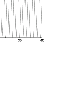
FIG. 1.: The amplitude $|A_{21}(t)|^{2}$. Here $\epsilon=0.01$ and $\omega=2$.

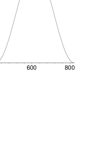
FIG. 2.: The amplitude $|\tilde{A}_{21}(t)|^{2}$. Here $\epsilon=0.01$ and $\omega=2$.

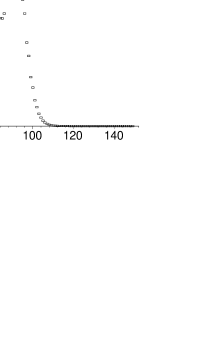
FIG. 3.: The quantity ${\cal E}(N,\;t)$ as a function of $N$.

REFERENCES

[1] J. C. A. Barata. “On Formal Quasi-Periodic Solutions of
the Schrödinger Equation for a Two-Level System with a Hamiltonian
Depending Quasi-Periodically on Time”. mp_arc 98-252. To appear in
Rev. Math. Phys.
[2] W. Scherer. Phys. Rev. Lett. 74, 1495 (1995).
[3] W. Scherer. J. Phys. A30, 2825 (1997).
[4] W. Scherer. J. Phys. A27, 8231 (1994).
[5] S. H. Autler and C. H. Townes. Phys. Rev. 100, 703-722 (1955).
[6] F. Bloch and A. Siegert. Phys. Rev. 57,
522-527 (1940).
[7] J. C. A. Barata. “Convergent Perturbative Solutions of
the Schrödinger Equation for a Two-Level System with a Hamiltonian
Depending Periodically on Time”. math-ph/9903041. Submitted to
Commun. Math. Phys.
[8] H. Spohn and R. Dümcke. J. Stat. Phys. 41, 389 (1985).
[9] F. Verhulst. “Nonlinear Differential Equations and
Dynamical Systems”. Springer (1990). Theorem 11.1.
[10] F. Grossman, T. Dittrich, P.
Jung, P. Hänggi. Phys. Rev. Lett. 67, 516-519 (1991).
[11] Y. Kayanuma. Phys. Rev. A 50, 843-845
(1994).
[12] J. L. van Hemmen and
A. Sütő. J. Phys. Condens. Matter 9, 208 (1997).
[13] J. L. van Hemmen and
W. F. Wreszinski. Phys. Rev. B57, 1007 (1998).
[14] W. Becker, L. Davidovich and J. K. McIver. Phys. Rev.
A49, 1131 (1994).
[15] S. Guérin, F. Monti, J.-M. Dupont and H. R. Jauslin.
J. Phys. A30, 7193 (1997).