Search for exchange-antisymmetric two-photon states

Abstract

Atomic two-photon J=0 $\leftrightarrow$J’=1 transitions are forbidden for photons of the same energy. This selection rule is related to the fact that photons obey Bose-Einstein statistics. We have searched for small violations of this selection rule by studying transitions in atomic Ba. We set a limit on the probability $v$ that photons are in exchange-antisymmetric states: $v<1.2\cdot 10^{-7}$.

Recent experiments have explored the possibility of small violations of the usual relationship between spin and statistics [3, 4, 5, 6, 7]. Although such violations are impossible within conventional quantum field theory [8], there are motivations for considering them; see e.g. Ref. [9]. If photons do not obey Bose-Einstein (BE) statistics, there will be a non-zero probability that two photons are in an exchange-antisymmetric state. Here we report the results of a search for such states based on a selection rule [10, 11] that forbids two-photon transitions between atomic states with $J=0$ and $J^{\prime}=1$ for degenerate photons (i.e., photons of equal energy).

Consider the general amplitude for a $J=0\rightarrow{}J^{\prime}=1$ two-photon transition. This amplitude is a scalar which must be constructed from the polarization vectors $\mathbf{e}_{1,2}$ of the photons and the polarization vector $\mathbf{e}_{v}$ describing the $J^{\prime}=1$ state (each exactly once); and may also contain arbitrary powers of the photon propagation directions $\hat{\mathbf{k}}_{1,2}$, and some function of the photon energies $\hbar\Omega_{1,2}$. In the specific case of E1-E1 transitions, the amplitude must be independent of $\hat{\mathbf{k}}_{1,2}$, and only one form is possible:

$$A\;\propto\;\{{\left(\mathbf{e_{1}}\mathnormal{\times}\mathbf{e_{2}}\right)}\mathnormal{\cdot}\mathbf{e_{v}}\}\>\mathnormal{F}{\left(\Omega_{1},\Omega_{2}\right)},$$ (1)

which requires orthogonally-polarized photons. If photons obey BE statistics, this amplitude must be invariant under exchange of labels $1\leftrightarrow 2$. Eqn. (1) satisfies this condition only if $\mathnormal{F}{\left(\Omega_{1},\Omega_{2}\right)}$ is odd under exchange. Therefore the amplitude must vanish in the degenerate case, if photons behave as normally expected. This argument can be readily generalized beyond the E1-E1 case [12]. For the case of counterpropagating degenerate photons (with $\mathbf{k_{2}}=-\mathbf{k_{1}}$), the Landau-Yang theorem states that all possible amplitudes vanish [13]. We consider only the E1-E1 amplitude of Eqn. (1), since higher multipolarity transitions are too weak to be observed in the present experiment.

For ordinary photons, the atomic two-photon-resonant transition rate is [10]:

$$W_{gf}{\left(\Omega_{1},\Omega_{2}\right)}\propto$$ (2)

$$|{\mathbf{e_{1a}}\mathbf{e_{2b}}}\langle{}f|Q_{ab}|g\rangle|^{2}\frac{dI_{1}}{d\Omega_{1}}\frac{dI_{2}}{d\Omega_{2}}\delta{\left(\omega_{fg}-\Omega_{1}-\Omega_{2}\right)},$$ (3)

$$Q_{ab}{\left(\Omega_{1},\Omega_{2}\right)}=$$ (4)

$$d_{a}{\left(\sum_{n}\frac{|n\rangle\langle{}n|}{\omega_{ng}-\Omega_{1}}\right)}d_{b}+d_{b}{\left(\sum_{n}\frac{|n\rangle\langle{}n|}{\omega_{ng}-\Omega_{2}}\right)}d_{a}.$$ (5)

Here indices $g$, $f$, and $n$ indicate ground, final, and (virtual) intermediate states of the transition; $\frac{dI_{1(2)}}{d\Omega_{1(2)}}$ are the spectral distributions of light intensity; $\omega_{ij}$ are frequencies of atomic transitions; $\mathbf{d}$ is the dipole operator; and the subscripts $a,b$ refer to Cartesian components. Consistent with our experimental conditions, we neglect Doppler and natural widths compared to laser spectral widths. For a $J=0\rightarrow{}J^{\prime}=1$ transition, only the irreducible rank-1 component of $Q_{ab}$ can contribute to the matrix element [10, 11]. Thus

$$Q_{ab}{\left(\Omega_{1},\Omega_{2}\right)}=Q_{ab}^{(1)}=\frac{1}{2}{\left(Q_{ab}-Q_{ba}\right)}=$$ (6)

$$\frac{1}{2}{\left(\Omega_{1}-\Omega_{2}\right)}\sum_{n}\frac{{\left\{d_{a}|n\rangle\langle{}n|d_{b}-d_{b}|n\rangle\langle{}n|d_{a}\right\}}}{{\left(\omega_{ng}-\Omega_{1}\right)}{\left(\omega_{ng}-\Omega_{2}\right)}}.$$ (7)

Eqn. (7) shows explicitly that degenerate transitions are forbidden: $Q_{ab}{\left(\Omega_{1}=\Omega_{2}\right)}=0$. Also, the transition amplitude ${\mathbf{e_{1a}}\mathbf{e_{2b}}}\langle{}f|Q_{ab}|g\rangle$ has, as expected, the form of the rotational invariant in Eqn. (1).

We now generalize these results to allow for violation of BE statistics. Permutation symmetry for photons is reflected in the plus sign between the two terms in Eqn. (5). We construct a similar ”BE-Violating” two-photon operator with a minus sign between the terms:

$$Q_{ab}^{BV}{\left(\Omega_{1},\Omega_{2}\right)}=$$ (8)

$$\sum_{n}\frac{\omega_{ng}-\omega_{fg}/2}{{\left(\omega_{ng}-\Omega_{1}\right)}{\left(\omega_{ng}-\Omega_{2}\right)}}{\left\{d_{a}|n\rangle\langle{}n|d_{b}-d_{b}|n\rangle\langle{}n|d_{a}\right\}}.$$ (9)

The transition rate becomes:

$$W_{gf}{\left(\Omega_{1},\Omega_{2}\right)}\propto$$ (10)

$${\left[|{\mathbf{e_{1a}}\mathbf{e_{2b}}}\langle{}f|Q_{ab}|g\rangle|^{2}+v|{\mathbf{e_{1a}}\mathbf{e_{2b}}}\langle{}f|Q_{ab}^{BV}|g\rangle|^{2}\right]}$$ (11)

$$\times\frac{dI_{1}}{d\Omega_{1}}\frac{dI_{2}}{d\Omega_{2}}\delta{\left(\omega_{fg}-\Omega_{1}-\Omega_{2}\right)},$$ (12)

where $v\ll 1$ is the BE statistics violation parameter, i.e., $v$ is the probability to find two photons in an antisymmetric state. Here we explicitly include the fact that the normal and BE-violating amplitudes cannot interfere with each other [14]. Eqns. (7) and (12) summarize the central principle of our measurement: for monochromatic light, the degenerate $J=0\rightarrow{}J^{\prime}=1$ transition rate is due entirely to BE statistics violation; i.e., $W_{gf}{\left(\Omega_{1}=\Omega_{2}\right)}\propto v$.

Recent theoretical discussion of possible small violations of the spin-statistics relation has centered on the ”quon algebra,” which allows continuous transformation from BE to Fermi statistics [15]. Our heuristic argument above is reproduced in the quon formalism: if creation/annihilation operators for photons obey the $q$-deformed commutation relations

$$a_{k}a_{l}^{+}-qa_{k}^{+}a_{l}=\delta_{kl},$$ (13)

then in Eqn. (12), $v={\left(\frac{1-q}{2}\right)}^{2}$ [16]. Degenerate $J=0\rightarrow{}J^{\prime}=1$ two-photon transition are allowed only to the extent that $q$ deviates from 1. However, it should be noted that application of the quon formalism to photons is questionable: relativistic quon theories exhibit nonlocal features [17], and there are also unresolved questions concerning issues as basic as the interpretation of $v$ in terms of $q$[18]. With these caveats, we note that the quon formalism was used previously to set limits on the deviation of photons from BE statistics. For instance, Fivel calculated [19] that the existence of high-intensity lasers implies that $1-q\lesssim 10^{-6}$ (although this calculation was argued to be invalid [20]). Recently, it was shown that statistics deviations for photons and charged particles are linked within the quon theory [21], so that the stringent limits on the deviations from Fermi statistics for electrons [3] can be used to set a limit $1-q\lesssim 10^{-25}$.

We point out that the simple argument behind our technique makes it possible to state limits on $v$ without reference to the quon theory. Similar reasoning was used to show that $v\neq 0$ leads to the decay $Z\rightarrow{}\gamma\gamma$ [22]. However, only $v\lesssim{}1$ can be inferred, in part because $Z$ has no direct coupling to photons. The result reported here is the first quantitative limit on the existence of exchange-antisymmetric states for photons.

We searched for the transition $6s^{2}~{}^{1}S_{0}+2\gamma\rightarrow{}5d6d~{}^{3}S_{1}$ in atomic Ba (Fig. 1). This transition has an unusually large BE-violating amplitude (see below). Fig. 2 shows a schematic of the apparatus. Light from a dye laser was split into two beams with orthogonal linear polarizations. These beams counterpropagated through a Ba vapor cell. The laser was tuned around the required frequency for the degenerate two-photon transition ($\lambda=549~{}nm$). Transitions were detected by observing fluorescence at $\lambda_{fl}=436~{}nm$, accompanying the decay $5d6d~{}^{3}S_{1}\rightarrow{}6s6p~{}^{3}P_{2}$. Excess signal within a narrow tuning range of the laser wavelength would indicate a violation of BE statistics. The sensitivity of the experiment was calibrated with the same detection system, using non-degenerate photons ($\lambda_{1}^{{}^{\prime}}=532~{}nm$ and $\lambda_{2}^{{}^{\prime}}=566~{}nm$) to drive the same transition. That is, we determined the ratio of signals for the degenerate and calibration transitions:

$$S\equiv\frac{W_{gf}{\left(\Omega_{1}=\Omega_{2}=\omega_{gf}/2\right)}}{W_{gf}^{{}^{\prime}}{\left(\Omega_{1}^{{}^{\prime}},\Omega_{2}^{{}^{\prime}}\right)}},$$ (14)

where the primed quantities correspond to the non-degenerate transition. The value of $S$ determines $v$: in the limit of monochromatic light $S\propto v$. From Eqn. (12), the proportionality (i.e., calibration) constant includes the laser intensities and spectral widths for both transitions, and also the ratio of two-photon operators $R\equiv Q_{ab}^{BV}{\left(\Omega_{1}=\Omega_{2}=\frac{\omega_{fg}}{2}\right)}/Q_{ab}{\left(\Omega_{1}^{{}^{\prime}},\Omega_{2}^{{}^{\prime}}\right)}$. We discuss the determination of these quantities below.

The central region of the vapor cell was at $T\approx{}925~{}K$, corresponding to $P(Ba)\approx 5\cdot{}10^{-2}~{}Torr$. The cell contained buffer gas (He, $P\approx{}0.2~{}Torr$). The dye laser was pumped by a doubled, pulsed Nd:YAG laser ($532~{}nm$). Both lasers had pulse length $\approx{}7~{}ns$. Part of the $532~{}nm$ light was split off to excite the calibration transition. Fluorescence from the cell passed through filters onto a photon-counting photomultiplier. Counts were recorded for $25~{}ns$ following the laser pulse. The laser frequencies were determined with a wavelength meter with accuracy $\pm 5~{}GHz$ and reproducibility $\pm 2.5~{}GHz$.

Laser intensity was determined from separate measurements of pulse energy and beam area. Pulse energy was measured within $\pm 15\%$; linearity was verified by comparing measurements with two types of detectors, and by varying beam energy with calibrated neutral density filters. For the degenerate transition, energies $\approx 1.5~{}mJ/pulse$ were used in each of the counterpropagating beams. For the nondegenerate calibration transition, the beam powers were reduced to avoid saturation: $\sim 100~{}\mu{}J/pulse$ at $566~{}nm$ and $\sim 1\mu{}J/pulse$ at $532~{}nm$. The laser beams had diameter $\approx 2.5~{}mm$ ($\pm 25\%$) at the vapor cell. Laser spectral widths (averaged over many pulses) were determined with a scanning Fabry-Perot interferometer, and also inferred from atomic signals. To find the dye laser bandwidth, we tuned through an allowed, degenerate two-photon transition in Ba. Using the known dye laser bandwidth, we determined the YAG laser bandwidth by tuning the dye laser through the calibration transition. We assign uncertainties of $20-30\%$ to the bandwidths to account for the range of values obtained. Both lasers had linewidths $\approx 3~{}GHz$, large compared to the transition Doppler widths ($\approx 0.3~{}GHz$). Fig. 3 shows a typical scan through the calibration transition. The high laser power used for the forbidden transition can lead to complications such as AC Stark shift and broadening, higher-order nonlinear processes, etc., which are not present at the lower powers used for the calibration transition. We checked for such effects by studying the calibration transition with varying dye laser powers of up to $5~{}mJ/pulse$. A correction factor ($1.4\pm 0.3$) is applied to the relative detection efficiency for the two transitions, to account for depletion of fluorescence at high powers (presumably due to photoionization [23]). We saw no evidence for line shifts or distortions even at the highest powers.

The ratio of two-photon operators $R$ is determined as follows. Atomic transition energies [24] $\omega_{gn}$ and $\omega_{nf}$ and magnitudes of dipole matrix elements [25, 26] $|\langle{}n|{\mathbf{d}}|g\rangle|$ are known for all significant intermediate states $|n\rangle$ in the sums of Eqns. (5) and (9). We measured magnitudes of dipole matrix elements $|\langle{}f|{\mathbf{d}}|n\rangle|$ by determining the lifetime of, and branching ratios of all decays from, the state $5d6d~{}^{3}S_{1}$. The lifetime ($25\pm 15~{}ns$) was measured by recording the time evolution of fluorescence. Branching ratios were measured by observing fluorescence through a scanning monochromator. We find that the sums over intermediate states in Eqns. (5) and (9) are all well approximated by a single term, corresponding to the intermediate state $|n\rangle=6s6p~{}^{1}P_{1}$. This term has small energy denominators, and large dipole matrix elements with both the initial and final states. (This was the reason we used this particular transition.) In this approximation, the matrix elements cancel in the ratio $R$, and this quantity depends only on accurately known atomic and photonic energies. We find $R^{2}=10\pm 2$, with the uncertainty due to the neglected terms in the sums.

Data for the degenerate transition were taken in three separate runs (Fig. 4). The laser was scanned around the nominal frequency of the degenerate transition. The signals were fit with a constant background plus a peak whose width was fixed by the dye laser spectral width. The small constant background appears to arise from Ba-He collision-assisted transitions, but is not fully understood. In all three runs, there is evidence for a statistically significant peak above the background. The center frequencies are consistent with the predicted position of the degenerate transition, and with each other. Note that these peaks correspond to extremely weak transitions: although the laser intensities were much larger for the degenerate transition than for the calibration transition ($\frac{I_{1}I_{2}}{I_{1}^{{}^{\prime}}I_{2}^{{}^{\prime}}}\sim 10^{4}$), the ratio of degenerate transition to calibration transition signals is small ($S\sim 10^{-2})$.

We believe these peaks are due to the finite bandwidth of the dye laser. For light from a single laser of finite spectral width (centered around $\Omega_{L}=\omega_{fg}/2$), the transition probability of Eqn. (12) does not vanish for $v=0$, even though $Q_{ab}{\left(\Omega_{1},\Omega_{2}\right)}=0$ for $\Omega_{1}=\Omega_{2}$. From the known experimental parameters and plausible models for our laser spectra, we can predict the size of the residual signal S due to this ”bandwidth effect”. The uncertainty in this prediction for each run ($\sim 60\%$) was estimated by adding in quadrature the various uncertainties in calibration parameters. The uncertainty in the size of the fitted peaks themselves was smaller: $25-30\%$ for each run. Averaging over all three runs gives the result for the ratio of the observed peak, to the predicted size of bandwidth-effect peak:

$$\frac{S{\left(observed\right)}}{S{\left(predicted\right)}}=1.5\pm 0.6.$$ (15)

That is, the observed resonances are consistent with those expected for purely bosonic photons, due to the finite bandwidth of the dye laser.

A violation of BE statistics would appear as a resonant signal in excess of the peak due to the bandwidth effect. (Note that from Eqn. (12), there is no mechanism for cancellation of the peak when $v\neq 0$.) Although the observed peak is consistent with our predictions, we find that the size of the bandwidth-effect peak is sensitive to details of the laser spectra. In particular, in some models of the spectra which are implausible but not a priori excluded by our data, the bandwidth-effect peak can be substantially suppressed. Thus, for determination of $v$, we take the most conservative approach and assume that the entire observed peak could in principle be due to violation of BE statistics. In this case, once again, $v\propto S$; uncertainties in S and the calibration constant are as described above. This yields a limit on the BE statistics violation parameter for photons:

$$v<1.2\cdot 10^{-7}\;(90\%~{}c.l.).$$ (16)

This represents the first result based on a new principle, which in the ideal case gives a background-free signal arising from violation of BE statistics for photons. We believe that the limit on $v$ can be decreased by several orders of magnitude, with experiments based on this same principle but applying new techniques (including the use of narrowband cw lasers and highly efficient detection schemes). Such an experiment is now underway.

We thank C. Bowers, D. Brown, E. Commins, O. Greenberg, R. Hilborn, L. Hunter, K. Jagannathan, S. Rochester, M. Rowe, M. Suzuki, and M. Zolotorev for useful discussions; and R. Hilborn also for the loan of major equipment. This work was supported by funds from Amherst College, Yale University, and NSF (grant PHY-9733479).

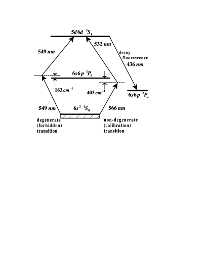
FIG. 1.: Excitation and detection schemes and relevant levels in atomic barium.

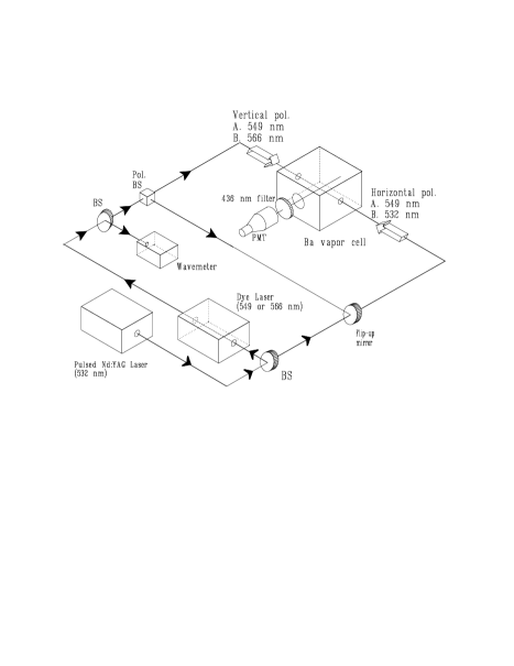
FIG. 2.: Schematic of the apparatus. BS=beamsplitter. For the forbidden transition, the dye laser is tuned around $549~{}nm$, and the flip-up mirror is in place as shown, so each of the counterpropagating beams in the vapor cell originates from the dye laser. For the calibration transition, the dye laser is tuned to $566~{}nm$ and the flip-up mirror is removed. The beam entering the vapor cell from the left then originates from the dye laser ($566~{}nm$), while the beam entering from the right originates from the Nd:YAG laser ($532~{}nm$).

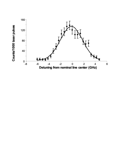
FIG. 3.: Typical scan through the nondegenerate calibration transition (points) and fit to determine peak height and linewidth (solid line). Taken with $230~{}\mu{}J/pulse$ at $566~{}nm$ and $0.4~{}\mu{}J/pulse$ at $532~{}nm$.

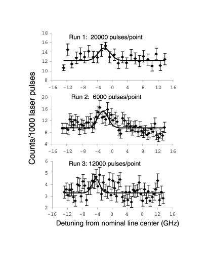
FIG. 4.: Scans through the degenerate transition and best fits to peak plus background.

REFERENCES

- [1] Present Address: MIT, Lincoln Laboratory, 244 Wood St, Lexington, MA, 02420.
- [2] Present Address: Physics Department, Bridgewater State College, Bridgewater, MA 02325
- [3] E. Ramberg and G. Snow, Phys. Lett. B 238, 438 (1990).
- [4] K. Deilamian, J.D. Gillaspy, and D.E. Kelleher, Phys. Rev. Lett. 74, 4787 (1995).
- [5] M. de Angelis, G. Gagliardi, L. Gianfrani, and G.M. Tino, Phys. Rev. Lett. 76, 2840 (1996).
- [6] R.C. Hilborn and C. Yuca, Phys. Rev. Lett. 76, 2844 (1996).
- [7] G. Modugno, M. Ignuscio, and G.M. Tino, Phys. Rev. Lett. 81, 4790 (1998).
- [8] See e.g. R.F. Streater and A.S. Wightman, PCT, Spin and Statistics, and All That (W.A. Benjamin, New York, 1964).
- [9] O.W. Greenberg and R.N. Mohapatra, Phys. Rev. D 39, 2032 (1989).
- [10] K.D. Bonin and T.J. McIlrath, J. Opt. Soc. Am. B 1, 52 (1984).
- [11] C.J. Bowers, D. Budker, E.D. Commins, D. DeMille, S.J. Freedman, A.-T. Nguyen, S.-Q. Shang, and M. Zolotorev, Phys. Rev. A 53, 3103 (1996).
- [12] J.J. Sakurai. Invariance Principles and Elementary Particles. (Princeton University Press, Princeton, 1964), pp. 15-16.
- [13] L.D. Landau, Dokl. Akad. Nauk. USSR 60, 207 (1948); C.N. Yang, Phys. Rev. 77, 242 (1950).
- [14] R. D. Amado and H. Primakoff, Phys. Rev. C 22, 1338 (1980).
- [15] O.W. Greenberg, Phys. Rev. Lett. 64, 709 (1990).
- [16] R. Hilborn and O.W. Greenberg, to be submitted.
- [17] O.W. Greenberg, Phys. Rev. D 43, 4111 (1991).
- [18] R. Hilborn, private communication.
- [19] D. Fivel, Phys. Rev. A 43, 4913 (1991).
- [20] O. W. Greenberg, in Workshop on Harmonic Oscillators, ed. D. Han, Y.S. Kim, and W.W. Zachary (NASA Conf. Pub. 3197, NASA, Greenbelt, MD, 1993).
- [21] O.W. Greenberg and R.C. Hilborn, Los Alamos e-print hep-th/9808106; submitted to Found. Phys.
- [22] A. Yu. Ignatiev, G.C. Joshi, and M. Matsuda, Mod. Phys. Lett. A 11, 871 (1996).
- [23] The correction factor takes into account the ratio of cross-sections for depletion of fluorescence at and ; this quantity was measured in a separate apparatus (D.E. Brown, D. Budker, D. DeMille, E. Deveney, and S. M. Rochester, to be published).
- [24] C.E. Moore, Atomic Energy Levels, Vol. III (NBS Circular No. 467: Washington, U.S. G.P.O., 1958).
- [25] B.M. Miles and W.L. Weise, Atom. Data 1, 1 (1969).
- [26] P. Hafner and W. Schwarz, J. Phys. B11, 2975 (1978).