Artificial Neural Network Modeling of Forest Tree Growth
by

Christopher Gordon
Research Report

Presented to the Faculty of Science of

The University of the Witwatersrand

in Partial Fulfillment

of the Requirements

for the Degree of

Master of Science

The University of the Witwatersrand

June 1998

Declaration

I declare that this research report is my own, unaided work. It is being submitted for the Degree of Master of Science in the University of the Witwatersrand, Johannesburg, South Africa. It has not been submitted before for any degree or examination in any other University.

Christopher Gordon
The University of the Witwatersrand June 1998

Abstract

The problem of modeling forest tree growth curves with an artificial neural network (NN) is examined. The NN parametric form is shown to be a suitable model if each forest tree plot is assumed to consist of several differently growing sub-plots. The predictive Bayesian approach is used in estimating the NN output.

Data from the correlated curve trend (CCT) experiments are used. The NN predictions are compared with those of one of the best parametric solutions, the Schnute model. Analysis of variance (ANOVA) methods are used to evaluate whether any observed differences are statistically significant. From a Frequentist perspective the differences between the Schnute and NN approach are found not to be significant. However, a Bayesian ANOVA indicates that there is a 93% probability of the NN approach producing better predictions on average.

Contents

toc

List of Tables

lot

List of Figures

lof

Chapter 1 Introduction

Growth curves are found in many different areas of study, e.g. in animals, plants, bacteria, fishes and populations. Their study is important in understanding what they are affected by and in predicting future values.

In the field of forestry much effort has been expended in finding mathematical models to describe the growth of trees Bredenkamp and Gregoire (1988), Seber and Wild (1989), Falkenhagen (1997). Models such as the logistic function have been proposed for predicting the average tree diameter at breast height (DBH) for a plot of forest trees:

$$y(t) = \frac{v}{1-\exp(-ut+a)}$$

$$= \operatorname{logistic}(t;u,v,a)$$

where $y(t)$ is the average DBH at age $t$ and $u$, $v$ and $a$ are the model parameters. For the model to be physically realistic:

(1.1) $$v,\,t\geq 0.$$

An advantage of such parametric models is that their parameters are easy to interpret, e.g. $v$ will be the maximum average DBH attainable. The disadvantage of such models is that they are only appropriate for modeling a very limited family of input/output mappings.

Multilayer perceptron artificial neural networks (NNs) Haykin (1994) provide a more flexible method of nonlinear regression. A general functional form of a NN for a one dimensional input to output mapping is given by:

(1.2) $$y(t)=\sum_{i=1}^{N_{h}}\operatorname{logistic}(t;u_{i},v_{i},a_{i})+b.$$

The larger $N_{h}$ is chosen to be, the more flexible the model. Hornik et al. (1990) have shown that equation (1.2) has fairly general function approximation qualities. In the case of modeling average forest tree growth, the NN model has a particularly suitable form. If the forest tree plot can be assumed to consist of $N_{h}$ groups of differently growing trees and each group’s average is modeled using the logistic function, then the NN functional form follows. However, the NN model does not usually contain the physical constraints mentioned in equation (1.1).

Thus, the NN model provides for heterogeneity in the growth of a forest tree plot. Unlike most NN applications, in mean forest tree growth modeling the NN functional form has some justification.

1.1 Artificial Neural Network Parameter Estimation

In order for the NN to have enough flexibility to fit a wide range of growth curves, $N_{h}$ has to be made fairly large. But a large $N_{h}$ implies many model parameters. The more model parameters, the more sensitive the solution is to any statistical variability in the data. This is known as the bias/variance dilemma.

Bayesian estimation provides a way of achieving a low bias without paying the price of a high variance. Predictions of unmeasured growth values are made by taking a weighted ‘sum’ of the predictions provided by all possible values of the parameters. Given $N$ input/output pairs, $\mbox{$\mathcal{D}$}=\{t_{1},y_{1};\ldots;t_{N},y_{N}\}$, a new measurement, $y_{N+1}$, is estimated by:

$$y_{N+1}=\int_{\mbox{$\mathcal{D}$}_{\theta}}y(t_{N+1};\theta)p(\theta|\mbox{$\mathcal{D}$})\,d\theta$$

where $\theta$ is the set of NN parameters and $\mbox{$\mathcal{D}$}_{\theta}$ is their domain. The weight of each prediction is given by the probability density function (pdf) of the network parameters given the data, $p(\theta|\mbox{$\mathcal{D}$})$. This pdf can factorized as follows:

$$p(\theta|\mbox{$\mathcal{D}$})\propto p(\mbox{$\mathcal{D}$}|\theta)p(\theta)$$

where $p(\theta|\mbox{$\mathcal{D}$})$ is known as the likelihood and expresses how the pdf is affected by the available data. The $p(\theta)$ component is known as the prior and expresses data ($\mathcal{D}$) independent knowledge about the model parameters. The prior can be used to include appropriate smoothness constraints which reduce the variance of the estimate.

1.2 Model Evaluation

When deciding which model is better at describing the process that generated a particular set of data, it is preferable to test the model on different data than it was trained on. Otherwise, the performance of each model is likely to be optimistically biased.

Using only one training set and test set to compare regression methods can be misleading. How well each method does will depend on the particular training and test cases used. The methods should be compared using many different training sets and test cases. Statistical hypothesis testing can then be used to determine which method is on average the best.

1.2.1 Correlated Curve Trend Experiments

A set of forest tree growth data suitable for the comparison of regression methods can be obtained from the results of what are known as the “correlated curve trend” (CCT) experiments O’Connor (1935). The growth of several different plots of trees with different initial and growing conditions was monitored. The growth measurements for the different plots can be used to provide an estimate of how well the NN approach performs on average in comparison with a parametric regression approach.

1.3 Objectives

In this report a survey of the available methods of forest tree growth curve modeling and Bayesian artificial neural networks (BNN) will be given. Statistical hypothesis testing will be used to compare the BNN approach with standard parametric models on the forest tree growth modeling problem.

Another of the aims of this research report is to evaluate the BNN approach on a practical, real world problem where a relatively small amount of data is available.

1.4 Outline

In Chapter 2 the previous literature on forest tree growth curve modeling is reviewed. The CCT experimental data are examined and the objectives of the curve fitting procedure are defined. The Schnute solution proposed by Falkenhagen (1997) is also discussed.

In Chapter 3 the Bayesian methodology used in the rest of the report is reviewed. Many of the relevant results are derived from first principles. The problems of defining prior distributions and the derivation of predictive distributions are discussed.

Chapter 4 surveys the relevant NN literature. The bias/variance dilemma is explained. The Bayesian treatment of Neal (1996) is summarized. A new justification for the prior distribution assigned to the network weights is given.

Chapter 5 reviews an analysis of variance (ANOVA) scheme, introduced by Rasmussen (1996), for comparing regression methods. A Bayesian hierarchical solution is also discussed.

In Chapter 6 the Bayesian neural network (BNN) scheme is applied to extrapolating the CCT data. The Frequentist ANOVA approach of Rasmussen (1996) and a hierarchical Bayesian ANOVA are used to compare the statistical significance of the Schnute and BNN results.

An overview of the results obtained in this research report is presented in Chapter 7. The scope and limitations of the results are discussed.

Chapter 2 Forest Tree Growth Modeling

If physics has its laws, biology has its variety. – G. A. Dover.

2.1 Background

There is a long history of forest tree growth modeling, from the first yield tables published over 200 years ago, to the recent Bayesian treatments of growth and yield models Vanclay (1995), Green and Strawderman (1996). Models help in forecasting timber yields, identifying appropriate treatments, planning how densely to plant trees together, deciding when to harvest and in monitoring the current state of a forest. They also help in determining the sustainability of various silviculture practices.

Vanclay (1995) has given a synthesis of the models and methods for tropical forests. An important aspect of tropical forest modeling is whether the timber harvesting is sustainable Vanclay (1994). Oshu (1991) uses a matrix model to predict long term tropical rain forest growth, in which matrix eigenvalues are used to estimate the intrinsic rate of natural increase. Methods of assessing the usefulness of permanent sample site databases are given in Vanclay et al. (1995).

Bayesian techniques have been used to estimate the parameters of a growth and yield model for slash pine plantations Green and Strawderman (1996). Posterior probability distributions were found for parameters such as number, volume and diameter of plantation trees. Zellner’s (1996) Bayesian method of moments was used to avoid having to make any assumptions about the form of the likelihood function. Another Bayesian paper is Green et al. (1994) where Bayesian estimation is used to fit the three parameter Weibull distribution to some tree diameter data. It is shown that the Bayesian solution avoids the negative location parameter estimates which plague the maximum likelihood solutions.

In a series of articles, Guan and Gertner (1991a; b; c; 1995) used an artificial neural network (see Chapter 4) to model forest tree mortality in terms of diameter at breast height (DBH) and the annual increment in DBH.

2.2 Correlated Curve Trend Experiments

The growth of a tree can be affected by competition from neighbouring trees for the available resources of sunlight, moisture, root space and soil nutrients Vanclay (1995). The degree of crowding has a considerable effect on the mean tree size.

O’Connor (1935) has examined the question of how the crowding of trees effects their growth. There are two components to this problem:

1. How closely the trees are planted together, known as the espacement.

2. What thinning strategies are employed.

There are a number of different qualities that a forester might consider when determining the optimum strategy:

1. The total volume of production, e.g. for pulp production.

2. How quickly the trees will grow.

3. The distribution of tree sizes.

The effects of different thinning regimes can be determined by keeping all other relevant factors constant and just varying the thinning regime. Generally the main factors in determining tree growth are the species of tree and the location or site where the trees are growing. Thus to compare different thinning regimes, the same forest tree species is planted on a site which is as uniform as possible.

The Correlated Curve Trend (CCT) experiments were based on the concepts of O’Connor (1935). A more modern view is given by Bredenkamp (1984). In the CCT experiments, the desired stand density is achieved by thinning in advance of competition. An analysis of one of these experiments, based on the growth of Eucalyptus grandis (Hill) Maiden, is given by Bredenkamp and Burkhart (1990). In their paper they evaluate the use of various ways of quantifying the degree of crowding within a plot.

Data from a CCT experiment established at the Border forest plantation in what is now known as Kwa-Zulu Natal, South Africa were used. In November 1936, test plots of Pinus roxburghii Sargent, a pine native to the Himalayas, were planted at an espacement of $1.80\times 1.80$ m Falkenhagen (1997). The area of each plot was 0.08 ha (800 $\mbox{m}^{2}$). A 29 m wide buffer zone of trees was planted around each plot. The geographical details of the plots are given in Table 2.1.

Latitude (S)	$30^{\circ}33^{\prime}$
Longitude (E)	$29^{\circ}45^{\prime}$
Altitude	1067 m
Average annual rainfall	945 mm
Length of dry season	3 months
Mean annual temperature	$16.1^{\circ}$C

Table 2.1: Geographical information of Border forest plantation in Kwa-Zulu Natal, South Africa (After Falkenhagen (1997).)

Twenty measurements of the diameter at breast height (DBH) of each tree were taken, see Appendix A. Measurements were usually taken during the summer months: October to March. At age 14, two measurements were taken, one in February and one in December. For this study these were averaged to give one measurement for that year. Height measurements were also made, but only diameter measurements will be examined in this report.

In Figure 2.1 all the tree measurements for plot 2 are displayed. The mean of the measurements is also plotted. Each mean point is joined to its neighbouring mean points by piece-wise straight line segments.

Figure 2.1: Individual growth curves for trees in plot 2.

The average DBH vs. time curves will be modeled for each plot. Figures 2.2 and 2.3 show the mean of the measured DBHs plotted against age for each plot used in this study. The number of trees in a plot at each measurement is also displayed as a vertical line at the age of each measurement.

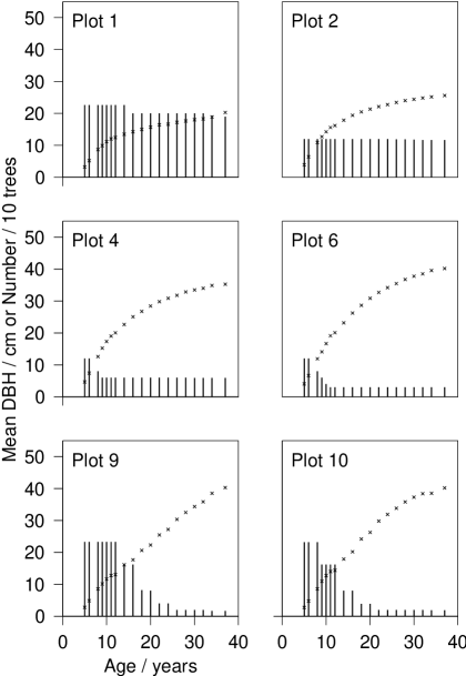
Figure 2.2: Forest tree mean density at breast height growth samples for plots 1 to 10. The $\times$’s represent the mean DBH measurements and the vertical lines, the number of trees.

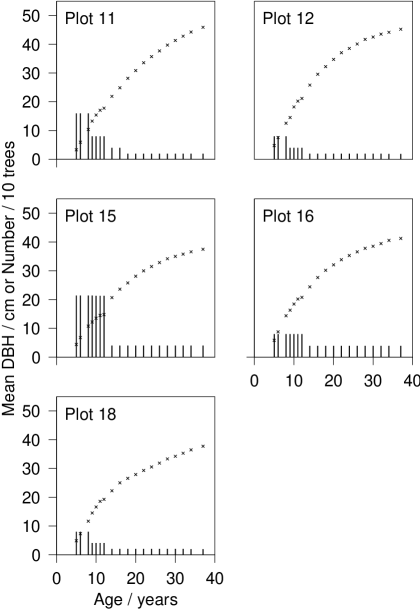
Figure 2.3: Forest tree mean density at breast height growth samples for plots 11 to 18. The $\times$’s represent the mean DBH measurements and the vertical lines, the number of trees.

As can be seen in some of the plots, a particularly drastic thinning can cause a discontinuity in the growth curve. This is particularly noticeable in plot 15.

In plot 1 the last few years of measurements actually show an increase in the rate of growth. This may be due to the natural decrease in trees within plot 1. Bredenkamp and Gregoire (1988) note a similar kind of behaviour in the Eucalyptus data which they studied.

2.3 Growth Curve Modeling

For modeling growth curve data, a large variety of models have been proposed. A review is given in Chapter 7 of Seber and Wild (1989). Approaches to growth curve modeling can be put into several different categories.

2.3.1 Linear Approach

This usually entails fitting polynomials to growth curves Kshirsagar (1976). Some of the polynomial coefficients can be assumed to be common for several different growth curves. Polynomial interpolation has been criticized as being biologically unreasonable Seber and Wild (1989). It is not commonly used in the forestry growth curve literature.

2.3.2 Autocorrelated Errors

Data which are collected from the same subjects at different times is known as longitudinal or time series data. Such data are often considered to have autocorrelated errors, Seber and Wild (1989). For example in modeling the growth in the weight of an animal, there might be a series of negative errors over a period of time that the animal was sick. For trees, correlated errors might be due to long periods of abnormal climatic conditions such as drought.

Presumably, the autocorrelation in errors is going to depend on the frequency of measurements. If the measurements are far enough apart there is unlikely to be any autocorrelation in errors. Also, stochastic analysis is easiest when there are equally spaced measurements, but there are ways of overcoming this restriction McDill and Amateis (1991).

In stochastic analysis, a difference function of the data is generally modeled by some differential form. In the next section, ways of modeling the data directly will be looked at. The basic differential forms the models are based on will also be discussed.

2.3.3 Nonlinear Models

Many nonlinear models have been proposed for growth curves. Some of them are based on biological principles. However, these biological motivations are not generally accepted as being compelling. Other models are purely empirical. The parameters of nonlinear growth curves can often be interpretable in terms of physical growth.

Exponential and Monomolecular Growth Curves

In the simplest of organisms, growth takes place by the binary splitting of cells. From which it follows that the rate of growth will be proportional to the current size of the organism, $f$:

$$\frac{df}{dt}=\kappa f,\text{ where }\kappa>0$$

which leads to the exponential growth curve:

$$f(t)=e^{\kappa(t-\gamma)}$$

where $\gamma$ is a constant. Many growth models are exponential for small time, $t$. However an exponential growth curve model leads to unlimited growth, whereas growth is known to stabilize:

$$\alpha=\lim_{t\rightarrow\infty}f(t),$$

which implies

$$\frac{df}{dt}\rightarrow 0\text{ as }t\rightarrow\infty.$$

A simple way of achieving this is by assuming that the growth rate is proportional to the remaining size:

$$\frac{df}{dt}=\kappa(\alpha-f)\text{ with }\kappa>0,$$

which has the general solution:

(2.1) $$f(t)=\alpha-(\alpha-\beta)e^{-\kappa t}.$$

If the function is used to describe monotonically increasing growth then

$$\alpha>\beta>0.$$

In this parameterization, $\alpha$ will be the final size, $\beta=f(0)$ is the initial size and $\kappa$ governs the rate of growth. Equation 2.1 is generally known as the monomolecular growth model.

Often in growth data, the growth first accelerates and then decelerates to a plateau. This gives rise to the “sigmoid” shaped growth curves. The point of inflection is the time when the growth rate is greatest.

The logistic model has the following differential equation:

$$\frac{df}{dt}=\frac{\kappa}{\alpha}f(\alpha-f),\text{ where $\kappa>0$ and $0<f<\alpha$}.$$

Here the $f$ in the numerator represents the tendency for the tree to grow indefinitely and the $\alpha-f$ represents the limiting component of the growth. Zeide (1993) shows how most growth equations can be broken up into an expansion and decline component. The general solution of the logistic model is

(2.2) $$f(t)=\frac{\alpha}{1+e^{-\kappa(t-\gamma)}},\quad-\infty<t<\infty.$$

The point of inflection occurs at $t=\gamma$ and the growth curve is symmetrical about this point.

The Richards Model

This restriction of the growth curve being symmetric about the point of inflection is not present in the Richards model Richards (1959). The differential equation for this model is given by:

$$\frac{df}{dt}=\frac{\kappa}{1-\delta}f\left[\left(\frac{f}{\alpha}\right)^{\delta-1}-1\right],\quad\delta\not=1,$$

which leads to the model given by:

$$f(t)=\alpha[1+(\delta-1)e^{-\kappa(t-\gamma)}]^{1/(1-\delta)},\quad\delta\not=1.$$

This equation has enjoyed extensive use in forest tree growth modeling. However, it has also been subject to much criticism. Ratowsky (1983) shows that its parameter estimates are unstable.

The Richards equation has an upper asymptote. Bredenkamp and Gregoire (1988) note that tree diameter growth can start to increase again after reaching what appears to be an upper asymptote, due to tree mortality.

The Schnute Model

An equation which is more stable than the Richards model and also allows the possibility of non-asymptotic growth was introduced by Schnute (1981). Unlike most other growth models, the Schnute model is based on the acceleration of growth:

(2.3) $$\frac{d^{2}f}{dt^{2}}=\left(k_{1}+\frac{k_{2}}{f}\right)\frac{df}{dt}.$$

The integrated version of the Schnute model is given by:

(2.4) $$f(t)=\left[f_{1}^{b}+(f_{2}^{b}-f_{1}^{b})\frac{1-e^{-a(t-\tau_{1})}}{1-e^{-a(\tau_{2}-\tau_{1})}}\right]^{1/b}$$

where

$$t =\text{age of interest}$$

$$\tau_{1} =\text{youngest measured age}$$

$$\tau_{2} =\text{oldest measured age}$$

$$f_{1} =f(\tau_{1})$$

$$f_{2} =f(\tau_{2})$$

$$a =\text{constant acceleration in growth rate}$$

$$b =\text{incremental acceleration in growth rate.}$$

In fitting the Schnute model the initial guesses for $f_{1}$ and $f_{2}$ are the initial and final measured size values.

2.3.4 Estimation Methods

Usually each growth measurement is assumed to have been drawn from a Normal distribution:

(2.5) $$y_{i}|t_{i},\theta\sim\operatorname{Normal}(f(t_{i},\theta),\sigma^{2}).$$

If data, $\{y_{i},t_{i}\}\equiv\{(y_{1},t_{1});(y_{2},t_{2});\dots;(y_{N},t_{N})\}$, are available then the maximum likelihood estimate (mle) of the parameters $\theta$ is given by:

$$\theta_{\operatorname{mle}} =\max_{\theta}p(\{y_{i}\}|\{t_{i}\},\theta)$$

$$=\max_{\theta}\exp-\sum_{i=1}^{N}(y_{i}-f(t_{i},\theta))^{2}$$

(2.6) $$=\min_{\theta}\sum_{i=1}^{N}(y_{i}-f(t_{i},\theta))^{2}$$

i.e. in this case the maximum likelihood parameter estimates are found by minimizing the mean square error (MSE) of the predicted diameters by iterative numerical methods.

Given $\theta$, the errors, $e_{i}=y_{i}-f(t_{i},\theta)$, are assumed to be independent. Thus, one diagnostic of the model fit is given by plotting the residuals and seeing if there is any unusual pattern of runs of positive and negative residuals, Draper and Smith (1981).

2.4 Modeling of Pinus Roxburghii Data

Falkenhagen (1997) has studied nine different growth models for the diameter growth of the Pinus Roxburghii data discussed in Section 2.2. He found that the Schnute model, equation (2.4) had the least problems with convergence and gave the overall minimum mean square error.

Zeide (1993) noted that the differential form of Schnute’s model (equation (2.3)) does not provide a good fit for a Norway spruce tree data set. However, as the objective is to fit the integrated form of Schnute’s model (2.4), this is not strictly relevant.

A good fit is obtained when all the data in each plot’s data set is used Falkenhagen (1997). Thus the Schnute model adequately interpolates the data. Falkenhagen (1997) also found the errors in the interpolation showed little autocorrelation (i.e. there were no unusually long runs of positive and negative residuals), thus indicating that stochastic analysis (Section 2.3.2) may be unnecessary. A more difficult problem would be to see how well the model extrapolates the data. Thinning continued in some cases until the age of 24. It is pointless trying to extrapolate the tree growth while thinning is still taking place as then the model would have to predict the occurrence of any future thinning. As only age will be used as an explanatory variable, this would not be possible. Thus it will be required that the model extrapolate from age 30 years onwards. By which time the tree has resumed normal growth.

As will be seen in Chapter 6, the Schnute model provides poor extrapolations for some plots and thus other modeling techniques need to be investigated.

Chapter 3 Bayesian Statistics

Probability, then, can be thought of as the mathematical language of uncertainty. R. L. Winkler

In this report Bayesian Statistics will be used in Neural Network Modeling, see Chapter 4, and in comparing the performance of different regression techniques, see Chapter 5. In this chapter all the Bayesian theory which is relevant to later work will be reviewed. Many aspects of Bayesian Statistics which will not be relevant to the rest of this report will not be discussed. Some of the results of examples in this chapter will be relevant to later developments.

There are many text books on Bayesian Statistics, for example those written by Berger (1985), Press (1989), Box and Tiao (1992), Bernardo and Smith (1994), Gelman et al. (1995) and Jaynes (1996). Several, such as the book written by Jaynes (1996), assume very little statistical training. The books by Box and Tiao (1992) and Jaynes (1996) are more oriented towards the natural sciences.

3.1 Foundations

Broadly speaking there are two schools of Statistics, Bayesian and Frequentist (also known as Classical or Orthodox). The Bayesian school is a minority, but has seen rapid growth in the last few decades.

Frequentists generally only use probabilities to describe the proportion of times an event will occur in a given population. For example, if a rod is measured, a Frequentist will not consider its true length as a random variable. However, if there is a whole assembly line of rods then the length of the different rods within the assembly line can be assigned a random variable. A Classical view of the Bayesian / Frequentist debate is given by Papoulis (1990).

Bayesians on the other hand use probability to express all types of uncertainty. A probability of zero corresponds to an impossible event and a probability of one to a certain event. Probabilities between zero and one express the degree of uncertainty. So in the Bayesian framework it is possible to pose questions such as “What is the probability of a theory being true?”

In a Bayesian sense, random variables are used to express uncertainty. Probabilities can be given for different proposed values of the variable. In Bayesian Statistics, model parameters are treated as random variables.

3.2 The Rules of Probability

A system for dealing with uncertainty that satisfies a certain number of reasonable desired properties, must be consistent with the following two rules Jaynes (1996):

Product Rule :

(3.1) $$P(AB|C)=P(A|BC)P(B|C)=P(B|AC)P(A|C).$$

Sum Rule :

(3.2) $$P(A|B)+P(\bar{A}|B)=1$$

where $A$, $B$ and $C$ are propositions, e.g.

$$A = X x_{l} x_{u}$$ A measurement of a quantity will lie somewhere between and .

$$B = \{x_{1},x_{2},\ldots,x_{n}\} X$$ The samples are measurements of .

$$C = X$$ A Gaussian probability distribution function should be used for .

The notation $P(AB|C\bar{D})$ reads the probability of $A$ and $B$ being true given that $C$ is true and $D$ is false. A proposition is a statement that can be either true or false. Prior information will generally be denoted by an $I$.

Since a continuous variable can take on an infinite number of values, its probability of being any particular number is infinitely small. Thus when dealing with random variables it is useful to work with a probability density function (pdf). The pdf for a variable $X$ is defined as:

(3.3) $$p(x|I)\equiv\frac{d}{dx}P(X\leq x|I).$$

Multivariate pdfs are defined in a similar way:

$$p(x,y|I)\equiv\frac{\mbox{$\partial$}}{\mbox{$\partial$}y}\frac{\mbox{$\partial$}}{\mbox{$\partial$}x}P(X\leq x,Y\leq y|I).$$

The pdf, $p(x|I)$, is just a function of $x$. Note that it could well have a different functional form to $p(y|I)$. To distinguish the functional form, a subscript will be used. E.g. $p_{X}(x^{2}|I)$, which is just the same function as $p(x|I)$ except with all the $x$’s replaced by $x^{2}$’s. A random variable $X$ has been distinguished from an instance of that variable, $x$. However, the same symbol will usually be used for the random variable and for an instance of that variable, but the meaning should be clear from the context.

It follows from the definition of pdfs, equation (3.3), that they must always be positive. The probability of a variable taking on a value contained in $\mbox{$\mathcal{D}$}^{\prime}$, which is a subset of the whole domain of the variable, $\mathcal{D}$, is given by

$$P(X\in\mbox{$\mathcal{D}$}^{\prime})=\int_{x\in\mbox{$\mathcal{D}$}^{\prime}}p(x)\,dx.$$

From the sum rule, equation (3.2), it follows that

$$P(X\in\mbox{$\mathcal{D}$}^{\prime})+P(X\not\in\mbox{$\mathcal{D}$}^{\prime})=1.$$

From which it follows that

(3.4) $$\int_{x\in\mbox{$\mathcal{D}$}}p(x)\,dx=1.$$

In the above, the probabilities have not been conditioned on any prior information, however all probabilities are based on some prior information and when it is not explicitly stated, it is assumed. Jaynes (1996) discussed the importance of bearing in mind the prior information a probability is based on.

3.3 Bayes’ Rule

Using the product rule, equation (3.1), Bayes’ rule can easily be deduced:

(3.5) $$P(A|B)=\frac{P(B|A)P(A)}{P(B)}.$$

Many problems solved by Bayesian analysis take on the following form:

1. Some data $x=\{x_{1},\ldots,x_{n}\}$ are available.

2. A pdf, $p(x|\theta)$ is proposed, where $\theta=\{\theta_{1},\theta_{2}\}$, are a number of unknown model parameters. This pdf is known as the likelihood. It contains all the information about how the parameters are related to the data.

3. A prior pdf, $p(\theta)$, which reflects the available prior information, is chosen.

Writing Bayes rule in terms of the above pdfs, gives:

(3.6) $$p(\theta|x)=\frac{p(x|\theta)p(\theta)}{p(x)}.$$

The pdf, $p(\theta|x)$ is known as the posterior distribution of $\theta$.

3.4 The Predictive Distribution

The posterior pdf $p(\theta|x)$ must be normalized, i.e.

$$\int_{\theta\in\mbox{$\mathcal{D}$}_{\theta}}p(\theta|x)\,d\theta=1.$$

Using Bayes rule, equation (3.6), in the above equation, it follows that

$$\int_{\theta\in\mbox{$\mathcal{D}$}_{\theta}}\frac{p(x|\theta)p(\theta)}{p(x)}\,d\theta=1.$$

From which the marginal pdf, $p(x)$ can be evaluated:

(3.7) $$p(x)=\int_{\theta\in\mbox{$\mathcal{D}$}_{\theta}}p(x|\theta)p(\theta)\,d\theta.$$

Note that $p(x)$ depends on the form chosen for the likelihood and the prior. One should write $p(x|I)$, where the $I$ specifies the functional forms chosen for $p(\theta|x,I)$ and $p(\theta|I)$. So given different prior information (assumptions), $I_{1}$ and $I_{2}$, the functional forms of $p(x|I_{1})$ and $p(x|I_{2})$ can be very different.

The pdf, $p(x|I)$, is usually known as the predictive distribution, as it gives the probability density function of any new measurement of data. When conditioned only on the prior information, $p(x|I)$ is the prior pdf for the data. To get the pdf of some new data, $x_{n+1}$, given some old data $\{x_{1},\ldots,x_{n}\}$, the predictive distribution is as follows:

(3.8) $$p(x_{n+1}|\{x_{1},\ldots,x_{n}\},I)=\int_{\theta}p(x_{n+1}|\theta,I)p(\theta|\{x_{1},\ldots,x_{n}\},I)\,d\theta.$$

The pdf, $p(x|I)$ is also referred to as the evidence, (see MacKay 1992a; b). The reason for this is that it can be used to compare hypotheses. Say you have two hypotheses (theories) $H_{1}$ and $H_{2}$, and some data $x$. In order to compare the two hypotheses, in light of the data $x=\{x_{1},\ldots,x_{n}\}$, the posterior odds ratio can be evaluated:

$$\frac{P(H_{1}|x,I)}{P(H_{2}|x,I)}=\frac{p(x|H_{1},I)P(H_{1}|I)}{p(x|H_{2},I)P(H_{2}|I)}.$$

So $p(x|H,I)$ indicates how much the data contribute to the probability of $H$ being true, i.e. what evidence it provides for $H$. An interesting example is given in Jefferys and Berger (1992), where a fudged Newtonian theory and Einstein’s Theory of General Relativity are compared in this manner.

3.5 Eliminating Nuisance Parameters

If one is interested in all the parameters, $\theta$, then the posterior pdf of equation (3.6) gives all the available information about $\theta$ given the prior information and the data. For instance, the probability of the parameters being in a particular region $\mbox{$\mathcal{D}$}^{\prime}$ is given by

$$P(\theta\in\mbox{$\mathcal{D}$}^{\prime}|x,I)=\int_{\theta\in\mbox{$\mathcal{D}$}^{\prime}}p(\theta|x,I)\,d\theta.$$

This will not usually coincide with Frequentist confidence intervals. However, if only a portion of the parameters, $\theta_{1}$, are of interest and the rest of the parameters, $\theta_{2}$, are nuisance parameters, then the pdf for the parameters of interest can be obtained by

$$p(\theta_{1}|x,I) =\int_{\theta_{2}\in\mbox{$\mathcal{D}$}_{\theta_{2}}}p(\theta_{1},\theta_{2}|x,I)\,d\theta_{2}$$

(3.9) $$=\int_{\theta_{2}\in\mbox{$\mathcal{D}$}_{\theta_{2}}}p(\theta_{1}|\theta_{2},x,I)p(\theta_{2}|x,I)\,d\theta_{2}.$$

This relationship follows from the general form of equation (3.7).

3.6 Prior Probability Density Functions

In this section, methods of choosing the prior $p(\theta)$ are discussed. There are many ways of choosing the prior, and Berger (1985) has given a comprehensive review. Only those that will be relevant to the problems that will be solved in this research report will be looked at.

3.6.1 Non-Informative Priors

Often in scientific work, it is considered desirable not to include any information in the prior pdf, $p(\theta)$. The interest is in what the data imply about $p(\theta|x)$. Also there may simply be no useful prior information about the values of the parameters.

From Bayes’ rule,

$$p(\theta|x)\propto p(\theta)p(x|\theta).$$

The posterior is only effected by the data via the likelihood function, $p(x|\theta)$. So if one does not in any way want to distort the effect of the likelihood, the prior should be as flat as possible in the areas where the likelihood has an appreciable value and not have any relatively large fluctuations outside that area. For instance, if the prior had a peak in the tails of the likelihood, that could lead to an appreciable peak in the posterior. Also, if the prior was varying rapidly across the area where the likelihood had most of its mass, this would distort the shape of the likelihood. So, qualitatively speaking, non-informative priors should be as broad and featureless as possible. For a more detailed discussion on the qualities a prior should have see Berger (1985).

In cases where little or no prior information will be used, many Orthodox Statisticians argue that Bayesian methods are not appropriate. In the Maximum Likelihood method, parameters are chosen which maximize the probability of the data, e.g.

(3.10) $$\theta_{\mbox{mle}}=\max_{\theta}p(x|\theta).$$

However, this is the same as making a maximum a posterior (MAP) estimate and choosing a uniform prior for the parameters. The uniform prior is given by

(3.11) $$p(\theta)=a$$

where $a$ is some constant. This prior cannot be normalized as in equation (3.4), it is therefore said to be improper. A uniform prior can be thought of as the limit of a Gaussian prior as the variance goes to infinity. Improper priors can still lead to proper posteriors:

(3.12) $$p(\theta|x)=\frac{p(x|\theta)}{\int p(x|\theta)\,d\theta}$$

where the constant, $a$, cancels out in the denominator and numerator.

In the Bayesian approach, equation (3.12), the whole pdf of $\theta$ is obtained. To obtain a point estimate, as in the Maximum Likelihood case, equation (3.10), a loss function is needed, see Section 3.7.

The Problem with Uniform Priors.

One difficulty in assuming that $p(\theta)$ is uniform, is that if some one to one function of $\theta$ is of interest, $\phi=f(\theta)$, then $p(\phi)$ will not in general be uniform. In order to determine the pdf of a function of a parameter, the following formula can be used Papoulis (1990):

(3.13) $$p_{\phi}(\phi)=p_{\theta}(\phi)\mbox{ $\displaystyle\left|\frac{df^{-1}(\phi)}{d\phi}\right|$ },$$

where $f^{-1}(\phi)$ denotes the inverse function of $f(\phi)$. For clarity, subscripts are being used to distinguish the different functional forms of $p(\cdot)$. For example, if $\phi=\theta^{-1}$ then

$$p_{\phi}(\phi)=\phi^{-2}p_{\theta}(\phi).$$

So, if $p_{\theta}(\theta)=1$, then $p_{\phi}(\phi)=\phi^{-2}$. Thus, by assuming complete uncertainty about where $\theta$ is, it is assumed that $\theta^{-1}$ is more likely to be closer to zero than further away. If, instead, $\theta^{-1}$ was initially the parameter of interest, then the reverse would hold. Thus, the priors assigned to all the different functions of $\theta$ are completely determined by which function of $\theta$ the uniform prior is assigned to. This is undesirable, since the choice of which function of $\theta$ to assign the uniform prior to is fairly arbitrary.

Jeffreys’ Priors

As soon as a prior is assigned to some function of $\theta$, this automatically implies what priors are assigned to all other one to one functions of $\theta$, via equation (3.13). To make this whole family of priors invariant to which function of $\theta$ was initially selected, the Jeffreys’ prior can be used:

(3.14) $$p(\theta)\propto[\mbox{$\mathcal{J}$}(\theta)]^{1/2},$$

where $\mbox{$\mathcal{J}$}(\theta)$ is the Fisher Information for $\theta$ Bernardo and Smith (1994):

$$\mbox{$\mathcal{J}$}(\theta) =-\int_{x}\frac{d^{2}\log(p(x|\theta))}{d\theta^{2}}p(x|\theta)\,dx$$

(3.15) $$=-E\left[\left.\frac{d^{2}\log(p(x|\theta))}{d\theta^{2}}\right|\theta\right],$$

where $E[\cdot|\cdot]$ is the conditional expectation. Once the Jeffreys’ prior has been assigned to $\theta$, then any one to one function of $\theta$, such as $\phi=f(\theta)$ is also assigned a Jeffreys’ prior:

$$[p_{\mbox{$\mathcal{J}$}}(\phi)]^{2} \propto\mbox{$\mathcal{J}$}(\phi)$$ by defn. equation (3.14)

$$=-E\left[\left.\frac{d^{2}\log p(x|\phi)}{d\phi^{2}}\right|\phi\right]$$ by equation (3.15)

$$=-E\left[\left.\frac{d^{2}\log p(x|\theta=f^{-1}(\phi))}{d\theta^{2}}\mbox{ $\displaystyle\left|\frac{d\theta}{d\phi}\right|$ }^{2}\right|\phi\right]$$ by the chain rule

$$=\mbox{$\mathcal{J}$}(\theta)\mbox{ $\displaystyle\left|\frac{d\theta}{d\phi}\right|$ }^{2} \text{by equation \eqref{eq:Fisher} },$$

from which it follows that

$$p_{\mbox{$\mathcal{J}$}}(\phi)=p_{\mbox{$\mathcal{J}$}}(\theta)\mbox{ $\displaystyle\left|\frac{d\theta}{d\phi}\right|$ },$$

where the $\mathcal{J}$ subscript is used to indicate that the prior was formed by Jeffreys’ procedure, equation (3.14). As can be seen from equation (3.13), this is how pdfs should transform when a function of a parameter is taken. Thus, by choosing Jeffreys’ prior for one function of $\theta$, all other functions of $\theta$ are assigned their own Jeffreys’ priors.

Box and Tiao (1992) and Bernardo and Smith (1994) give further justifications for assigning Jeffreys’ priors.

As an example, if the likelihood is a Gaussian, $p(x|\theta)=\operatorname{Normal}(\mu,\sigma^{2})$, and $\sigma$ is assumed known, then using equation (3.14) it can be seen that the Jeffreys’ prior for $\mu$ is $p(\mu)=1$. If instead the mean, $\mu$, is assumed known then the Jeffreys’ prior for $\sigma$ is $p(\sigma)=\sigma^{-1}$.

Jeffreys’ prior can also be extended to multi-parameter problems:

(3.16) $$p(\theta)=\mbox{ $\displaystyle\left|J\right|$ }^{1/2}$$

where $\displaystyle\left|J\right|$ is the determinant of the Fisher information matrix defined by:

(3.17) $$J_{i,j}=\int_{x}\frac{\partial^{2}p(\theta|x)}{\partial\theta_{i}\partial\theta_{j}}\,dx,$$

where $\theta_{i}$ is the $i$th parameter of the vector of parameters $\theta$.

There are cases when Jeffreys’ priors do not give good results for multi-parameter models. For instance in the case of a Gaussian distribution, $p(x|\theta)=\operatorname{Normal}(\mu,\sigma^{2})$, where both $\mu$ and $\sigma$ are unknown, the Jeffreys’ prior is $p(\mu,\sigma)=1/\sigma^{2}$. This leads to a posterior with undesirable properties, as shown on pg. 361 of the book by Bernardo and Smith (1994).

One ad-hoc procedure that has been proposed for overcoming such problems, is to assume some of the parameters are a priori independent. So in the case of the prior for $p(\mu,\sigma)$, for a normal likelihood:

$$p(\mu,\sigma) =p(\mu|\sigma)p(\sigma)$$

$$=p(\mu)p(\sigma)$$

$$=1/\sigma$$

where the single parameter Jeffreys’ priors, equation (3.14), are used for $p(\mu)$ and $p(\sigma)$. This prior leads to a posterior with more acceptable properties.

Another approach called reference priors has been developed, Bernardo and Smith (1994), which reduces to a Jeffreys’ prior in the single continuous parameter case and does not have some of the problems associated with Jeffreys priors in the multi-parameter case. However, reference priors are beyond the scope of this report.

3.6.2 Conjugate Priors

In general, the posterior, $p(\theta|x)$, and the evidence, $p(x)$, are not easy to evaluate. Thus, it can be desirable to choose the prior, $p(\theta)$, such that the necessary calculations will be made easier. Usually any prior knowledge that is available is of a vague form and so the form of the prior pdf is fairly arbitrary, provided its properties are consistent with the available prior knowledge.

One suggestion is to find a prior pdf which when combined with the likelihood function leads to a posterior pdf with the same form as the prior pdf. These are called conjugate priors. They have the added advantage that they lead to a more interpretable posterior.

Example 3.1

Consider the case where $x$ is normally distributed with a known mean $\mu$ and a standard deviation of $\sigma$, i.e.  $x\sim\operatorname{Normal}(\mu,\sigma^{2})$. Instead of working with the standard deviation, the precision $\tau=1/\sigma^{2}$ will be used. It doesn’t matter what function of the parameter is used because one can always transform back to the function of interest using equation (3.13). If $x$ consists of $N$ measurements, then the likelihood is given by:

$$p(x|\mu,\sigma) =p(x_{1},x_{2},\ldots,x_{N}|\mu,\sigma)$$

(3.18) $$=\prod_{i=1}^{N}p(x_{i}|\mu,\sigma)$$

$$=\left(2\pi\sigma^{2}\right)^{-N/2}\exp\left(-\sum_{i}(x_{i}-\mu)^{2}/(2\sigma^{2})\right),$$

where in equation (3.18) it is assumed that each measurement is independent of every other measurement, given that $\mu$ and $\sigma$ are known. Expressing the likelihood in terms of the precision, $\tau$, gives:

$$p(x|\mu,\tau) \propto\tau^{N/2}\exp\left(-\tau\sum_{i}(x_{i}-\mu)^{2}/2\right)$$

(3.19) $$\propto\tau^{N/2}\exp\left(-\tau Ns^{2}/2\right),$$

where

(3.20) $$s^{2}=\frac{1}{N}\sum_{i}(x_{i}-\mu)^{2}$$

is the sample variance. Note that any constants of proportionality in the likelihood are not necessary because the posterior will be normalized at a later stage anyway. If the functional form of the pdf in equation (3.19) is looked at with $\tau$ as the variable and everything else as constants, then it is a Gamma distribution in $\tau$. Assume the prior for $\tau$ is a Gamma distribution:

(3.21) $$p(\tau|\alpha,\omega)=\frac{(\alpha/2\omega)^{\alpha/2}}{\Gamma(\alpha/2)}\tau^{\alpha/2-1}\exp(-\tau\alpha/(2\omega))I_{(0,\mbox{$\infty$})}(\tau),$$

where

(3.22) $$I_{(0,\mbox{$\infty$})}(\tau)=\left\{\begin{array}[]{ll}1,&\tau\in(0,\mbox{$\infty$})\\ 0,&\tau\not\in(0,\mbox{$\infty$})\end{array}\right.$$

ensures the probability is only non-zero for positive values of $\tau$. The parameters $\alpha$ and $\omega$ must satisfy $\alpha>0$ and $\omega>0$. The mean of the Gamma distribution is given by

(3.23) $$E(\tau|\alpha,\omega)=\omega$$

and the variance is given by

(3.24) $$\mbox{Var}(\tau|\alpha,\omega)=2\omega^{2}/\alpha.$$

The parameters $\alpha$ and $\omega$ can be chosen to correspond to the desired prior mean and variance. Using equation (3.21) for the prior, the posterior of $\tau$ is given by:

(3.25) $$p(\tau|x,\mu,\alpha,\omega)\propto\tau^{(N+\alpha-2)/2}\exp\left(-\frac{1}{2}\tau(\alpha/\omega+Ns^{2})\right).$$

The posterior is also a Gamma pdf. Thus equation (3.21) is a conjugate prior to the likelihood given in equation (3.19). One advantage of conjugate priors is that it is easy to interpret the role played by the prior in the posterior. As can be seen in equation (3.25), $\alpha$ plays the same role as $N$ and $1/\omega$ plays the same role as $s^{2}$. Thus one could interpret the prior, $p(\tau|\alpha,\omega)$, as being equivalent to $\alpha$ measurements which have a sample variance of $1/\omega$. From which it follows that a natural interpretation for $1/\omega$ is the prior variance of $x$.

In Section 4.7 of Chapter 4 a Gamma prior will be used for the precision of some model parameters and model noise.

3.6.3 Empirical Bayes

In empirical Bayes methods the data are used in estimating the prior. In Section 3.4 it was shown how the marginal distribution of the data, $p(x|H,I)$, contributes to the probability of the hypothesis being true:

$$p(H|x,I)\propto p(H|I)p(x|H,I).$$

The hypothesis, $H$, consists of two components: the likelihood, $\mathcal{L}$, and the prior, $\pi$. The type II maximum likelihood (ML-II) prior is obtained by maximizing the likelihood of the prior:

$$\pi=\max_{\pi}p(x|\pi,\mbox{$\mathcal{L}$},I).$$

Usually the maximization is done over some restricted family of priors. Using ML-II priors violates Bayes’ rule since the prior is no longer independent of the data. However they can be used as an approximation to a true Bayesian approach. Berger (1985) elaborates on this distinction.

Example 3.2

Given the prior, $p(\theta|\tau)=\operatorname{Normal}(0,1/\tau)$, then a suitable value of $\tau$ has to be chosen. Using the ML-II method,

$$\tau =\max_{\tau}p(x|\tau,I)$$

(3.26) $$=\max_{\tau}\int_{\theta}p(x|\theta,I)p(\theta|\tau,I)\,d\theta.$$

Parameters, like $\tau$, which determine the prior distribution are known as hyperparameters.

One of the problems with the ML-II method is that it does not acknowledge any uncertainty there may be in choosing the hyperparameters of a prior distribution. In the next section it will be shown how this additional uncertainty can be included.

3.6.4 Hierarchical Priors

Given the functional form for a prior distribution, $p(\theta|\tau,I)$ without known values for the hyperparameters, $\tau$, then a prior can be assigned to $\tau$ which reflects any uncertainty about its value.

Example 3.3

Using the same prior as in Example 3.2, but instead of assigning the ML-II value for $\tau$, a prior is assigned to $\tau$. Choosing a conjugate prior gives

$$p(\tau|I)=\mbox{Gamma}(\alpha,\omega).$$

Values now have to be assigned for $\alpha$ and $\omega$ which reflect the prior uncertainty in $\tau$.

The following derivation shows the relationship between the hierarchical and ML-II priors:

$$p(\theta|x) =\int_{\tau}p(\theta,\tau|x)\,d\tau$$

$$=\int_{\tau}p(\theta|\tau,x)p(\tau|x)\,d\tau$$

(3.27) $$=\int_{\tau}p(\theta|\tau,x)\frac{p(\tau)p(x|\tau)}{p(x)}\,d\tau.$$

From which can be seen that the ML-II method is equivalent to making the following approximation:

$$p(x|\tau)\approx c\delta(\tau-\tau_{\mbox{mle}}),$$

where $\tau_{\mbox{mle}}$ is the maximum likelihood estimate of $\tau$ and $c=p(\tau_{\mbox{mle}})/p(x)$ is a scaling factor. Thus the ML-II method only uses the maximum of the likelihood, $p(x|\tau)$, while hierarchical priors make use of the whole likelihood function.

It is always possible to integrate out the hierarchical prior to get a single level prior:

$$p(\theta)=\int_{\tau}p(\theta|\tau)p(\tau)\,d\tau.$$

One advantage of using hierarchical priors is that they generally are equivalent to single level priors which have very flat tails. This means they are robust, i.e. the final posterior does not depend strongly on the precise form, e.g. the mean and variance, of the hyperprior Berger (1985). So the final result should not be too sensitive to the values chosen for $\alpha$ and $\omega$ in Example 3.3.

3.6.5 Exchangeable Parameter Priors

Another use for hierarchical priors is when one has several parameters which are exchangeable. By exchangeable it is meant that one has no prior knowledge for distinguishing or grouping one or more of the parameters from the others. Probabilistically, this can be represented as the prior, $p(\theta_{1},\theta_{2},\ldots,\theta_{N})$, being invariant to permutations of the parameters Gelman et al. (1995). The simplest form of an exchangeable distribution is to have each parameter, $\theta_{i}$, independently and identically drawn from a distribution which has hyperparameters $\tau$:

(3.28) $$p(\theta|\tau)=\prod_{i=1}^{N}p(\theta_{i}|\tau).$$

In general the hyperparameter $\tau$ is not known and so it is necessary to integrate over the uncertainty in $\tau$:

$$p(\theta)=\int_{\tau}\prod_{i=1}^{N}p(\theta_{i}|\tau)p(\tau)\,d\tau,$$

where $p(\tau)$ is a hierarchical prior. After integrating out the hyperparameter $\tau$, the parameters in $p(\theta)$ will not in general be independent, i.e.

$$p(\theta_{i}|\theta_{1},\ldots,\theta_{i-1},\theta_{i+1},\ldots,\theta_{N})\not=p(\theta_{i}).$$

This provides a good remedy to the problem of overfitting, which will be discussed in Section 4.5 of Chapter 4.

Example 3.4

Consider the weighted sum,

$$y(t)=\sum_{i}u_{i}f_{i}(t)+\epsilon$$

where $\epsilon$ is the component of $y(t)$ which is not explained by $t$, otherwise known as the noise. If the prior values of $f_{i}(t)$ are independent of $i$ then the weights $u_{i}$ can be modeled as exchangeable. Therefore the posterior pdf is given by:

$$p(\theta|\{y,t\})=\int_{\tau}p(\theta|\{y,t\},\tau)p(\tau|\{y,t\})\,d\tau.$$

Since $\tau$ will determine the dependence between the weights, and $\tau$ will be determined by the data through $p(\tau|\{y,t\})$, it follows that the dependence between the weights is determined by the data.

3.7 Loss Functions

Generally a Bayesian analysis will result in a posterior pdf, either for a parameter of interest or for a future data value. It may be desirable to just report a single guess for the parameter rather than the whole posterior pdf. In which case it is necessary to decide which value to report. There is an extensive Bayesian theory on how to make these decisions Berger (1985).

In Bayesian decision theory a loss is associated with any decision. For instance, if one is trying to guess the value of some parameter $\theta$, then the loss associated with a guess, $\theta^{*}$, is a function, $l(\theta,\theta^{*})$. There are many possible choices for $l(\cdot,\cdot)$ depending on the application. A common choice is the square error loss function:

$$l(\theta,\theta^{*})=(\theta-\theta^{*})^{2}.$$

Another common choice is to use the absolute error. In Bayesian decision theory the optimum decision is given by choosing the value, $\theta^{*}$, which minimizes the expected loss:

$$\theta^{*}=\min_{\theta^{*}}E[l(\theta,\theta^{*})].$$

For the square error loss function:

$$\theta^{*} =\min_{\theta^{*}}E[(\theta-\theta^{*})^{2}]$$

$$=\min_{\theta^{*}}\int_{\theta}(\theta-\theta^{*})^{2}p(\theta)\,d\theta$$

from which it follows:

$$\frac{\partial}{\partial\theta^{*}}\int_{\theta}(\theta-\theta^{*})^{2}p(\theta)\,d\theta=0$$

$$\int_{\theta}(\theta-\theta^{*})p(\theta)\,d\theta=0$$

(3.29) $$\theta^{*}=\int_{\theta}\theta p(\theta)\,d\theta.$$

Thus when a square error loss function is used, the optimum value to choose is the posterior mean of the parameter.

The zero-one loss function, is zero if the guess is correct, $\theta^{*}=\theta$, and one otherwise. Its minimum expected loss is evaluated by setting $\theta^{*}=\max_{\theta}p(\theta|x)$, i.e. the maximum a posteriori value. It follows that the maximum likelihood method is a special case of Bayesian estimation, with uniform priors and a zero-one loss function. It seems advantageous that the Bayesian approach makes use of the whole likelihood function when making point estimates, while the Frequentist approach only uses the maximum of the likelihood function.

3.8 Bayesian Computation

As has been shown, many Bayesian calculations involve solving integrals, for example:

1. Obtaining posterior pdfs can involve integrating out nuisance parameters (see Section 3.5), e.g.

   (3.30) $$p(\tau|x)=\int_{\gamma}p(\tau,\gamma|x)\,d\gamma,$$

   where $\gamma$ could be one or more nuisance parameters.

2. To obtain point estimates, moments of functions of a parameter need to be found (Section 3.7), e.g.

   (3.31) $$f^{*}(\theta)=\int_{\theta}f(\theta)p(\theta|x)\,d\theta$$

   where $f^{*}(\theta)$ is the best point estimate for a function $f(\theta)$, using the square error loss function.

It often happens that these integrals are not analytically tractable. In such cases, numerical approximations have to be resorted to. If the integral is of low dimension then numerical quadrature techniques can be used. However, for high dimension integrals, numerical quadrature is too time consuming due to the curse of dimensionality , i.e. the computation time increases exponentially with dimension Evans and Swartz (1995). In order to approximate high dimensional integrals, numerical methods which make use of the probabilistic structure of the integrals are employed.

3.8.1 Monte Carlo Integration

Equation (3.31) is the mean value of the function $f(\theta)$ with respect to the pdf $p(\theta|x)$. One way of approximating a mean value, is to take samples from the distribution $p(\theta|x)$ and then work out the sample mean of the function of interest, i.e.

$$\int_{\theta}f(\theta)p(\theta|x)\,d\theta\approx\frac{1}{N}\sum_{i=1}^{N}f(\theta^{(i)})$$

where the $\theta^{(i)}$ are drawn from the pdf $p(\theta|x)$. Here the superscript is being used to denote the sample number, e.g. $\theta^{(2)}$ is the second sample. As the number of samples, $N$, increases the more accurate this approximation will be.

To approximate the integral in equation (3.30), samples can be drawn from $p(\tau,\gamma|x)$. Each of these samples will contain values for $\tau$ and $\gamma$. To get samples for $p(\tau|x)$, one just discards the $\gamma$ values. Although, this procedure does not give an analytical expression for $p(\tau|x)$, the samples will allow any quantities such as moments, quantiles, etc. of $p(\tau|x)$ to be approximated.

In order to employ these approximation methods, it is necessary to be able to draw samples from pdfs such as $p(\theta|x)$. For simple distributions, such as Normal and Gamma, there are standard routines for efficiently drawing samples. For example many computer programs have commands for generating univariate normal distributions Gelman et al. (1995). However, for more complicated distributions, it is often necessary to resort to Markov Chain techniques.

3.8.2 Markov Chains

Gilks et al. (1996) give a comprehensive treatment of Markov chains in Monte Carlo integration. Markov chains are a sequence of values $\theta^{i}$ where

$$p(\theta^{(i)}|\theta^{(i-1)},\theta^{(i-2)},\ldots,\theta^{(0)})=p(\theta^{(i)}|\theta^{(i-1)}),$$

i.e. the pdf of any value in the Markov chain depends only on the previous value.

Markov chains can be used to simulate the drawing of samples from a pdf. If a Markov chain can be constructed so as its values converge to samples from a pdf of interest, say $p(\theta)$, then it can be used in Monte Carlo integration. By definition the values generated by a Markov Chain are not independent. This usually means more samples are needed to obtain the same accuracy as would be obtained with independent samples Neal (1996).

Markov chains can take a number of iterations before they start to converge to the probability distribution of interest. Thus it is common practice to discard a certain number of the initial iterations. Deciding how many samples to take from a Markov chain is often a matter of practical expediency. A number of convergence criteria are given by Cowles and Carlin (1995). Some common techniques for constructing Markov chains are now discussed.

Gibbs Sampling

Although it might not be possible to sample directly from a pdf, $p(\theta)$, it might be possible to sample from a subset of $\theta$ based on the rest of $\theta$, i.e. draw $\theta_{i}$ from $p(\theta_{i}|\theta_{-i})$, where $\theta_{-i}$ is the set of parameters $\theta$ without the subset $\theta_{i}$. If the parameters are split up into $s$ subsets, then the Gibbs sampling algorithm proceeds as follows:

1. Draw $\theta_{1}^{(i+1)}$ from $p(\theta_{1}|\theta_{-1}^{(i)})$.

2. Draw $\theta_{2}^{(i+1)}$ from $p(\theta_{2}|\theta_{-1,-2}^{(i)},\theta_{1}^{(i+1)})$.

3. $\cdots$

4. Draw $\theta_{s}^{(i+1)}$ from $p(\theta_{s}|\theta_{-s}^{(i+1)})$.

5. Let $\theta^{(i+1)}=\{\theta_{1}^{(i+1)},\ldots,\theta_{s}^{(i+1)}\}$.

6. Let $i=i+1$.

7. Goto 1.

Then, the draws of $\theta_{i}$ can be considered approximate draws from $p(\theta)$.

It may happen that it is not possible to draw from any of the conditional distributions, in which case Gibbs sampling cannot be used.

The Metropolis Algorithm

In the Metropolis algorithm there is a proposal distribution, $p_{t}(\theta^{(i+1)}|\theta^{(i)})$. The pdf $p_{t}(\theta^{(i+1)}|\theta^{(i)})$ does not necessarily have to have any relationship with $p(\theta)$, but must satisfy

$$p_{t}(\theta^{(i+1)}|\theta^{(i)})=p_{t}(\theta^{(i)}|\theta^{(i+1)}).$$

One example could be a Gaussian distribution whose mean is centered on $\theta^{i}$.

An iteration of the Metropolis algorithm proceeds as follows:

1. Draw $\hat{\theta}$ from $p_{t}(\theta^{(i+1)}|\theta^{(i)})$.

2. Set

   $$\theta^{(i+1)}=\left\{\begin{array}[]{ll}\hat{\theta}&\mbox{with probability }\min(p(\hat{\theta})/p(\theta),1)\\ \theta^{(i)}&\mbox{otherwise.}\end{array}\right.$$

The values of $\theta^{(i)}$ will then be approximate samples from $p(\theta)$.

If the proposal distribution is centered on $\theta^{(i)}$ then the Metropolis algorithm can be seen as proposing a new value $\theta^{(i+1)}=\theta^{(i)}+\epsilon$, where $\epsilon$ is a random vector in the space of $\theta$. Thus the values of $\theta^{(i)}$ will follow a random walk.

An analogy can be made by considering the $p(\theta)$ to be a surface where the areas of high probability are low and those of low probability high on the surface. If the position of a ball on the surface represents $\theta$ then the Metropolis algorithm can be seen as randomly shaking the surface. Sometimes the shakes will move the ball uphill but usually downhill towards the areas of high probability. The position of the ball at regular intervals can then represent the samples of $\theta$.

This random walk behaviour can make the Metropolis algorithm inefficient, especially if some of the parameters in $\theta$ are correlated.

Chapter 4 Artificial Neural Networks

4.1 Introduction

The name artificial neural networks (NNs) covers a broad range of computational methods. There is a whole branch of the subject, which tries to model real biological neural networks, which will not be discussed in this report. A common feature of artificial NNs is that they consist of many interconnected simple processing units. The basic philosophy behind many artificial NNs is to use an algorithm that mimics the methods of information processing of a biological NN .

NNs are usually used in classification problems. Other applications include regression, such as time series modeling Weigend et al. (1991), and control Miller III et al. (1990).

This report will be concerned only with feed forward multilayer perceptron artificial NNs which are, arguably, the most popular type of NN.

There is a wide range of literature in the NN field. The influential historical texts include Minsky and Papart (1969; 1990) and Rumelhart et al. (1986). A good introductory exposition is given by Haykin (1994). A more advanced treatment can be found in Kung (1993). Statistical perspectives on NNs can be found in Ripley (1994) and Cheng and Titterington (1994).

4.2 Multilayer Perceptron Structure

The multilayer perceptron neural network consists of layers of neurons. Figure 4.1 shows a graphical representation. The first layer is known as the input layer and the last as the output layer. The other layers are known as hidden layers. The NN in Figure 4.1 has only one hidden layer. This is the most common choice.

Neurons are connected from the left layers to the right layers. The number of neurons in the input and output layers are dictated by the function being modeled. The number of hidden layers and the number of neurons in each hidden layer is a choice made by the modeler. The general function for a one hidden layer perceptron NN is given by

(4.1) $$f_{i}(x)=\phi^{o}\left(\sum_{j=1}^{N_{h}}v_{ij}\phi^{h}\left(\sum_{k=1}^{p}u_{jk}x_{k}+a_{j}\right)+\sum_{l}^{p}w_{il}x_{l}+b_{i}\right).$$

The meaning of symbols in this equation are:

(4.2) $$\begin{array}[]{rcl}x&:&\text{A $p$ dimensional input into the NN.}\\ &&\text{The $k$th dimension of $x$ is denoted by $x_{k}$.}\\ f_{i}(.)&:&\text{The output of output neuron $i$.}\\ \phi^{o}&:&\text{The activation function of the output neurons.}\\ \phi^{h}&:&\text{The activation function of hidden layer neurons.}\\ N_{h}&:&\text{The number of hidden layer neurons.}\\ v_{ij}&:&\text{The weight of the connection from hidden layer neuron $j$}\\ &&\text{to output layer neuron $i$.}\\ u_{jk}&:&\text{The weight of the connection from input layer neuron $k$ to}\\ &&\text{hidden layer neuron $j$.}\\ w_{il}&:&\text{The weight of the connection from input layer neuron $l$ to}\\ &&\text{output layer neuron $i$.}\\ a_{k}&:&\text{The weight of the connection from the hidden layer}\\ &&\text{{\em bias\/} neuron to hidden layer neuron $k$.}\\ b_{i}&:&\text{The weight of the connection from the output layer}\\ &&\text{{\em bias\/} neuron to output layer neuron $i$.}\end{array}$$

units ¡1.00000cm,1.00000cm¿ 1pt (

Figure 4.1: A feed forward multilayer perceptron artificial neural network (NN). It has two input layer neurons, one hidden layer with three neurons and an output layer with two neurons. The squares represent the bias neurons. See the accompanying text for an explanation of the notation.

In Figure 4.1 the bias neurons are represented as squares, they are like input neurons with a constant $+1$ input. The NN in Figure 4.1 does not have any input to output layer connections. Usually the hidden layer activation functions are chosen to be sigmoid logistic or equivelantly, in terms of function approximation abilities, hyperbolic tangent functions. The output layer activation functions are generally chosen to be the identity functions in the case of function approximation. The input to output weights are often fixed at zero, i.e. they are deleted. When the output is one dimensional, only one output neuron is required. This leads to a subset of the family of functions in equation (4.1):

(4.3) $$f(x)=\sum_{j=1}^{N_{h}}v_{j}\tanh\left(\sum_{k=1}^{p}u_{jk}x_{k}+a_{j}\right)+b$$

where unnecessary subscripts have been dropped. The $\tanh$ function is linearly related to the sigmoid logistic function, so in terms of function approximation it does not matter which is used. Neal (1996) prefers the numerical properties of the $\tanh$ parameterization. For the rest of the report, the family represented by equation (4.3) will be used. Any extensions to multidimensional output NNs is usually straightforward.

4.3 Nonlinear Regression

The purpose of NNs in function approximation is to approximate some nonlinear mapping, $g(x)$. The range of functions which can be approximated by NNs was examined by Cybenko (1989). He showed that one hidden layer NNs can approximate any continuous multivariate function with support in the unit hypercube. That is with sufficiently many hidden layers, the error of approximation can be made arbitrarily small. Cybenko’s result only provides an existence proof. It does not specify how to construct the network, nor how the error of approximation is related to the number of hidden layer units.

When the function to be approximated has noise added to it, then the problem becomes one of nonlinear regression. For an additive noise model, the corrupted function, $y(x)$, is given by

$$y(x)=g(x)+\epsilon$$

where $g(x)$ is the original function and $\epsilon$ is a random noise component. The NN needs to approximate $g(x)$ given $y(x)$.

As can be seen from equation (4.1), NNs are just a family of nonlinear equations. The architecture of the NN determines the precise form of the equation used. The main user adjustable choice is the number of hidden layer units, $N_{h}$. NNs are often referred to as ‘nonparametric’ as the values of the weights in equation (4.1) generally contain little interpretable information.

4.4 Multilayer Perceptron Training

In order to determine the weights of the NN, training data are required. Denote $N$ samples of the input, output variables by

$$D=(x^{(i)},y^{(i)}),\quad i=1,\ldots,N$$

were a superscript is being used to denote the data sample number so as not to get confused with the data dimension, which is denoted by a subscript in this chapter. Then the weights

$$\theta = (u,v,a,b)$$

$$= (u_{jk},v_{j},a_{j},b)\quad j=1\ldots N_{h},\,k=1\ldots p$$

can be inferred. The weights are usually chosen by least squares:

(4.4) $$\theta^{*}=\min_{\theta}\mbox{$\mathcal{E}$}(D,\theta),$$

where $\theta^{*}$ are the optimum weights and $\mbox{$\mathcal{E}$}(D,\theta)$ is the sum of squares error (SSE):

(4.5) $$\mbox{$\mathcal{E}$}(D,\theta)=\sum_{i=1}^{N}(f(x^{(i)},\theta)-y^{(i)})^{2}.$$

This is equivalent to a maximum likelihood solution when the noise is assumed to be identically and independently drawn from a zero mean Gaussian distribution. From a Bayesian perspective, it is a maximum a posteriori estimation with uniform priors for $\theta$.

Usually, standard gradient descent is used to perform the minimization in equation (4.4). The weights are randomly initialized and then updated

(4.6) $$\theta^{(j+1)}_{i}=\theta^{(j)}_{i}+\delta\left.\frac{\partial}{\partial\theta_{i}}\mbox{$\mathcal{E}$}(D,\theta)\right|_{\theta=\theta^{(j)}}$$

where $\delta$ is known as the learning rate and is chosen by the user. The $j$th iterations weights are denoted by $\theta^{(j)}$ and the $i$th component of the weights is denoted by $\theta_{i}$. The derivatives of the weights in equation (4.6) can be recursively calculated from output to input by using the chain rule, a procedure known as back propagation Rumelhart et al. (1986).

The weights are updated until some convergence criteria are met. The SSE, the rate of change in the SSE and the number of iterations can all be used. Other techniques for deciding when to stop training will be discussed in Section 4.6 of this chapter.

Gradient based techniques, such as equation (4.6), can be prone to being trapped in local minima. Simulated annealing can be used to circumvent this problem Kirpatrick et al. (1983).

Another technique which is used in order to try avoid local minima and to try to decrease training time is to add a momentum term to equation (4.6):

$$\theta^{(j+1)}_{i}=\theta^{(j)}_{i}+\delta\left.\frac{\partial}{\partial\theta_{i}}\mbox{$\mathcal{E}$}(D,\theta)\right|_{\theta=\theta^{(j)}}+\alpha\left.\frac{\partial}{\partial\theta_{i}}\mbox{$\mathcal{E}$}(D,\theta)\right|_{\theta=\theta^{(j-1)}}$$

where $\alpha$ is a constant set by the user. The consequences of adding momentum have been investigated by Phansalkar and Sastry (1994).

When there is a large number of redundant training samples, the pattern update method can speed up convergence:

$$\theta^{(j+1)}_{i}=\theta^{(j)}_{i}+\delta\left.\frac{\partial}{\partial\theta_{i}}(f(x^{(k)},\theta)-y^{(k)})^{2}\right|_{\theta=\theta^{(j)}}.$$

As the iterations progress, the training samples are cycled through, with $k=1,\ldots,N$. See Haykin (1994) for further discussion.

There have been many other techniques for improving the time it takes to train a NN Kung (1993). Second order methods such as conjugate gradients have been found to decrease convergence time Ripley (1994). However, Saarinen et al. (1993) show that the Jacobian matrix of $\mathcal{E}$ with respect to the NN weights is generally rank deficient making the NN training numerically ill-conditioned. This can be the cause of the long training times that are usually experienced.

4.5 The Bias/Variance Dilemma

In NN modeling a choice of the number of hidden units has to be made. The more hidden units used, the better the NN will be able to fit the data. However, it has been found (see Haykin (1994) for an example) that the generalization ability of NN often starts to worsen once too many hidden layer neurons are added. This phenomenon is known as overfitting. It is sometimes described as fitting some of the noise as well as the signal.

Geman et al. (1992) shows how any regression estimate can be broken up into a bias and variance component. Some of their results are summarized below. The NN function’s output, $f(x)$, will depend on the possibly multivariate input, $x$. The true output, $y$, shall be considered univariate. It will be assumed that the data samples $(x,y)$ are drawn from a multivariate distribution, $p(x,y)$.

A reasonable measure of how well the NN predicts $y$, is the expected square error for a fixed $x$:

$$E[(y-f(x))^{2}|\,x]=\int_{y}(y-f(x,D))^{2}p(y|\,x)\,dy$$

where the integral is taken over all possible values of $y$. The expected square error can be decomposed as follows:

(4.7) $$\begin{split}E[(y-f(x))^{2}|\,x]&=E[((y-E[y|\,x])+(E[y|\,x]-f(x)))^{2}|\,x]\\ &=E[(y-E[y|\,x])^{2}|\,x]+(E[y|\,x]-f(x))^{2}\\ &\quad+2E[(y-E[y|\,x])|\,x]\cdot(E[y|\,x]-f(x))\\ &=E[(y-E[y|\,x])^{2}|\,x]+(E[y|\,x]-f(x))^{2}\\ &\quad+2(E[y|\,x]-E[y|\,x])\cdot(E[y|\,x]-f(x))\\ &=E[(y-E[y|\,x])^{2}|\,x]+(E[y|\,x]-f(x))^{2}.\end{split}$$

The first term of the sum, $E[(y-E[y|\,x])^{2}|\,x]$, is the variance of $y$ for a particular $x$ and is unrelated to the NN prediction. Thus, the second term is the appropriate measure to evaluate the NN performance. The form of the NN function will depend on the training data, $D$. This shall be indicated specifically by writing the function as $f(x,D)$. Only for some training data sets will the NN give a good approximation of $y$. To get a training data set independent evaluation of how good $f(x,D)$ is as an approximater, the expectation over all possible training data sets (of a particular size) of the squared error can be examined:

$$E_{D}[(f(x,D)-E[y|\,x])^{2}].$$

The bias / variance decomposition due to Geman et al. (1992) is as follows:

$$E_{D}[(f(x,D)-E[y|\,x])^{2}]$$

$$= E_{D}[((f(x,D)-E_{D}[f(x,D)])+(E_{D}[f(x,D)]-E[y|\,x]))^{2}]$$

$$= E_{D}[(f(x,D)-E_{D}[f(x,D)])^{2}]+E_{D}[(E_{D}[f(x,D)]-E[y|\,x])^{2}]$$

$$+2E_{D}[(f(x,D)-E_{D}[f(x,D)])(E_{D}[f(x,D)]-E[y|\,x])]$$

$$= E_{D}[(f(x,D)-E_{D}[f(x,D)])^{2}]+(E_{D}[f(x,D)]-E[y|\,x]^{2}$$

$$+2E_{D}[f(x,D)-E_{D}[f(x,D)]]\cdot(E_{D}[f(x,D)]-E[y|\,x])$$

$$= (E_{D}[f(x,D)]-E[y|\,x])^{2}\quad\text{bias}$$

$$+E_{D}[(f(x,D)-E_{D}[f(x,D)])^{2}]\quad\text{variance}.$$

If the expectation of the NN prediction is different from the expectation of $y$ given $x$ then it is said to be biased. An unbiased function may still have a large mean squared error by having a high variance, i.e. by being very sensitive to the training data.

By increasing the number of hidden layer neurons, the bias is generally decreased while the variance is increased. Therefore, choosing the number of hidden layers is a trade-off between increasing the variance and decreasing the bias. The variance can be decreased by introducing more training samples. Thus, the more training samples available, the more hidden layer neurons can be introduced to decrease the bias.

4.6 Methods of Avoiding Overfitting

A method of determining the optimum number of hidden layers to use is to partition the data into a test and training set. NNs with different numbers of hidden units are trained on the training data. The error that each NN makes on the test set is evaluated. The number of hidden units that gave the smallest error is then taken as the correct choice. The NN with that number of hidden layer units can then be retrained on the whole data set. The drawback of this technique is that it makes inefficient use of the available data. Also, the user has to decide which data to set aside as a training set and which data to use as a test set.

Automatic pruning techniques have also been developed for NNs Le Cun et al. (1990), Hassibi and Stork (1993). Initially a large number of hidden units are chosen and then as training progresses an attempt is made to determine which hidden units are redundant and remove them.

An alternative to finding the optimum number of hidden units is to choose a large number of hidden units and then regularize the solution. Two widely used techniques for doing this are weight decay and early stopping.

In early stopping, a portion of the data is set aside as a test set. As training progresses the error on the test set is monitored. When the test set error reaches a minimum, training is stopped. Although early stopping is quite commonly used, it has little theoretical justification.

Weight decay on the other hand is a utilization of the general statistical procedure of regularization. Instead of minimizing the sum of squared errors (SSE), as in equation (4.5), a regularization term is also included:

(4.8) $$\mbox{$\mathcal{E}$}(D,\theta)=\sum_{i=1}^{N}(f(x^{(i)},\theta)-y^{(i)})^{2}+\alpha\sum_{j=1}^{N_{\theta}}\theta_{j}^{2}$$

where the larger $\alpha$ is the more ‘smoothing’ is performed. Other regularization functions such as the first or second derivatives of the NN with respect to the weights can also be used. The optimum value of $\alpha$ can also be chosen by setting aside a test set.

4.7 Bayesian Artificial Neural Networks

In the previous sections a maximum likelihood solution to the learning problem was discussed. Several Bayesian approaches have also been suggested Buntine and Weigend (1991), MacKay (1992a), Sarle (1995), Neal (1996). A good introductory overview is given by Bishop (1995).

As discussed in Chapter 3, when predicting a new output, $y^{(N+1)}$, given the $N$ input output training set pairs $D$ and input $x^{(N+1)}$, a probability distribution can be obtained by integrating over the model parameters:

$$p(y^{(N+1)}|\,D,x^{(N+1)})=\int_{\theta}p(y^{(N+1)}|\,\theta,x^{(N+1)})p(\theta|\,D)d\theta.$$

Using Bayes rule, the posterior of the parameters can be expressed in terms of its likelihood and prior:

$$p(y^{(N+1)}|\,D,x^{(N+1)})\propto\int_{\theta}p(y^{(N+1)}|\,\theta,x^{(N+1)})p(D|\,\theta)p(\theta)d\theta.$$

To obtain a point estimate for $y^{(N+1)}$, a loss function has to be assigned. As discussed in Section 3.7 of Chapter 3, assigning a mean square error loss function leads to a point estimate given by the mean of the NN output:

(4.9) $$\hat{y}^{(n+1)}=\int_{\theta}f(x^{(N+1)},\theta)p(\theta|\,D)\,d\theta.$$

Similarly, an absolute error loss function leads to the point estimate being given by the median of $p(y^{(N+1)}|\,D,x^{(N+1)})$. Credibility intervals can be obtained from percentiles of $p(y^{(N+1)}|\,D,x^{(N+1)})$.

4.7.1 Neural Network Priors

MacKay (1992a) suggested zero mean Gaussian based priors for the network weights:

$$p(\theta) =p(u)p(v)p(a)p(b)$$

$$=p(v)p(a)p(b)\prod_{k=1}^{p}p({u_{k}})$$

where the notation is defined in equation (4.2) and the lack of a subscript denotes a group of weights. For example:

$$u_{k}=\{u_{1k},\ldots,u_{N_{h}k}\}.$$

Groups of the weights share a common precision:

$$u_{jk} \sim\operatorname{Normal}(0,\tau_{u_{k}})$$

$$v_{j} \sim\operatorname{Normal}(0,\tau_{v})$$

$$a_{j} \sim\operatorname{Normal}(0,\tau_{a})$$

$$b \sim\operatorname{Normal}(0,\tau_{b})$$

where $j$ varies from 1 to $N_{h}$ and $k$ varies from 1 to $p$. The symbols $\tau_{u_{k}}$, $\tau_{v}$, $\tau_{a}$, $\tau_{b}$ denote hyperparameters. The prior for the NN weights conditioned on the hyperparameters is given by:

$$p(\theta|\,\tau_{u},\tau_{v},\tau_{a},\tau_{b})=\prod_{k=1}^{p}\prod_{j=1}^{N_{h}}p(u_{jk}|\,\tau_{u_{k}})p(v_{j}|\,\tau_{v})p(a_{j}|\,\tau_{a})p(b|\,\tau_{b}).$$

This grouping of the weights is usually justified by the need to account for different scalings in the output and input data variables. However, the grouping of the variables with the same hyperparameters follows directly from the principle of exchangeability, see Section 3.6.5. For example, the hidden to output weights, $v_{j}$, all play the same role in equation (4.3) and so are a priori exchangeable.

Neal (1996) has analyzed the relationship between the prior distribution on the network weights with the prior distribution on the network output. Some of his results are summarized below.

From equation (4.3) it can be seen that the contribution of hidden unit $j$ to the network function has the following properties:

(4.10) $$E[v_{j}h_{j}(x)]=E[v_{j}]E[h_{j}(x)]$$

where $h_{j}(x)$ is the output of hidden layer neuron $j$:

$$h_{j}(x)=\tanh\left(a_{j}+\sum_{i=1}^{p}u_{ji}x_{i}\right).$$

The factorization of the expectation is possible since $v_{j}$ and $h_{j}(x)$ are a priori independent. The prior expectation of $v_{j}$ is zero by definition and so

$$E[v_{j}h_{j}(x)]=0.$$

The variance of the contribution of hidden unit $j$ is given by

$$E[(v_{j}h_{j}(x))^{2}]=E[v_{j}^{2}]E[h_{j}^{2}(x)].$$

Define

$$V(x)\equiv E[h_{j}^{2}(x)].$$

The limits of $V(x)$ are given by the tanh function:

$$V(x)\in[0,1].$$

As can be seen from equation 4.3, the output of the NN is equal to the sum of the contributions of the output’s of the hidden units and the output bias unit. As the number of hidden units, $N_{H}$, becomes larger, the Central Limit Theorem can be invoked to get

$$f(x)\sim\operatorname{Normal}(0,N_{H}\sigma_{v}^{2}V(x)+\sigma_{b}^{2}).$$

Thus, in order for the NN to have a stable variance as the number of hidden units increase, the hidden to output weights have to be scaled:

$$\sigma_{v}^{2}=w_{v}/N_{H}$$

where $w_{v}$ is the maximum variance the hidden to output layer weights are chosen to contribute. With this rescaling it follows that:

$$f(x)\sim\operatorname{Normal}(0,w_{v}V(x)+\sigma_{b}^{2}).$$

The prior variance of the output function will therefore remain stable as the number of hidden layer neurons increases.

Neal (1996) argues that this rescaling will counteract the tendency of the NN to over fit the data as the number of hidden units increases. From which it follows the only limit on the number of hidden layer units should be dictated by computational constraints.

Williams (1995) uses a maximum entropy approach to argue that a Laplace, rather than a Gaussian prior, should be used for the network weights. He shows how this can be used to implement a Bayesian pruning algorithm.

4.7.2 Computational Techniques

With the hyperparameter priors, the point estimation procedure of equation (4.9) becomes:

(4.11) $$\hat{y}^{(n+1)}=\int_{\theta,\gamma}f(x^{(N+1)},\theta)p(\theta|\,D,\gamma)p(\gamma)\,d\theta d\gamma$$

where $\gamma=\{\tau_{u},\tau_{v},\tau_{a},\tau_{b},\tau_{n}\}$ with $\tau_{n}$ representing the precision of the noise added to the data. Although the noise precision is not strictly a hyperparameter, it is grouped with the hyperparameters as it is treated in a similar fashion. The integral required for the solution of the posterior predictive solution in equation (4.11) is difficult to solve and several different approaches have been proposed.

Maximum Posterior Density

Sarle (1995) advocates obtaining point estimates for the predictive NN result, equation (4.11), by maximizing the posterior probability of the weights and the hyperparameters. The hyperparameters are given slightly informative conjugate priors. Sarle (1995) gives simulation results on which the maximum posterior approach outperforms maximum likelihood and early stopping methods.

This approach has the advantage of being very computationally efficient. However for small data sets, evaluating the full posterior as in equation (4.11) will probably produce better results as the mode may not be representative of the whole distribution.

Gaussian Approximations

The modes of the NN posterior can be approximated by Gaussians Buntine and Weigend (1991), MacKay (1992a), Thodberg (1993). The modes of the posterior of the network weights are found by optimization. Each node is approximated by a Gaussian whose covariance matrix is chosen to match the second derivatives of the log posterior probability at the mode. The posterior predictive distribution of the NN is found by the weighted sum of the integrals of each of the modes.

In MacKay’s approach the network hyperparameters are estimated by ML-II type methods (see Section 3.6.3 of Chapter 3). Buntine and Weigend (1991) advocate analytically marginalizing the hyperparameters instead. MacKay (1994) argues that this produces less accurate results than the ML-II method as the modes of the marginalized posterior distribution of the network weights can be quite unrepresentative of the posterior distribution of the weights as a whole.

4.7.3 Markov Chain Monte Carlo Integration

Neal (1996) advocates the use of Markov chain Monte Carlo (MCMC) techniques (see Section 3.8.2 of Chapter 3) to solve the integral in equation (4.11). This has the advantage of not requiring any approximations to the parametric form of the posterior.

In this scheme samples need to be generated from the posterior for the weights, $p(\theta|\,D)$. To do this, samples can be generated from the posterior of the weights and hyperparameters, $p(\theta,\gamma|\,D)$. The integral in equation (4.11) can then be approximated by:

$$\hat{y}^{(n+1)}=\frac{1}{N_{\theta}}\sum_{i=1}^{N_{\theta}}f(x^{(n+1)},\theta^{(i)})$$

where $\theta^{(i)}$ is the $i$th sample of weights and $N_{\theta}$ is the total number of samples.

The posterior for the weights and hyperparameters is given by multiplying the prior by the likelihood:

$$p(\theta,\gamma|\,D)\propto p(\gamma)p(\theta|\,\gamma)\prod_{c=1}^{N}p(y^{(c)}|\,x^{(c)},\theta,\gamma).$$

Conjugate priors are used for the hyperparameters $\tau_{u_{k}}$, $\tau_{b}$, $\tau_{v}$ and $\tau_{a}$. A conjugate prior can also be given to the noise precision, $\tau_{n}$. All the hyperparameters are precisions of the Gaussian distribution. Thus, their conjugate priors are given by Gamma distributions. For example, the conjugate prior of $\tau_{v}$ is given by:

$$p(\tau_{v})=\frac{(\alpha_{v}/2\omega_{v})^{\alpha_{v}/2}}{\Gamma(\alpha_{v}/2)}\tau_{v}^{\alpha_{v}/2-1}\exp(-\tau_{v}\alpha_{v}/2\omega_{v})$$

where the mean, $\omega_{v}$, and shape parameter, $\alpha_{v}$, can be chosen by the user so as to give a suitably noninformative hyperprior. Each of the other groups of parameters are assigned their own hyperprior mean and shape parameter.

Gibbs Sampling Updating of Hyperparameters

In the scheme suggested by Neal (1996), the hyperparameters are updated by Gibbs sampling (see Section 3.8.2 of Chapter 3.) The likelihood of a hyperparameter depends only on its corresponding weights:

(4.12) $$p(v_{1},\ldots,v_{N_{H}}|\tau_{v})=(2\pi)^{-k/2}\tau_{v}^{k/2}\exp\left(-\tau_{v}\sum_{i}v_{i}^{2}/2\right).$$

Thus, for a given group of weights, $v_{1},\ldots,v_{N_{h}}$, the pdf of the hyperparameter, $\tau_{v}$, conditioned on the weights is:

$$p(\tau_{v}|\,v_{1},\ldots,v_{N_{h}},\alpha_{v},\omega_{v})\propto\tau_{v}^{(\alpha_{v}+N_{h})/2-1}\exp\left(-\tau_{v}\left(\alpha_{v}/\omega_{v}+\sum_{i}v_{i}^{2}\right)/2\right).$$

From this expression it can be seen that the prior for $\tau_{v}$ can be interpreted as specifying $\alpha_{v}$ imaginary parameter values, whose average squared magnitude is $1/\omega_{v}$. Vague priors for $\tau_{v}$ can be specified using small values of $\alpha_{v}$.

As before the noise for each data point is assumed to be drawn from an identical independently distributed zero mean Gaussian distribution with precision $\tau_{n}$. The likelihood of the noise is given by

(4.13) $$p(y|\,x,\theta,\tau_{n})=(2\pi)^{-N/2}\tau_{n}^{N/2}\exp\left(-\tau_{n}\sum_{c}(y^{(c)}-f(x^{(c)},\theta))^{2}/2\right).$$

Using a conjugate Gamma prior,

$$p(\tau_{n})=\frac{(\alpha/2\omega)^{\alpha/2}}{\Gamma(\alpha/2)}\tau_{n}^{\alpha/2-1}\exp(-\tau_{n}\alpha/2\omega)$$

the posterior is given by

$$p(\tau_{n}|\,D,\theta)\propto\tau_{n}^{(\alpha+n)/2-1}\exp\left(-\tau_{n}(\alpha/\omega+\sum_{c}(y^{(c)}-f(x^{(c)},\theta))^{2}/2)\right).$$

Using these conditional posteriors, the weight hyperparameters and noise precision can be updated using Gibbs sampling.

Hybrid Monte Carlo Updating of Network Weights

The priors for the weights conditional on the hyperparameters are given by equations of the same form as equation (4.12). The likelihood due to the training cases is given by equation (4.13). The resulting minus log posterior is:

(4.14) $$\begin{split}-\log(p(\theta|\,D,\gamma))\propto&\sum_{k=1}^{p}\tau_{u_{k}}\sum_{i=1}^{N_{h}}u_{ik}^{2}+\tau_{a}\sum_{i=1}^{N_{h}}a_{i}^{2}+\tau_{v}\sum_{j=1}^{N_{h}}v_{j}^{2}+\\ &\quad\tau_{n}\sum_{c=1}^{N}(y^{(c)}-f(x^{(c)},\theta))^{2}\end{split}$$

The form of equation (4.14) is similar to the weight decay error function of equation (4.8). However, here the objective is to average over the distribution of weight decay coefficients and network parameters, instead of simply maximizing the posterior. Also, the user does not have to specify exact weight decay coefficients, but can instead specify a broad prior distribution. There is no need for a hold out set to evaluate the weight decay coefficients.

Equation (4.14) is not amenable to Gibbs sampling as it is infeasible to sample from the conditional network weight posterior. Thus a Markov chain Monte Carlo (MCMC) type approach is more appropriate, see Section 3.8.2.

However, the standard MCMC method can be very slow to converge when there are correlations between the parameters. Any proposed jumps which don’t have a similar correlation structure will be likely to lead to improbable parameter values. To avoid this type of behaviour a method which takes into account these correlations needs to be formulated.

Neal (1993; 1996) proposed the hybrid Monte Carlo method which was first formulated by Duane et al. (1987) in a Quantum Chromo Dynamics context. The hybrid MC method consists of two steps. First a dynamical simulation is performed and then the final result is accepted with a certain probability. The dynamical simulation part involves associating each network weight, $\theta_{i}$, with a particle coordinate in a fictitious physical system. With each coordinate there is also an associated momentum parameter $p_{i}$. For the fictitious physical system a potential energy is defined:

$$\mbox{$\mathcal{E}$}(\theta)\propto-log(p(\theta|\,D,\gamma)).$$

The corresponding momentum components contribute to the kinetic energy of the system:

$$K(p)=\sum_{i=1}^{N_{\theta}}\frac{p_{i}^{2}}{2m_{i}}$$

where the $m_{i}$ are the associated mass components. The Hamiltonian of the system is given by:

$$H(\theta,p)=\mbox{$\mathcal{E}$}(\theta)+K(p).$$

The coordinates are made to evolve according to the equations of Hamiltonian dynamics:

$$\frac{d\theta_{i}}{d\tau}= +\frac{\partial H}{\partial p_{i}}=\frac{p_{i}}{m_{i}}$$

$$\frac{dp_{i}}{d\tau}= -\frac{\partial H}{\partial\theta_{i}}=-\frac{\partial\mbox{$\mathcal{E}$}}{\partial\theta_{i}}$$

where $\tau$ is the fictitious time. The dynamical simulation method is mathematically analogous to a ball on a surface whose height is defined by $-log(p(\theta|\,D,\gamma))$. The particle will always “roll” back towards the valleys (posterior modes).

In order to simulate the Hamiltonian dynamics a discretization procedure is used:

$$\hat{p}(\tau+\epsilon/2)= \hat{p}_{i}(\tau)-\frac{\epsilon}{2}\frac{\partial\mbox{$\mathcal{E}$}(\hat{\theta}(\tau))}{\partial\theta_{i}}$$

$$\hat{\theta_{i}}(\tau+\epsilon)= \hat{\theta}_{i}(\tau)+\epsilon\frac{\hat{p}_{i}(\tau+\epsilon/2)}{m_{i}}$$

$$\hat{p_{i}}(\tau+\epsilon)= \hat{p}_{i}(\tau+\epsilon/2)-\frac{\epsilon}{2}\frac{\partial\mbox{$\mathcal{E}$}(\hat{\theta}(\tau+\epsilon))}{\partial\theta_{i}}$$

where $\epsilon$ is the step length. One simulated dynamics iteration consists of $L$ such steps.

In continuous Hamiltonian dynamics, the Hamiltonian does not depend on $\tau$. However in the discrete case, $H$ will not be the same at the start and end of the iteration. The new state is accepted with a probability

$$\min[1,\exp(-H(\theta^{f},p^{f})+H(\theta^{i},p^{i}))]$$

where $\theta^{f}$ and $p^{f}$ are values of the parameters and momentum at the end of a dynamical iteration and $\theta^{i}$ and $p^{i}$ are the values at the beginning of the dynamical iteration.

After each dynamical iteration, the hyperparameters are updated by Gibbs sampling and the momentum is updated by drawing from a multivariate Gaussian distribution.

The hybrid MC method avoids the random walk behaviour of ordinary MCMC sampling and allows NN model parameters to be estimated in a reasonable amount of time. Many other implementation details and variations are discussed by Neal (1996). Free software implementing the above techniques is available from the URL
http://www.cs.utoronto.ca/$\sim$radford.

4.8 Conclusion

Multilayer perceptron feed forward artificial neural networks (NN) provide a flexible non-parametric approach to nonlinear regression. The problem of overfitting can be solved by regularization. The amount of regularization can be chosen by cross validation or Bayesian techniques. The Bayesian technique can be implemented using maximum posterior techniques, Gaussian approximations and ML-II techniques or by MCMC sampling. A hybrid MC approach is required for practical computation times.

The Bayesian approach provides a natural way of incorporating regularization without the need for a hold out data set. It also provides a whole distribution instead of just a point estimate and so credibility intervals can easily be generated. In Chapter 6 the MCMC Bayesian NN implementation will be used to extrapolate the forest tree growth data discussed in Chapter 2.

Chapter 5 Methods of Comparison

In this chapter a statistical methodology for comparing two fitting methods is discussed. Specifically methods for comparing the Schnute and artificial neural network (NN) extrapolations of the forest tree growth data discussed in Chapter 2 are examined.

Frequently when two methods are compared in the NN literature only the difference in the fits is given, e.g. the difference in the mean square error (MSE) on a test data set. However, it is also beneficial to determine how significant the observed difference is, i.e. whether or not the observed difference is only due to random variation.

5.1 Criteria for Comparison

As discussed in previous chapters, the parameters of a regression method are determined by training data. To test how well the method will predict other data drawn from the same distribution as the training data, a test set of data is usually employed. This is because the method will usually have an optimistically biased performance on the training set. It is possible for a method to be tailored to work very well on a particular data set. However this is no guarantee that the method will generalize well to other data sets drawn from the same distribution. For example, when using a polynomial of the same degree as the number of data points, the performance on the training set will be perfect but it is unlikely to generalize well. This phenomenon is known as overfitting the data.

Following Rasmussen (1996), the factors that effect the evaluated performance of a regression method are defined as follows:

1. The set of test data selected.

2. The set of training data selected.

3. The stochastic aspects of the method, e.g. random weight initialization and stochastic training.

Thus an appropriate loss function (see Section 3.7 of Chapter 3) for a method trained on a training data set of size $n$ would be:

(5.1) $$G_{F}(n)=\int L\bigl{[}F_{r_{i},r_{t}}(\mbox{$\mathcal{D}$}_{n},x),t\bigr{]}p(x,t)p(\mbox{$\mathcal{D}$}_{n})p(r_{i})p(r_{t})\,dx\,dt\,d\mbox{$\mathcal{D}$}_{n}\,dr_{i}\,dr_{t}.$$

The functional form of the method is denoted by $F$. The $L$ is the loss function for predictions made using training set $\mbox{$\mathcal{D}$}_{n}$, when the input is $x$ and the correct test result is $t$. The $r_{i}$ and $r_{t}$ denote the random initialization and training method. This is just the usual method of integrating out nuisance parameters that was discussed in Section 3.5 of Chapter 3.

In practice, $G_{F}(n)$ can be approximated by averaging the loss over a large number of different experiments with different training and test sets. The dependence of $n$ could also be removed by summing over experiments with different numbers of training cases. However, the conditions of the experiments should be drawn from the probability distribution $p(x,t,\mbox{$\mathcal{D}$},n,r_{i},r_{t})$. In the next section a method of determining the statistical significance of the differences in $G$ for two different methods is discussed.

5.2 Hierarchical Analysis of Variance

Rasmussen (1996) proposed the hierarchical analysis of variance (ANOVA) method for empirically comparing two regression methods. This technique will be applied in comparing the MSE of the Schnute and Bayesian NN methods.

There are $I=11$ forest tree plots available. Within each plot the last $J=4$ points will be left out as a test set. The functions are each trained individually on each plot and their MSE is evaluated for each of the $J$ test points. Let $y_{ij}$ be the difference in the Schnute and NN MSE for test case $j$ in plot $i$. Following Example 7 given by Spiegelhalter et al. (1996), the difference in residuals are modeled by

$$y_{ij} \sim\text{Normal}(\mu_{i},\tau_{\text{within}})$$

$$\mu_{i} \sim\text{Normal}(\theta,\tau_{\text{between}}).$$

The within plot variance, $\sigma_{\text{within}}^{2}$, is the inverse of $\tau_{\text{\text{within}}}$. The between plot variance, $\sigma_{\text{between}}^{2}$, is the inverse of $\tau_{\text{between}}$. The true mean difference between the techniques is given by $\theta$. The $\sigma_{\text{between}}^{2}$ measures the difference between the plots. It can be interpreted as the difference caused by the different training sets in each plot. The $\sigma_{\text{within}}^{2}$ measures the difference caused by estimating the MSEs from a finite number of test samples.

The main interest is to evaluate if one method is significantly better than the other. How this is done from both a Frequentist and Bayesian perspective is now described.

5.2.1 Frequentist Estimation

An unbiased estimator of $\theta$ is given by

$$\hat{\theta}=y_{..}=\frac{1}{IJ}\sum_{ij}y_{ij}.$$

In Frequentist terms one method is said to be significantly better if the p-value, given by $p(\hat{\theta}\geq\mbox{ $\displaystyle\left|y_{..}\right|$ }|\theta=0)$, is less than some threshold. That is, the probability of having the current or more extreme data, assuming that the methods are the same on average, is examined. The smaller the p-value the more significant the observed differences are thought to be.

The t statistic is given by

$$t=y_{..}\left(\frac{1}{I(I-1)}\sum_{i}(y_{i.}-y_{..})^{2}\right)^{-1/2}$$

where

$$y_{i.}=\frac{1}{J}\sum_{j}y_{ij}.$$

It has a t distribution with $I-1$ degrees of freedom:

$$p(t)\sim\left(1+\frac{t^{2}}{I-1}\right)^{-I/2}.$$

From which it follows that the required p-value is given by

$$p=1-\int_{-t}^{t}p(t^{\prime})\,dt^{\prime},$$

where the integral can be evaluated numerically using the incomplete beta distribution.

Unbiased estimators are available for the variances:

$$\hat{\sigma}_{\text{within}}^{2} =\frac{1}{I(J-1)}\sum_{i}\sum_{j}(y_{ij}-y_{i.})^{2}$$

$$\hat{\sigma}_{\text{between}}^{2} =\Bigl{(}\frac{J}{I-1}\sum_{i}(y_{i.}-y{..})^{2}-\mbox{$\hat{\sigma}_{\text{within}}^{2}$}\Bigr{)}/J.$$

These can be used to evaluate the cause of the variation.

5.2.2 Bayesian Estimation

In the Bayesian case there are two distinct ways of determining whether the two methods are producing significantly different results. The ratio of the hypothesis that $\theta=0$ (there is no difference in the true MSEs) against $\theta\not=0$ can be examined:

$$\frac{p(\theta=0|y_{ij})}{p(\theta\not=0|y_{ij})}=\frac{p(\theta=0)}{p(\theta\not=0)}B(y_{ij})$$

where $B(y_{ij})$ is the Bayes factor and is given by

$$B(y_{ij})=\frac{p(y_{ij}|\theta=0)}{p(y_{ij}|\theta\not=0)}.$$

Assuming equal a priori probabilities for the two hypotheses, inference would be made using the Bayes factor. The smaller the Bayes factor, the more probable that the two methods are different.

The second Bayesian method would be to evaluate $p(\theta>0|y_{ij})$. A Bayesian treatment of hierarchical ANOVA is given in Chapter 5 of Box and Tiao (1992). They use the Jeffreys’ prior:

$$P(\theta,\mbox{$\sigma_{\text{between}}^{2}$},\mbox{$\sigma_{\text{within}}^{2}$})=p(\theta)p(\mbox{$\sigma_{\text{between}}^{2}$},\mbox{$\sigma_{\text{within}}^{2}$})$$

with $p(\theta)$ assumed uniform and

$$p(\mbox{$\sigma_{\text{between}}^{2}$},\mbox{$\sigma_{\text{within}}^{2}$})\sim\mbox{$\sigma_{\text{between}}^{-2}$}\mbox{$\sigma_{\text{within}}^{-2}$}.$$

From which it follows that the posterior is given by:

$$p(\theta|\{y_{ij}\})\sim a_{2}^{-p_{2}}\text{Betai}_{a_{2}/(a_{1}+a_{2})}(p_{2},p_{1}),$$

where Betai is the incomplete beta distribution and

$$a_{1}= \frac{1}{2}\sum_{i}\sum_{j}(y_{ij}-y_{i.})^{2} a_{2}= \frac{J}{2}\sum_{i}(y_{i.}-\theta)^{2}$$

$$p_{1}= \frac{I(J-1)}{2} p_{2}= \frac{I}{2}.$$

The inferences drawn from Bayesian hierarchical ANOVA can be sensitive to the chosen prior. This is because the likelihood does not contain much information about $\sigma_{\text{between}}^{2}$ (see page 18 and 19 of Rasmussen (1996)).

Alternatively, hierarchical priors could be used (see Example 7 of Spiegelhalter et al. 1996):

$$\theta \sim\text{Normal}(\mu_{\theta},\tau_{\theta})$$

$$\tau_{\text{within}} \sim\text{Gamma}(\alpha_{\text{within}},\beta_{\text{within}})$$

$$\tau_{\text{between}} \sim\text{Gamma}(\alpha_{\text{between}},\beta_{\text{between}})$$

where the hyperparameters are chosen so as to be uninformative. In Rasmussen (1996) this approach is suggested but not implemented. Gibbs sampling needs to be used to make inference about the parameters.

In the next Chapter, the hierarchical ANOVA technique will be applied in comparing the results of the NN and Schnute extrapolations of the forest tree growth data.

Chapter 6 Results and Discussion

In this chapter I present the results of fitting the artificial neural network (NN) and Schnute functions to the forest tree growth data presented in Chapter 2. Graphical representations of the NN and Schnute fits for each of the forest tree plots are given. Credibility intervals are also plotted for the NN fits. An analysis of variance (ANOVA) is used to compare the two methods.

6.1 Experimental Design

The main purpose is to determine which technique, the Schnute or Bayesian NN, is best at extrapolating forest tree growth data. As discussed in the previous chapter, in order to do this the results when different training sets are used need to be compared. A number of test cases are needed or else the variation due to sampling error, $\sigma_{\text{within}}^{2}$, will be too high.

Eleven different sets of forest tree data were available. Each plot is extrapolated separately, i.e. for each plot the methods will be trained on a subset of the data and extrapolated on the remaining subset.

Choosing how much data to use for training and how much to use for testing is a difficult problem. If too little data are used for training then the predictions will have a high variance. This was the role of $\sigma_{\text{between}}^{2}$ in the last chapter. If too little data are used for testing then the sampling error will be to high. Ideally, data for the whole function should be tested, but for practical reasons only a small sample of the function’s points can usually be checked.

So in deciding how much of the data to divide into test and training sets, the effects on $\sigma_{\text{within}}^{2}$ and $\sigma_{\text{between}}^{2}$ have to be considered. As discussed in Chapter 2, there is a limit to the number of points which can be chosen as test data. The first 15 data points are affected by the removal of trees. As the number of trees is not included as an explanatory variable, this extra variation could not be taken into account by the prediction method. Therefore it was decided to restrict the data points used, for testing, to the last four. For some of the plots where thinning ended earlier, more data could be used. However, the statistical analysis of the results is easier when the number of test points is the same for each plot.

Extrapolation can be useful to the forest manager in making predictions for future growth.

In summary, the first 15 points (ages 5 to 28 years) are used as training points and the last 4 points (ages 30 to 37) as test points.

6.2 Implementation Details

In this section I discuss specifically how the Bayesian neural network (BNN) solution and the Schnute solution were obtained for the forest tree growth extrapolation problem.

6.2.1 Bayesian Neural Networks

The NN will need one input layer neuron for the age and one output layer neuron for the average density at breast height (DBH). This study was restricted to one hidden layer NNs, as they are generally adequate for simple nonlinear regression problems.

As discussed in Chapter 4, the number of hidden layer neurons can be chosen as high as computationally feasible in the Bayesian scheme, without the danger of overfitting. Eight hidden layer neurons were chosen, as for the relatively uncomplicated curves I wish to fit they should be more than adequate. The hidden layer neurons were given tanh activation functions and the output neurons were assigned linear activation functions.

Radford Neal’s Bayesian NN package, bnn, (see Chapter 4), was used to fit the data. In choosing the prior parameters and Markov chain Monte Carlo (MCMC) scheme, the regression example distributed with the bnn package was used. The choices appear to be fairly generally applicable. Although I did choose to normalize the training data to zero mean and unit variance, so as to be more compatible with Neal’s regression example.

The noise variance was given an inverse Gamma prior with a mean precision corresponding to a standard deviation of 0.05 and a shape parameter of 0.5. This corresponded to a prior distribution which spans several orders of magnitude and so should easily encompass the noise level of the data. The hidden layer weights were assigned a zero mean Gaussian prior. The variance of the Gaussian prior was given an inverse Gamma prior with a scaled (see Chapter 4) mean equivalent to a standard deviation of 0.05 and a shape parameter of 0.5. The input to hidden layer weights and the hidden layer biases were given equivalent priors but unscaled. The output layer bias was given a zero mean Gaussian with a standard deviation fixed at 100. Giving the output layer bias a hyperparameter was unnecessary because hyperparameters are only needed when there is more than one parameter in a group.

The MCMC was split into two phases. In both phases, for every iteration, the momentum variables are updated by the heatbath method and the noise level is updated by Gibbs sampling. The other details of each phase are as follows:

1. In the initial phase the objective was to get a fairly reasonable starting point. The hyperparameters were all fixed at the moderate value of 0.5 and the network parameters to 0. Then one iteration was performed with the following specifications. The network parameters were updated using hybrid Monte Carlo with a trajectory of 100 leapfrog steps long, a stepsize adjustment factor of 0.2 and a window size of 10 Neal (1996). The hyperparameters remained fixed.

2. In the final phase the actual MCMC sampling is performed. For each iteration, the hyperparameters were updated using Gibbs sampling. The network parameters were updated using a hybrid Monte Carlo method with a trajectory of 1000 leapfrog steps, a window of size 10, and a stepsize adjustment factor of 0.4.

It was decided to do 1000 sampling iterations for each plot, while in the bnn regression example only 100 iterations were performed.

On a 66 MHz Cx486DX2-S PC with the Linux 2.0 operating system, each plot took approximately 50 minutes to train. Of course shorter times can be achieved by using less iterations, but this will effect the accuracy.

Convergence

For most of the plots, the Markov chains seemed quite homogeneous. Figure 6.1 shows a plot of the hidden to output layer hyperparameter for a NN trained on forest tree plot 2. Although there are formal convergence tests Cowles and Carlin (1995) visually the time series looks fairly homogeneous. However there were some plots where this was not the case. Figure 6.2 shows the same hyperparameter for plot 1. Here the last 300 points have a much higher mean and variance than the first 700. Examining 5000 iterations, Figure 6.3 shows that the Markov chain seems to oscillate between these two ‘states’. Adjusting the step size adjustment factor so as to modify the rejection rate did not seem to make much difference to this problem. The posterior may be multi-modal and the Markov chain is oscillating between the two modes. Examining the samples for the training MSE for plot 1, Figure 6.4, shows that the MSE seems to be the same for both modes and so averaging over the different modes may still be valid. Taking the first 1000 iterations gave good results. Taking only the first 700 made no significant difference.

Figure 6.1: Markov chain of hidden layer to output layer hyperparameter for plot 2.

Figure 6.2: Markov chain of hidden layer to output layer hyperparameter for plot 1.

Figure 6.3: Markov chain of hidden layer to output layer hyperparameter for plot 1.

Figure 6.4: Markov chain of average training MSE for plot 1.

Point Predictions and Credibility Intervals

Point predictions were made by taking the mean of all the Markov chain (MC) samples for each point. As discussed previously, this implies a MSE loss function. The standard deviation for each predicted point was also evaluated. If the predictions were assumed to follow a Gaussian distribution then the true value to be predicted would have approximately 95% probability of being contained within two standard deviations of the mean.

The 95% credibility intervals of the predicted data can be estimated directly from the MC samples, without any assumptions about the distribution. I evaluate these for each predicted point as well. These intervals are distinct from the credibility intervals of the predicted mean in that they take into account the noise variance. The 95% credibility intervals were obtained using the same scheme as was used for the median evaluation in bnn. First the noise standard deviation $\sigma_{n}$ is estimated by taking the mean of the Monte Carlo samples of the noise standard deviation. Then to predict the 95% credibility interval of the output, $f(t)$ for an input $t$, each Monte Carlo estimate of $f(t)$ is used to generate 200 samples from a Gaussian with mean $f(t)$ and standard deviation $\sigma_{n}$. Then I evaluate the value for which 2.5% of these samples lie below, and the value for which 2.5% of the samples lie above. Ideally the 95% interval should be chosen so as to be as short as possible, see page 85 of Box and Tiao (1992). However this would have been much more computationally expensive.

Evaluating the standard deviation and 95% credibility intervals required modifying the net-pred command in the bnn package.

6.2.2 Maximum Likelihood Neural Network Solution

The maximum likelihood or least squares optimization for the NN fit (see Section 4.4 of Chapter 4) was also tested. The Nevprop package Goodman (1996) was used. The inputs and outputs were normalized to unit variance and zero mean. Ordinary back propagation performed better than many of the available alternatives, such as Quickprop, Goodman (1996). The NN generally converged to the training data quite quickly, but many further iterations were required to obtain good test results. The test error appeared to slowly oscillate, with the oscillations gradually diminishing in amplitude. It was only after several hours of iterations that comparable results to the Bayesian learning solution were achieved. Increasing the learning rate lead to wild oscillations. Adding a momentum term was found to be of little help.

Using a tanh output activation function improved the rate of convergence but required a proportion of the training data to be set aside to test when the optimal fit had been achieved Gordon (1994a; b). Leaving out a validation set did not help with the linear activation function NN. Comparisons between Bayesian and least squares fits are discussed in Sarle (1995), Neal (1996) and MacKay (1992a). Generally, the Bayesian solution is found to produce superior results.

Confidence intervals can be produced for the least squares fit using linearization and other methods Brittain and Haines (1997). It would be interesting to compare these with the credibility intervals produced by the Bayesian method.

6.2.3 Schnute Implementation

For the Schnute function implementation, the fits obtained in Falkenhagen (1997) were used. To improve the rate of convergence to the least squares solution in fitting the parameters of equation (2.4), Falkenhagen set $\tau_{1}$ to the initial training age (5 years) and $\tau_{2}$ to the final training age (28 years). The initial values for the parameters $y_{1}$ and $y_{2}$ were set at the corresponding initial and final training average DBHs.

The secant method Draper and Smith (1981) was used to fit the parameters $y_{1}$, $y_{2}$, $a$, $b$, separately for each plot.

6.3 Extrapolation Results

The BNN and Schnute techniques were applied to 11 plots. Plot 10 was not included in the evaluation as the Schnute function failed to converge in that case. The results are displayed in Figures 6.5 to 6.15. The $\times$ symbols are used for the training data for each plot and the $+$ symbols are used for the testing data. The Bayesian network prediction and 95% credibility intervals are displayed as solid lines. The Schnute prediction is displayed as a dashed line.

For some plots the Schnute function became complex over $t\in[0,40]$. It is not plotted over these regions. The Bayesian credibility intervals appear to behave in the expected manner in that as the prediction gets further away from the data points the credibility intervals widen. This behaviour was also noted in the non-MCMC implementation described by MacKay (1992a). The credibility intervals are not symmetric as would be the case if only the standard deviation of the prediction was used to evaluate the credibility intervals.

The displayed intervals may appear to be too wide. In theory, each data point should have a 95% probability of being contained within them. However, if the point $(0,0)$ is taken as valid, then in 2 out of the 11 plots (plot 6 and 8) the origin is not contained between the 95% credibility intervals. This suggests in some sense the credibility intervals are not overly wide.

The MSE test losses for both techniques are shown in Table 6.1.

Plot	BNN	Schnute
1	61	177
2	1	43
4	21	25
6	3	10
8	3	1346
9	101	25
11	13	523
12	19	11
15	19	8
16	6	86
18	61	38
Mean	28	208
Std. Dev.	32	406

Table 6.1: Table of test MSEs in units of $\mbox{mm}^{2}$

The results indicate that the BNN method has a smaller MSE and is less variable. However, as the Schnute method produces such variable results it is difficult to be sure that on average its MSE isn’t roughly equal to the BNN MSE, i.e. the different mean MSEs may only be due to sampling error. To test this, the ANOVA techniques discussed in Chapter 5 were used.

The results of the Frequentist and Bayesian ANOVA analysis are shown in Table 6.2.

	Frequentist	$\mbox{Conjugate}_{1}$	$\mbox{Conjugate}_{2}$	Jeffreys
$\theta$	180	181	182	261
$\sigma_{\text{within}}^{2}$	404	439	439	-
$\sigma_{\text{between}}^{2}$	364	373	372	-
$f_{\mbox{between}}(\%)$	45	38	38	-
$p(\%)$	18	8	7	11

Table 6.2: Table of Frequentist and Bayesian ANOVA analysis. Where not specified, units are in $\mbox{mm}^{2}$.

The ‘$\mbox{Conjugate}_{1}$’ column is the ANOVA result using Bayesian analysis with a conjugate prior (see Section 5.2.2 of Chapter 5.) This analysis was performed using the Bugs software package. The mean was given a normal distribution with mean 0 and precision $10^{-10}$. The between and within variance prior precisions were both given gamma distributions, see equation (3.21), with $\alpha=2\times 10^{-10}$ and $\omega=1$

The ‘$\mbox{Conjugate}_{2}$’ column was generated in exactly the same way as the ‘$\mbox{Conjugate}_{1}$’ column except that $\alpha$ was 1000 times smaller. This makes the distributions roughly 1000 times more vague.

The ‘Jeffreys’ column is the Jeffreys prior Bayesian analysis (see Section 5.2.2 of Chapter 5.) The $\sigma_{\text{between}}^{2}$ and $\sigma_{\text{within}}^{2}$ were not analyzed for the Jeffreys prior analysis.

The ‘$f_{\mbox{between}}$’ row is the percentage of the variance explained by the between variance component. The ‘$p$’ row is the p-value for the Frequentist analysis, with the null hypothesis being that the two methods had equal expected MSEs. For the Bayesian analysis the ‘$p$’ row contains the probability of the Schnute model having a smaller MSE than the BNN model.

The main concern of the Bayesian ANOVA approach is sensitivity of the results to the prior chosen for $\sigma_{\text{between}}^{2}$. However, as can be seen the results appear to be fairly insensitive to making the priors more uninformative in the conjugate case.

The p-value obtained is the probability of obtaining the current data or a more extreme version of it, if the two techniques were really identical under a mean square test error loss function. The obtained value of 0.18 does not meet the usual 0.05 significance level. Hence, from a Frequentist perspective, the hypothesis that the two techniques have identical expected test MSEs cannot be refuted. A contributing factor to this inconclusive result is the high level of variation in the Schnute results. The BNN has an estimated standard deviation an order of magnitude smaller than the Schnute method. This factor may also prove important when choosing a method to use. As discussed by Rasmussen (1996), very large data sets are usually needed to obtain significant result from a Frequentist ANOVA.

The estimation of the mean test MSE difference for the conjugate priors shows good agreement with the Frequentist estimate. Thus the conjugate prior analysis is taken as the Bayesian result. The discrepancy in the noninformative analysis confirms the negative opinion of the approach discussed in Section 5.2.2.

The Bayes result indicates that there is a 93% probability of the BNN approach having a smaller test MSE than the Schnute approach. It is difficult to directly compare the Bayesian and Frequentist results as they use very different criteria. It is my belief that the Bayesian approach provides a more direct criterion for comparing the hypotheses. To make a decision using Bayesian decision theory, the mean loss associated with each method is compared. The method with the smallest mean loss is the one which will be chosen. If any losses associated with computation time and storage are ignored, then the mean losses can be treated as the corresponding mean MSE’s. Thus from a Bayesian perspective, the BNN procedure would be chosen.

The Bayesian and Frequentist conclusions do not have to necessarily coincide. Berger (1985) gives several examples where they differ considerably. Thus the Bayes result can strongly indicate that the methods are different, while the Frequentist result may be inconclusive. I believe this is true in the current case.

Whether or not the techniques are significantly different is not the only relevant criteria. A practically insignificant difference can still be deemed statistically significant if there are enough samples. To determine whether the observed MSE difference of 180 $\mbox{mm}^{2}$ is practically significant, it can be converted it into a basal area error (BAE) difference. Multiplying by $\pi/4$ gives a BAE difference of 1.4 $\mbox{cm}^{2}$. The average tree height for the study was about 29 meters for the testing period Falkenhagen (1997). The average stems per hectare was approximately 600. Treating the volume as basal area times height, an approximate improvement of 1.7 $\mbox{m}^{3}$ per hectare (100 $\mbox{m}^{2}$) is achieved. A plantation can be thousands of hectares in size.

Figure 6.5: ADBH BNN (solid lines) prediction with 95% credibility intervals for plot 1. The Schnute prediction is displayed as a dotted line. The $\times$ are the training data and the $+$ are the testing data.

Figure 6.6: ADBH BNN (solid lines) prediction with 95% credibility intervals for plot 2. The Schnute prediction is displayed as a dotted line. The $\times$ are the training data and the $+$ are the testing data.

Figure 6.7: ADBH BNN (solid lines) prediction with 95% credibility intervals for plot 4. The Schnute prediction is displayed as a dotted line. The $\times$ are the training data and the $+$ are the testing data.

Figure 6.8: ADBH BNN (solid lines) prediction with 95% credibility intervals for plot 6. The Schnute prediction is displayed as a dotted line. The $\times$ are the training data and the $+$ are the testing data.

Figure 6.9: ADBH BNN (solid lines) prediction with 95% credibility intervals for plot 8. The Schnute prediction is displayed as a dotted line. The $\times$ are the training data and the $+$ are the testing data.

Figure 6.10: ADBH BNN (solid lines) prediction with 95% credibility intervals for plot 9. The Schnute prediction is displayed as a dotted line. The $\times$ are the training data and the $+$ are the testing data.

Figure 6.11: ADBH BNN (solid lines) prediction with 95% credibility intervals for plot 11. The Schnute prediction is displayed as a dotted line. The $\times$ are the training data and the $+$ are the testing data.

Figure 6.12: ADBH BNN (solid lines) prediction with 95% credibility intervals for plot 12. The Schnute prediction is displayed as a dotted line. The $\times$ are the training data and the $+$ are the testing data.

Figure 6.13: ADBH BNN (solid lines) prediction with 95% credibility intervals for plot 15. The Schnute prediction is displayed as a dotted line. The $\times$ are the training data and the $+$ are the testing data.

Figure 6.14: ADBH BNN (solid lines) prediction with 95% credibility intervals for plot 16. The Schnute prediction is displayed as a dotted line. The $\times$ are the training data and the $+$ are the testing data.

Figure 6.15: ADBH BNN (solid lines) prediction with 95% credibility intervals for plot 18. The Schnute prediction is displayed as a dotted line. The $\times$ are the training data and the $+$ are the testing data.

Chapter 7 Conclusion

In this research report I have applied Bayesian artificial neural networks (BNNs) to the problem of extrapolating mean forest tree growth curves. I have also used an analysis of variance (ANOVA) to evaluate the BNN performance.

In Chapter 1, I showed how the functional form of a multilayer perceptron artificial neural network (NN) could be interpreted as a sum of logistic functions. As the logistic function is a common model for growth curves, the NN approach has some justification in terms of measuring the average growth of a plot of trees.

Reviews of forest tree growth curve modeling and Bayesian statistics were given in Chapter 2 and 3. The emphasis was on providing the relevant context and background for the theoretical and empirical developments in the rest of the report.

In Chapter 4, a survey of the relevant artificial neural network theory was given. Particular emphasis was placed on the Bayesian Markov Chain Monte Carlo (MCMC) approach. It was shown that an alternative way of justifying the prior assigned to the NN weights was to treat the weights as a priori exchangeable. Each group of weights that was assigned a common hyper-prior, played a priori equivalent roles in the NN functional form. Previously, the groupings in the NN prior were justified in terms of different input and output scalings.

In Chapter 5, analysis of variance (ANOVA) based techniques for comparing two regression methods were discussed.

The main results of the research report were given in Chapter 6. Eleven forest tree average density at breast height (DBH) growth curves were modeled. From each forest tree plot, nineteen age DBH pairs were available. Fifteen were used as training samples and four as test samples. The Schnute and BNN techniques were applied separately to each plot.

The BNN technique had an average mean squared error (MSE) across the plots of 28 mm² with a standard deviation of 32 mm². The Schnute technique had an average MSE of 208 mm² with a standard deviation of 406 mm².

The Frequentist, Jeffreys and Conjugate prior ANOVA methods were applied. I do not know of any other instances of the Conjugate prior ANOVA being used in this context. The Frequentist and Conjugate ANOVA both yielded very similar parameter estimates. The Conjugate ANOVA did not appear to be sensitive to changes in the prior. The Jeffreys ANOVA parameter estimates were different, which probably lends support to the misgivings other workers have expressed about this technique.

The Frequentist ANOVA gave a p-value of 18%. This does not meet the usual 5% requirement. Thus, from a Frequentist perspective, the null hypothesis, that the two techniques will on average produce equal MSEs, cannot be rejected. This may be due to the small sample size and high variance of the Schnute results.

The Conjugate ANOVA indicated that there was a 93% probability that the BNN approach had a smaller expected MSE than the Schnute approach. The Conjugate ANOVA estimated an expected MSE difference between the two techniques of 180 mm². This translates to approximately 1.7 m³ of timber per hectare.

In the experiments conducted in this report, the factors that have been varied are the initial tree density and thinning strategy. Other relevant factors that have remained constant are the tree species, the forest plot location and sample ages that have been used for the training and test plots. These factors would need to be varied to ascertain which method was better in general.

Another extension to this report, that might be of interest, is a comparison of Bayesian credibility intervals and Frequentist confidence intervals for NN modeling. It also might be of interest to compare how other ‘nonparametric’ methods, such as splines, would do at forest tree growth curve modeling.

One of the broader issues addressed has been on the use of very complex techniques such as BNNs for relatively simple nonlinear regression problems. As has been demonstrated BNNs can compare favourably relative to more parametric, traditional approaches. The availability of free software removes, to some extent, implementation difficulties. However, it is my belief that for such complex techniques to gain more general acceptance, the choice of hyper-priors and evaluation of MCMC convergence needs to be made more automatic.

Chapter A Data

The data used in this research report consisted of 12 plots of Pinus roxburghii Sargent, a pine native to the Himalayas. The plots were planted at an espacement of 1.8 by 1.8 m² at the Weza forest plantation in what is now known as Kwa-Zulu Natal, South Africa. Each plot covered 0.08 ha and was surrounded by a 29 m wide buffer zone of trees Falkenhagen (1997). The plots were part of a series of correlated curve trend (CCT) experiments established by O’Connor in 1935 Bredenkamp (1984). Different thinning regimes were used for each plot.

The average diameter at breast height (DBH) measurements for each plot are shown in Table A.1. The number of trees within each plot is shown in Table A.2.

Age	Plot
	1	2	4	6	8	9	10	11	12	15	16	18
5	32.2	39.3	46.4	40.2	40.6	27.8	27.4	33.1	47.9	43.9	58.3	49.0
6	52.1	64.2	74.1	66.5	68.1	49.0	47.8	59.3	75.7	67.7	87.8	73.5
8	87.0	109.0	125.8	119.3	119.3	85.6	85.8	104.1	125.5	107.7	143.7	116.9
9	99.3	127.1	152.5	140.7	143.7	101.6	109.8	133.0	145.3	121.9	163.0	145.3
10	111.5	142.7	173.3	166.6	170.9	116.5	126.9	154.4	182.1	135.2	184.5	166.2
11	120.3	155.9	190.1	191.3	195.1	127.5	140.3	170.4	202.4	144.7	201.9	185.9
12	124.7	161.7	200.4	200.8	208.4	130.3	144.0	177.6	211.8	147.5	207.8	192.9
14	135.1	179.0	226.4	231.6	273.9	161.4	179.2	218.9	258.3	206.4	244.1	223.0
16	142.7	194.1	250.7	262.1	292.1	176.7	201.9	248.9	295.8	236.2	276.9	250.3
18	149.8	205.0	267.7	286.5	324.6	206.5	242.0	281.9	322.3	257.7	302.0	265.7
20	157.2	213.4	284.5	308.5	354.1	223.5	262.7	308.7	347.6	281.0	320.6	279.5
22	164.1	221.4	297.9	327.2	387.1	254.5	298.2	335.8	370.7	299.7	338.7	293.2
24	166.4	227.6	308.4	341.7	413.5	272.0	319.2	357.1	385.4	314.9	353.0	305.6
26	172.0	234.2	317.9	354.6	437.1	303.5	338.3	377.2	400.9	328.3	366.0	318.8
28	176.3	240.4	328.5	367.5	461.0	325.1	358.3	397.5	417.2	342.0	378.4	333.4
30	180.4	243.9	334.8	377.5	477.3	343.7	373.0	413.0	425.4	349.9	385.2	342.9
32	183.2	248.6	339.9	384.9	495.3	358.4	384.4	428.4	435.2	357.7	394.7	353.2
34	189.2	251.8	348.6	395.6	513.4	385.2	385.4	442.8	441.7	366.0	405.6	364.9
37	202.8	256.2	352.6	401.7	530.6	403.2	402.0	459.2	452.5	374.7	412.3	377.3

Table A.1: The average diameter at breast height (DBH) data. The age is measured in years and the DBH in mm.

Age	Plot
	1	2	4	6	8	9	10	11	12	15	16	18
5	226	120	120	120	120	233	232	160	80	214	80	80
6	226	120	120	120	120	233	232	160	80	214	80	80
8	226	120	80	80	80	233	232	160	80	214	80	80
9	226	120	60	60	60	233	162	80	40	214	80	41
10	226	120	60	40	40	233	162	80	40	213	80	41
11	226	120	60	30	30	233	162	80	40	213	80	41
12	226	120	60	30	20	233	162	80	40	213	80	41
14	226	120	60	30	20	163	80	40	20	40	39	21
16	200	120	60	30	10	162	80	40	20	40	39	21
18	200	120	60	30	10	82	39	20	20	40	39	21
20	200	120	60	30	10	80	39	20	20	40	39	21
22	200	120	60	30	10	40	20	20	20	40	39	21
24	200	120	60	30	10	40	20	20	20	40	39	21
26	200	119	60	30	10	20	20	20	20	40	39	21
28	200	119	60	30	10	20	20	20	20	40	39	21
30	200	118	59	30	10	20	20	20	20	40	39	21
32	200	117	59	30	10	20	20	20	20	40	39	21
34	193	117	59	30	8	17	19	20	19	40	39	20
37	190	117	59	30	8	17	19	20	19	40	39	20

Table A.2: The number of trees within a plot. The age is measured in years.

References

- Berger [1985] J. Berger. Statistical Decision theory and Bayesian Analysis. Springer, 1985.
- Bernardo and Smith [1994] J. M. Bernardo and A. F. M. Smith. Bayesian Theory. John Wiley & Sons, 1994.
- Bishop [1995] C. M. Bishop. Bayesian methods for neural networks. Technical Report NCR/95/009, Department of Computer Science and Applied Mathematics, Aston University, Birmingham, B4 7ET, U.K. http://www.ncrg.aston.ac.uk, 1995.
- Box and Tiao [1992] G. E. Box and G. C. Tiao. Bayesian Inference in Statistical Analysis. John Wiley and Sons, Inc., 1992.
- Bredenkamp [1984] B. V. Bredenkamp. The C.C.T. concept in spacing research. In Symposium on Site and Productivity of Fast Growing Plantations, pages 313–332, Pretoria and Pietermaritzburg, South Africa, april 1984.
- Bredenkamp and Burkhart [1990] B. V. Bredenkamp and H. E. Burkhart. An examination of spacing indices for Eucalyptus grandis. J. For. Res, 20:1909–1916, 1990.
- Bredenkamp and Gregoire [1988] B. V. Bredenkamp and T. G. Gregoire. A forestry application of Schnute’s generalized growth function. Forest Science, 34(3):790–797, 1988.
- Brittain and Haines [1997] S. Brittain and L. M. Haines. Nonlinear models for neural networks. In Mathematics of Neural Networks: Models, Algorithms and Applications, pages 129–133. Kluwer, 1997.
- Buntine and Weigend [1991] W. Buntine and A. Weigend. Bayesian back–propagation. Complex Systems, 5:603–643, 1991.
- Cheng and Titterington [1994] B. Cheng and D. M. Titterington. Neural networks: A review from a statistical perspective. Statistical Science, 9(1):2–54, 1994.
- Cowles and Carlin [1995] M. K. Cowles and B. P. Carlin. Markov chain Monte Carlo convergence diagnostics: A comparative review. Available from ftp://muskie.biostat.umn.edu/pub/1994/rr94-008.ps.Z, 1995.
- Cybenko [1989] G. Cybenko. Approximation by superpositions of a sigmoidal function. Mathematics of Control, Signals and Systems, 2:303–314, 1989.
- Czaplewski et al. [1994] R. L. Czaplewski, R. M. Reich, and W. A. Bechtold. Spatial autocorrelation in growth of undisturbed natural pine stands across Georgia. Forest Science, 40(2):314–328, May 1994.
- Dover [1988] G. A. Dover. rDNA world falling to pieces. Nature, 336:623–624, 1988.
- Draper and Smith [1981] N. R. Draper and H. Smith. Applied regression analysis. John Wiley and Sons, New York, 1981.
- Duane et al. [1987] S. Duane, A. D. Kennedy, B. J. Pendleton, and D. Roweth. Hybrid monte carlo. Physics Letters B, 195:216–222, 1987.
- Evans and Swartz [1995] M. Evans and T. Swartz. Methods for approximating integrals in statistics with special emphasis on Bayesian integration problems. Statistical Science, 10(3):254–272, 1995.
- Falkenhagen [1997] E. R. Falkenhagen. Growth modeling of Pinus roxburghii in South Africa. Southern African Forestry Journal, (178):31–38, March 1997.
- Gelman et al. [1995] A. Gelman, J. B. Carlin, H. S. Stern, and D. B. Rubin. Bayesian Data Analysis. Chapman and Hall, 1995. Lots of detailed examples, including MCMC and hierarchical modeling.
- Geman et al. [1992] S. Geman, E. Bienenstock, and R. Doursat. Neural networks and the bias/variance dilemma. Neural Computation, 4:1–58, 1992.
- Gilks et al. [1996] W. R. Gilks, S. Richardson, and D. J. Spiegelhalter. Markov Chain Monte Carlo in Practice. Chapman & Hall, 1996.
- Goodman [1996] P. H. Goodman. NevProp3 User Manual. University of Nevada, URL: ftp://unssun.scs.unr.edu/pub/goodman/nevpropdir/, 1996.
- Gordon [1994a] C. Gordon. Predicting forest tree growth using a neural network. In C. J. Wright, editor, Proceedings of the Twentieth South African Symposium on Numerical Mathematics, pages 28–45. SANUM and the Department of Computer Science, University of Natal, Durban, South Africa, Department of Computational and Applied Mathematics, University of the Witwatersrand, Johannesburg, South Africa, July 1994a.
- Gordon [1994b] C. Gordon. The use of cross-validation in neural network extrapolation of forest tree growth. In Proceedings of the Pattern Recognition Association of South Africa, 1994b.
- Green et al. [1994] E. J. Green, J. Francis A. Roesch, A. F. M. Smith, and W. E. Strawderman. Bayesian estimation for the three-parameter Weibull distribution with tree diameter data. Biometrics, 50:254–269, March 1994.
- Green and Strawderman [1992] E. J. Green and W. E. Strawderman. A comparison of hierarchical Bayes and empirical Bayes methods with a forestry application. Forest Science, 38(2):350–366, April 1992.
- Green and Strawderman [1996] E. J. Green and W. E. Strawderman. A Bayesian growth and yield model for slash pine plantations. Journal of Applied Statistics, 23(2):285–299, 1996.
- Guan and Gertner [1991a] B. T. Guan and G. Z. Gertner. Machine learning and its possible roles in forest science. Artificial Intelligence Applications in Natural Resource Management Journal, 5(2):39–52, 1991a.
- Guan and Gertner [1991b] B. T. Guan and G. Z. Gertner. Modeling red pine tree survival with an artificial neural network. Forest Science, 37(5):1429–1440, 1991b.
- Guan and Gertner [1991c] B. T. Guan and G. Z. Gertner. Using a parallel distributed processing system to model individual tree mortality. Forest Science, 37(3):871–885, 1991c.
- Guan and Gertner [1995] B. T. Guan and G. Z. Gertner. Modeling individual tree survival probability with a random optimization procedure: An artificial neural network approach. Artificial Intelligence Applications in Natural Resource Management Journal, 9(2):39–52, 1995.
- Hassibi and Stork [1993] B. Hassibi and D. Stork. Second order derivatives for network pruning: Optimal brain surgeon. In C. Giles, S. Hanson, and J. Cowan, editors, Advances in Neural Information Processing Systems 5, pages 164–171, San Mateo, California, 1993. Morgan Kaufmann.
- Haykin [1994] S. Haykin. Neural Networks: A Comprehensive Foundation. Macmillan College Publishing Company, New York, 1994.
- Hornik et al. [1990] K. Hornik, M. Stichcombe, and H. White. Universal approximation of an unknown mapping and its derivatives using multilayer feedforward networks. Neural Networks, 3:551–560, 1990.
- Jaynes [1996] E. T. Jaynes. Probability Theory: The Logic of Science. 1996. The latest version is available by ftp from bayes.wustl.edu.
- Jefferys and Berger [1992] W. Jefferys and J. Berger. Ockham’s razor and Bayesian analysis. American Scientist, 80:64–72, 1992.
- Jones and Ackerson [1990] R. H. Jones and L. M. Ackerson. Serial correlation in unequally spaced longitudinal data. Biometrika, 77(44):721–731, 1990.
- Kirpatrick et al. [1983] S. Kirpatrick, C. D. Gelatt, and M. P. Vecchi. Optimization by simulated annealing. Science, 220:671–680, 1983.
- Korol et al. [1996] R. L. Korol, K. S. Milner, and S. W. Running. Testing a mechanistic model for predicting stand and tree growth. Forest Science, 42(2):139–153, 1996.
- Kshirsagar [1976] A. M. Kshirsagar. Multivariate Analysis. Marcel Dekker, inc. New York, 1976.
- Kung [1993] S. Y. Kung. Digital Neural Networks. PTR Prentice Hall, 1993.
- Lambert [1996] P. Lambert. Modeling of nonlinear growth curve on series of correlated count data measured at unequally spaced times: A full likelihood based approach. Biometrics, 52:50–55, Mar. 1996.
- Le Cun et al. [1990] Y. Le Cun, J. S. Denker, and S. A. Solla. Optimal brain damage. In Advances in Neural Information Processing Systems, pages 598–605. Morgan Kauffmann, San Mateo, CA, 1990.
- MacKay [1992a] D. J. C. MacKay. Bayesian Methods for Adaptive Models. PhD thesis, California Institute of Technology, Pasadena, California, 1992a. Can be obtained over the Internet at ftp://131.111.48.8/pub/mackay/.
- MacKay [1992b] D. J. C. MacKay. A practical Bayesian framework for backpropagation networks. Neural Computation, 4(3):448–472, 1992b.
- MacKay [1994] D. J. C. MacKay. Hyperparameters: Optimise, or integrate out? In G. Heidbreder, editor, Maximum Entropy and Bayesian Methods, Santa Barbara 1993, Dordrecht, 1994. Kluwer.
- McDill and Amateis [1991] M. E. McDill and R. L. Amateis. Fitting discrete-time dynamic models having any time interval. Forest Science, 39(3):499–519, 1991.
- Miller III et al. [1990] W. T. Miller III, R. S. Sutton, and P. J. Werbos, editors. Neural Networks for Control. MIT Press, 1990.
- Minsky and Papart [1969] M. L. Minsky and S. A. Papart. Perceptrons. MIT Press, 1969.
- Minsky and Papart [1990] M. L. Minsky and S. A. Papart. Perceptrons. MIT Press, 2nd edition, 1990.
- Neal [1993] R. M. Neal. Probabilistic inference using Markov chain Monte Carlo methods. Technical Report CRG–TR–93–1, Dept. of Computer Science, University of Toronto, 1993.
- Neal [1996] R. M. Neal. Bayesian Learning for Neural Networks. Lecture Notes in Statistics No. 118. Springer-Verlag, New York, 1996.
- Nelder [1961] J. A. Nelder. The fitting of a generalization of the logistic curve. Biometrics, pages 89–110, Mar. 1961.
- Nelder [1962] J. A. Nelder. Note: An alternative form of a generalized logistic equation. Biometrics, pages 614–616, Dec. 1962.
- O’Connor [1935] A. J. O’Connor. Forest research with special reference to planting distances and thinning. British Empire Forestry Conference, South Africa, 1935.
- Oshu [1991] J. S. A. Oshu. Matrix model for tree population projection in a tropical rain forest of South-Western Nigeria. Ecological Modeling, 59:247–255, 1991.
- Papoulis [1990] A. Papoulis. Probability & Statistics. Prentice Hall, 1990.
- Phansalkar and Sastry [1994] V. V. Phansalkar and P. S. Sastry. Analysis of the back–propogation algorithm with momentum. IEEE Transactions on Neural Networks, 5:505–510, 1994.
- Press [1989] S. J. Press. Bayesian Statistics. Wiley, 1989.
- Puettmann [1993] K. J. Puettmann. Evaluation of the size-density relationships for pure red Alder and Douglas-Fir stands. Forest Science, 39(1):7–27, Feb. 1993.
- Rasmussen [1996] C. E. Rasmussen. Evaluation of Gaussian Processes and Other Methods for Non-linear Regression. PhD thesis, University of Toronto, 1996.
- Ratowsky [1983] D. A. Ratowsky. Nonlinear Regression Modeling. Marcel Dekker, 1983.
- Reynolds et al. [1988] M. R. Reynolds, T. E. Burk, and W.-C. Huang. Goodness-of-fit tests and model selection procedures for diameter distribution models. Forest Science, 34(2):373–399, 1988.
- Richards [1959] F. J. Richards. A flexible growth function for emperical use. Journal of Experimental Botany, 10:290–300, 1959.
- Ripley [1994] B. D. Ripley. Neural networks and related methods for classification. Journal of the Royal Statistical Society B, (3):409–456, 1994.
- Rumelhart et al. [1986] D. E. Rumelhart, J. L. McClelland, and the PDP Research Group. Parallel Distributed Processing: Explorations in the Microstructure of Cognition. MIT Press, 1986.
- Saarinen et al. [1993] S. Saarinen, R. Bramley, and G. Cybenko. Ill-conditioning in neural network training problems. SIAM Journal on Scientific Computing, 14(3):693–714, 1993.
- Sarle [1995] W. S. Sarle. Stopped training and other remedies for overfitting. In Proceedings of the 27th Symposium on the Interface, 1995.
- Schnute [1981] J. Schnute. A versatile growth model with statistically stable parameters. Canadian Journal of Fish and Aquatic Science, 38:1128–1140, 1981.
- Seber and Wild [1989] G. A. F. Seber and C. J. Wild. Nonlinear Regression. John Wiley & Sons, 1989.
- Soares et al. [1995] P. Soares, M. Tome, J. P. Skovsgaard, and J. K. Vanclay. Evaluating a growth model for forest management using continuous forest inventory data. Forest Ecology and Management, 71:251–265, 1995.
- Spiegelhalter et al. [1996] D. Spiegelhalter, A. Thomas, N. Best, and W. Gilks. BUGS 0.5 Examples, Volume 1 (version i). MRC Biostatistics Unit, Institute of Public Health, Robinson Way, Cambridge CB2 2SR, URL: http://www.mrc-bsu.cam.ac.uk/bugs/mainpage.html, 1996.
- Thodberg [1993] H. H. Thodberg. Ace of Bayes: application of neural networks with pruning. Technical Report 1132 E, Danish meat research institute, 1993.
- Vanclay [1994] J. K. Vanclay. Sustainable timber harvesting: Simulation studies in the tropical rainforests of North Queensland. Forest Ecology and Management, 69:299–320, 1994.
- Vanclay [1995] J. K. Vanclay. Growth models for tropical forests: A synthesis of models and methods. Forest Science, 41(1):7–42, Feb. 1995.
- Vanclay et al. [1995] J. K. Vanclay, J. P. Skovsgaard, and C. P. Hansen. Assessing the quality of permanent sample plot databases for growth modeling in forest plantations. Forest Ecology and Management, 71:177–186, 1995.
- Weigend et al. [1991] A. S. Weigend, D. E. Rumelhart, and B. A. Huberman. Generalization by weight–elimination with applications to forecasting. In R. P. L. et. al., editor, Advances in Neural Information Processing Systems 3, pages 875–882. Morgan Kaufmann, 1991.
- Williams [1995] P. M. Williams. Bayesian regulerization and pruning using a Laplace prior. Neural Computation, 7:117–143, 1995.
- Winkler [1972] R. L. Winkler. An Introduction to Bayesian Inference and Decision. Holt, Rinehart and Winston, inc., 1972.
- Zeide [1993] B. Zeide. Analysis of growth equations. Forest Science, 39(3):594–616, Aug. 1993.
- Zellner [1996] A. Zellner. The Bayesian method of moments (BMOM) theory and applications. Unpublished report, HGB Alexander Research Foundation, Graduate School of Business, University of Chicago, 1996.