Complete Numerical Solution of the Temkin-Poet Three-Body Problem

Abstract

Although the convergent close-coupling (CCC) method has achieved unprecedented success in obtaining accurate theoretical cross sections for electron-atom scattering, it generally fails to yield converged energy distributions for ionization. Here we report converged energy distributions for ionization of $\rm{H}(1s)$ by numerically integrating Schrödinger’s equation subject to correct asymptotic boundary conditions for the Temkin-Poet model collision problem, which neglects angular momentum. Moreover, since the present method is complete, we obtained convergence for all transitions in a single calculation (excluding the very highest Rydberg transitions, which require integrating to infinitely-large distances; these cross sections may be accurately obtained from lower-level Rydberg cross sections using the $1/n^{3}$ scaling law). Complete results, accurate to 1%, are presented for impact energies of 54.4 and 40.8 eV, where CCC results are available for comparison.

The Temkin-Poet (TP) model [1, 2] of electron-hydrogen scattering is now widely regarded as an ideal testing ground for the development of general methods intended for the full three-body Coulomb problem. Although only $s$-states are included for both projectile and atomic electrons, this model problem still contains most of the features that make the real scattering problem hard to solve. Indeed, even in this simplified model, converged energy distributions for ionization can not generally be obtained via the close-coupling formalism [3]. Any general method that can not obtain complete, converged results for this model problem will face similar difficulties when applied to the full electron-hydrogen system. Therefore we believe it is essential to develop a numerical method capable of solving the TP model completely before angular momentum is included. Here we report such a method. Complete, precision results for $e^{-}+{\rm H(1s)}$, accurate to 1%, are presented for total energies of 3 and 2 Rydbergs (Ryd). Atomic units (Ryd energy units) are used throughout this work unless stated otherwise.

Our numerical method may be summerized as follows. The model Schrödinger equation is integrated outwards from the atomic center on a grid of fixed spacing $h$. The number of difference equations is reduced each step outwards using an algorithm due to Poet [4], resulting in a propagating solution of the partial-differential equation. By imposing correct asymptotic boundary conditions on this general, propagating solution, the particular solution that physically corresponds to scattering is obtained along with the scattering amplitudes.

The Schrödinger equation in the TP model is given by

$$\left(\frac{\partial^{2}}{\partial x^{2}}+\frac{\partial^{2}}{\partial y^{2}}+\frac{2}{\min(x,y)}+E\right)\Psi(x,y)=0,$$ (1)

with boundary conditions

$$\Psi(x,0)=\Psi(0,y)=0$$ (2)

and symmetry condition

$$\Psi(y,x)=\pm\Psi(x,y),$$ (3)

depending on whether the two electrons form a singlet ($+$) or triplet ($-$) spin state. Eq. (1) is separable in the two regions $x\geq y$ and $x\leq y$. Because of the symmetry condition (3), we can solve Eq. (1) in just one of these regions and this is sufficient to determine all of the scattering information. For brevity, we do not explicitly indicate the total spin since the singlet and triplet cases require completely separate calculations. For $x\geq y$, the wave function may be written

$$\Psi(x,y)=\psi_{\epsilon_{i}}(y)e^{-ik_{\epsilon_{i}}x}+\sum_{j=1}^{\infty}C_{\epsilon_{j}i}\psi_{\epsilon_{j}}(y)e^{ik_{\epsilon_{j}}x}$$ (4)

$$+\int_{0}^{\infty}d\epsilon_{b}C_{\epsilon_{b}i}\psi_{\epsilon_{b}}(y)e^{ik_{\epsilon_{b}}x}.$$ (5)

The $\psi_{\epsilon}$ are bound and continuum states of the hydrogen atom with zero angular momentum:

$$\psi_{\epsilon}(y)=ye^{-qy}{{}_{1}F_{1}}(1-1/q,2;2qy).$$ (6)

Here $q^{2}=-\epsilon$, where $\epsilon$ is the inner electron energy, and ${{}_{1}F_{1}}$ is the confluent hypergeometric function. The momenta in (5) are fixed by energy conservation according to

$$\epsilon_{i}+k_{\epsilon_{i}}^{2}=\epsilon_{j}+k_{\epsilon_{j}}^{2}=\epsilon_{b}+k_{\epsilon_{b}}^{2}=E,$$ (7)

where $E>0$ is the total energy. The $C_{\epsilon i}$ are related to S-matrix elements by normalization factors:

$${\rm S}_{\epsilon_{j}i}=-\left(\frac{k_{\epsilon_{j}}}{k_{\epsilon_{i}}}\right)^{1/2}\left(\frac{j}{i}\right)^{3/2}C_{\epsilon_{j}i}$$ (8)

for discrete transitions and

$${\rm S}_{\epsilon_{b}i}=-\left(\frac{k_{\epsilon_{b}}}{k_{\epsilon_{i}}}\right)^{1/2}\left(\frac{1}{i}\right)^{3/2}\left[\frac{1-e^{-2\pi/k}}{4k}\right]^{1/2}C_{\epsilon_{b}i}$$ (9)

for ionization, where $k=\sqrt{\epsilon_{b}}$. Cross sections are obtained from S-matrix elements in the usual manner.

To convert the partial-differential equation (1) into difference equations we impose a grid of fixed spacing $h$ and approximate derivatives by finite differences. After applying the Numerov scheme in both the $x$ and $y$ directions, our difference equations have the form [4]

$${\bf A}^{(i)}{\bf\cdot}\overline{\Psi}^{(i-1)}+{\bf B}^{(i)}{\bf\cdot}\overline{\Psi}^{(i)}+{\bf C}^{(i)}{\bf\cdot}\overline{\Psi}^{(i+1)}={\bf 0},$$ (10)

Here we have collected the various $\Psi^{(i)}_{j},j=1,2,\dots,i$, where $\Psi^{(i)}_{j}\equiv\Psi(x=ih,y=jh)$, into a vector $\overline{\Psi}^{(i)}$. The matrices ${\bf A}^{(i)}$, ${\bf B}^{(i)}$ and ${\bf C}^{(i)}$ are completely determined by the formulas given by Poet [4].

At each value of $i$ we can solve our equations if we apply symbolic boundary conditions at $i+1$ [solve for $\Psi^{(i)}_{j}$ in terms of $\Psi^{(i+1)}_{j}$ ($j=1,2,\dots,i$)]. This procedure yields a propagation matrix ${\bf D}^{(i)}$:

$$\overline{\Psi}^{(i)}={\bf D}^{(i)}\cdot\overline{\Psi}^{(i+1)}.$$ (11)

We can obtain a recursion relation for ${\bf D}^{(i)}$ by using (11) to eliminate $\overline{\Psi}^{(i-1)}$ from equation (10):

$$\left[{\bf B}^{(i)}+{\bf A}^{(i)}\cdot{\bf D}^{(i-1)}\right]\cdot\overline{\Psi}^{(i)}=-{\bf C}^{(i)}\cdot\overline{\Psi}^{(i+1)}.$$ (12)

Comparing (12) with (11),

$${\bf D}^{(i)}=-\left[{\bf B}^{(i)}+{\bf A}^{(i)}\cdot{\bf D}^{(i-1)}\right]^{-1}\cdot{\bf C}^{(i)}.$$ (13)

Thus each ${\bf D}^{(i)}$ is determined from the previous one (${\bf D}^{(1)}$ can be determined by inspection).

In the asymptotic region, the form of the wave function is known and is given in terms of the $C_{\epsilon i}$ by

$$\overline{\Psi}^{(i)}\sim{\bf I}^{(i)}+{\bf R}^{(i)}\cdot{\bf C}.$$ (14)

Here the matrix ${\bf I}^{(i)}$ contains the incident part of the asymptotic solution while ${\bf R}^{(i)}$ contains the reflected part. The asymptotic solution is identical to the full solution, Eq. (5), except that the quadrature over the continuum extends only up to the total energy $E$. The infinite summation over discrete channels is truncated to some finite integer $N_{d}$ and the quadrature over the two-electron continuum is performed prior to matching by first writing the $C_{\epsilon_{b}i}$ as a power series in $\epsilon_{b}$:

$$C_{\epsilon_{b}i}\approx\sum_{n=1}^{N_{c}}{\rm c}_{ni}\epsilon_{b}^{n}.$$ (15)

The matching procedure then determines the (in practice, much smaller set of) coefficients ${\rm c}_{ni}$, rather than the $C_{\epsilon_{b}i}$ directly, which eliminates ill conditioning [4].

To extract an $N\times N$ coefficient matrix, where $N=N_{d}+N_{c}$, we need only $N$ of the $i$ equations (11). Alternatively, one may use all $i$ equations as in Poet [4]. In this case, the system of equations is overdetermined. Nevertheless, a solution can be found by the standard method of minimizing the sum of the squares of the residuals [the differences between the left- and right-hand sides of equations (11)]. Previously [5], we found that the least-squares method is generally stabler than keeping any subset of just $N$ equations (11).

Our numerical method is stable and rapidly convergent. For a given grid spacing $h$, we established convergence in propagation distance by performing the matching every 40 a.u. until convergence was obtained. At each matching radius, both the number of discrete channels $N_{d}$ and the number of expansion functions for the continuum $N_{c}$ were varied to obtain convergence. Finally, the entire calculation was repeated for a finer grid (using one-half the original grid spacing $h$).

The biggest advantage of having a general, propagating solution is that once the grid spacing is chosen, a “single” calculation is all that is needed to establish convergence for the remaining numerical parameters. This is because the D-matrix, the calculation of which consumes nearly all the computational effort, is independent of asymptotic boundary conditions. Thus, in a typical calculation, the same D-matrix is used for, e.g., $N_{c}=0,1,\dots,9$ while $N_{d}$ runs from 1 to 30. This would have required 300 completely separate calculations (each taking about the same time as our “one” calculation) had we solved the original global matrix equations (10).

We have performed complete calculations for electrons colliding with atomic hydrogen at impact energies of 54.4 and 40.8 eV (total energies of 3 and 2 Ryd, respectively). In Table I, we present our calculated cross sections for $e^{-}+{\rm H}(1s)\rightarrow e^{-}+{\rm H}(ns),n\leq 8$. The grid spacing is $h=1/5$ a.u. (results using one-half this spacing differed by less than 0.1% for discrete excitations and 0.5% for elastic scattering). One of the advantages of our direct approach is that we are able to obtain the amplitudes for higher-level (Rydberg) transitions as easily as those for low-level excitations, provided the matching radius is large enough to enclose the final Rydberg state. This is in contrast to some other approaches, such as the CCC, which lose accuracy for higher-level transitions.

TABLE I.: Cross sections ($\pi a_{o}^{2}$; superscripts indicate powers of 10) for $e^{-}+{\rm H}(1s)\rightarrow e^{-}+{\rm H}(ns)$, for impact energies of 54.4 and 40.8 eV.

	54.4 eV		40.8 eV
n	Singlet	Triplet	Singlet	Triplet
1	6.47-2	4.07-1	8.58-2	6.34-1
2	4.66-3	4.04-3	8.09-3	5.08-3
3	1.22-3	8.39-4	2.15-3	9.88-4
4	4.92-4	3.13-4	8.74-4	3.59-4
5	2.48-4	1.52-4	4.41-4	1.71-4
6	1.42-4	8.52-5	2.53-4	9.55-5
7	8.89-5	5.27-5	1.58-4	5.88-5
8	5.94-5	3.49-5	1.06-4	3.88-5

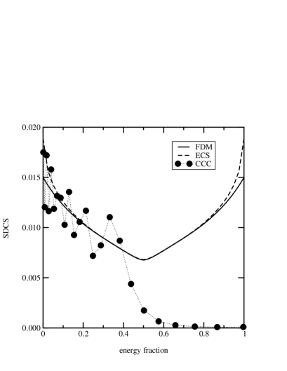
FIG. 1.: Singlet SDCS ($\pi a_{o}^{2}/{\rm Ryd}$) vs. the energy fraction $\epsilon_{b}/E$ for an impact energy of 54.4 eV. The total ionization cross sections from FDM, ECS, and CCC are $1.50^{-2}$,$1.54^{-2}$, and $1.48^{-2}$ ($\pi a_{o}^{2}$), respectively.

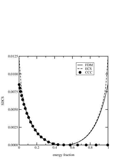
FIG. 2.: Same as Fig. 1 for the triplet case. The total ionization cross sections from FDM, ECS, and CCC are $3.11^{-3}$, $3.39^{-3}$, and $3.21^{-3}$ ($\pi a_{o}^{2}$), respectively.

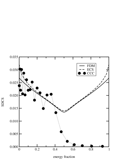
FIG. 3.: Singlet SDCS ($\pi a_{o}^{2}/{\rm Ryd}$) vs. the energy fraction $\epsilon_{b}/E$ for an impact energy of 40.8 eV. The total ionization cross sections from FDM, ECS, and CCC are $1.97^{-2}$, $2.04^{-2}$, and $2.02^{-2}$ ($\pi a_{o}^{2}$), respectively.

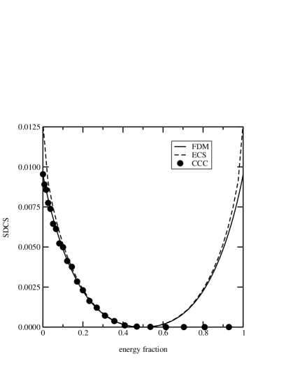
FIG. 4.: Same as Fig. 3 for the triplet case. The total ionization cross sections from FDM, ECS, and CCC are $2.47^{-3}$, $2.70^{-3}$, and $2.50^{-3}$ ($\pi a_{o}^{2}$), respectively.

In Figures 1-4, we present our results (labeled FDM for finite-difference method) for the single-differential cross section (SDCS). For a total energy of 3 Ryd, 240 a.u. proved to be a sufficient matching radius to get convergence of the SDCS and for E = 2 Ryd, a radius of 360 a.u. was required. The SDCS is more sensitive to the number of expansion functions for the continuum than the other observables, particularly about $\epsilon_{b}=E/2$. Nevertheless, convergence to better than 1% was readily obtained using 7-8 functions (the largest discrepancy in the SDCS between $N_{c}=7$ and $N_{c}=8$ was smaller than 0.3%; even using just 6 expansion function gave results accurate to 1%).

Also shown in Figs. 1-4 are the results of convergent close-coupling (CCC) calculations [3]. The CCC method of Bray [3] employs a “distinguishable electron” prescription, which produces energy distributions that are not symmetric about $\epsilon_{b}=E/2$. Stelbovics [8] has shown that a properly symmetrized CCC amplitude yields SDCS that are symmetric about $E/2$ as well as being four times larger at $\epsilon_{b}=E/2$ than those assuming distinguishable electrons. (Note that our singlet FDM results at $\epsilon_{b}=E/2$ are about four times larger than the corresponding CCC results.) Other than making the energy distributions symmetric, it is clear from the figures that symmetrization (coherent summation of the CCC amplitudes $C_{\epsilon_{b}i}$ and $C_{\epsilon_{a}i}$, where $\epsilon_{a}=E-\epsilon_{b}$, which correspond to physically indistinguishable processes) will significantly affect only singlet scattering (and then only near $\epsilon_{b}=E/2$), since $C_{\epsilon_{b}i}$ is practically zero for $\epsilon_{b}>E/2$. For singlet scattering, the CCC oscillates about the true value of SDCS, except near (and beyond) $\epsilon_{b}=E/2$. CCC results for triplet scattering, on the other hand, are in very good agreement with our results for $0\leq\epsilon_{b}\leq E/2$.

Some very recent results from Baertschy et al. [6] have also been included in the figures. Baertschy et al. rearrange the Schrödinger equation to solve for the outgoing scattered wave. They use a two-dimensional grid like ours, but scale the coordinates by a complex phase factor beyond a certain radius where the tail of the Coulomb potential is ignored. As a result, the scattered wave decays like an ordinary bound state beyond this cut-off radius, which makes the asymptotic boundary conditions very simple. By computing the outgoing flux directly from the scattered wave at several large cut-off radii, and extrapolating to infinity, they obtain the single-differential ionization cross section without having to use Coulomb three-body boundary conditions. This method, called exterior complex scaling (ECS), has just been extended to the full electron-hydrogen ionization problem [7]. It is seen from Figs. 1-4 that the ECS results are in good agreement with our FDM results except when the energy fraction $\epsilon_{b}/E$ approaches 0 or 1. Baertschy et al. [6] note that their method may be unreliable as $\epsilon_{b}$ approaches 0 or $E$ due to “contamination” of the ionization flux by contributions from discrete excitations.

We note also the recent work of Miyashita et al. [9], who have presented SDCS for total energies of 4, 2, and 0.1 Ryd using two different methods. One produces an asymmetric energy distribution similar to that of CCC while the other gives a symmetric distribution. Both contain oscillations. The mean of their symmetric curve at $E=2$ Ryd (40.8 eV impact energy) is in reasonable agreement with our calculations.

In conclusion, we have presented complete, precision results for the Temkin-Poet electron-hydrogen scattering problem for impact energies of 54.4 and 40.8 eV. It may be possible to improve the speed of the present method by using a variable-spaced grid, like that used by Botero and Shertzer [10] in their finite-element analysis (this would greatly reduce storage requirements as well). Once we have optimized our code for this simplified model we will proceed to include angular momentum. When angular momentum is included, the ionization boundary condition is no longer separable and this is the major challenge for generalizing the present approach to the full electron-hydrogen scattering problem.

The authors gratefully acknowledge the financial support of the Australian Research Council for this work.

REFERENCES

- [1] A. Temkin Phys. Rev. 126 130 (1962).
- [2] R. Poet, J. Phys. B 11, 3081 (1978).
- [3] I. Bray, Phys. Rev. Lett. 78, 4721 (1997).
- [4] R. Poet, J. Phys. B 13, 2995 (1980).
- [5] S. Jones and A. T. Stelbovics, Aust. J. Phys. (in press).
- [6] M. Baertschy, T. N. Rescigno, and C. W. McCurdy, Phys. Rev. A (in press).
- [7] M. Baertschy, T. N. Rescigno, and C. W. McCurdy, submitted to Phys. Rev. Lett.
- [8] A. T. Stelbovics, submitted to Phys. Rev. Lett.
- [9] N. Miyashita, D. Kato, and S. Watanabe, Phys. Rev. A (in press).
- [10] J. Botero and J. Shertzer, Phys. Rev. A 46, R1155 (1992).