Models for energy and charge transport
and storage in biomolecules

Abstract

Two models for energy and charge transport and storage in biomolecules are considered. A model based on the discrete nonlinear Schrödinger equation with long-range dispersive interactions (LRI’s) between base pairs of DNA is offered for the description of nonlinear dynamics of the DNA molecule. We show that LRI’s are responsible for the existence of an interval of bistability where two stable stationary states, a narrow, pinned state and a broad, mobile state, coexist at each value of the total energy. The possibility of controlled switching between pinned and mobile states is demonstrated. The mechanism could be important for controlling energy storage and transport in DNA molecules. Another model is offered for the description of nonlinear excitations in proteins and other anharmonic biomolecules. We show that in the highly anharmonic systems a bound state of Davydov and Boussinesq solitons can exist.

Key words:  bistability, long-range dispersion, bound state, anharmonic, nonlocal, soliton.

Published:  Journal of Biological Physics 25, 41–63 (1999).

I Introduction

Understanding how biological macromolecules (proteins, DNA, RNA, etc.) function in the living cells remains the major challenge in molecular biology. One of the most important questions is the mechanism of gene expression. The expression of a given gene involves two steps: transcription and translation. The transcription includes copying the linear genetic information into the messenger ribonucleic acid (mRNA). The information stored in mRNA is transferred into a sequence of aminoacids using the genetic code. mRNA is produced by the enzyme RNA-polymerase (RNAP) which binds to the promoter segment of DNA. As a result of the interaction between RNAP and promoter of DNA the so-called ”bubble” (i.e. a state in which 10–20 base pairs are disrupted) is formed. The disruption of 20 base pairs corresponds to investing some 100 kcal/mole (0.43 eV) [1].

In the framework of a linear model the large-amplitude motion of the bases was supposed to occur due to an interference mechanism [2]. According to this model energetic solvent molecules kick DNA and create elastic waves therein. As a result of the interference of two counter propagating elastic waves, the base displacements may exceed the elasticity threshold such that DNA undergoes a transition to a kink form which is more flexible. A similar approach was also proposed in Refs. [3, 4]. The linear elastic waves in DNA are assumed to be strong enough to break a hydrogen bond and thereby facilitate the disruption of base pairs. In spite of the attractiveness of this theory, which gives at least a qualitative interpretation of the experimental data [5], there are the following fundamental difficulties which to our opinion are inherent in the linear model of the DNA dynamics: (i) The dispersive properties (the dependence of the group velocity on the wave length) of the vibrational degrees of freedom in DNA will cause spreading of the wave packets and therefore smear the interference pattern. Furthermore, it has been shown [6] that the amplitudes of the sugar and the base vibrations are rather large even in a crystalline phase of DNA. Since the large-amplitude vibrations in the molecules and the molecular complexes are usually highly anharmonic their nonlinear properties can not be ignored; (ii) Molecules and ions which exist in the solution permanently interact with DNA. These interactions are usually considered as white noise and their influence is modelled by introducing Langevin stochastic forces into the equations describing the intramolecular motion. It is well known [7] that stochastic forces provide relaxation of linear excitations and destroy their coherent properties. Equivalently the coherence length (the length of the concerted motions) rapidly decreases with increasing temperature; (iii) DNA is a complex system which has many nearly isoenergetic ground states and may therefore be considered as a fluctuating aperiodic system. DNA may have physical characteristics in common with quasi-one-dimensional disordered crystals or glasses. However, it is known [8] that the transmission coefficient for a linear wave propagating in a disordered chain decreases exponentially with the growth of the distance (Anderson localization). In this way it is difficult to explain in the framework of linear theory such a phenomenon as an action at distance, where concerted motion initiated at one end of a biological molecule can be transmitted to its other end.

The above mentioned fundamental problems can be overcome in the framework of nonlinear models of DNA. Nonlinear interactions can give rise to very stable excitations, called solitons, which can travel without changing their shape. These excitations are very robust and important in the coherent transfer of energy [9]. For realistic interatomic potentials the solitary waves are compressive and supersonic. They propagate without energy loss, and their collisions are almost elastic.

Nonlinear interactions between atoms in DNA can give rise to intrinsically localized breather-like vibration modes [10, 11]. Such localized modes, being large-amplitude vibrations of a few (2 or 3) particles, can facilitate the disruption of base pairs and in this way initiate conformational transitions in DNA. These modes can occur as a result of modulational instability of continuum-like nonlinear modes [12], which is created by energy exchange mechanisms between the nonlinear excitations. The latter favors the growth of the large excitations [13].

Nonlinear solitary excitations can maintain their overall shape on long time scales even in the presence of the thermal fluctuations. Their robust character under the influence of white noise was demonstrated [14] and a simplified model of double-stranded DNA was proposed and explored. Quite recently the stability of highly localized, breather-like, excitations in discrete nonlinear lattices under the influence of thermal fluctuations was investigated [15]. It was shown that the lifetime of a breather increases with increasing nonlinearity, and in this way these intrinsically localized modes may provide an excitation energy storage even at room temperatures where the environment is strongly fluctuating.

Several theoretical models have been proposed in the study of the nonlinear dynamics and statistical mechanics of DNA (see the very comprehensive review [16]). A particularly fruitful model was proposed by Peyrard and Bishop [17] and Techera, Daemen and Prohofsky [18]. In the framework of this model the DNA molecule is considered to consist of two chains that are transversely coupled. Each chain models one of the two polynucleotide strands of the DNA molecule. A base is considered to be a rigid body connected with its opposite partner through the hydrogen-bond potential $V(u_{n})$, where $u_{n}$ is the stretching of the bond connecting the bases, $n$, and $n=0,\pm 1,\pm 2,..$ is labelling the base-pairs. The stretching of the $n^{\prime}$th base-pair is coupled with the stretching of the $m^{\prime}$th base-pair through a dispersive potential $U(u_{n},u_{m})$. The process of DNA denaturation was studied [17, 19] under the assumption that the coupling between neighboring base-pairs is harmonic $U(u_{n},u_{n+1})$. An entropy-driven denaturation was investigated [20] taking into account a nonlinear potential $U(u_{n},u_{n+1})$ between neighboring base-pairs. The Morse potential was chosen [17, 19, 20] as the on-site potential $V(u_{n})$, but also the longitudinal wave propagation and the denaturation of DNA has been investigated [14] using the Lennard-Jones potential to describe the hydrogen bonds.

In the main part of the previous studies the dispersive interaction $U$ was assumed to be short-ranged and a nearest-neighbor approximation was used. It is worth noticing, however, that one of two hydrogen bonds which is responsible for the interbase coupling, namely the hydrogen bond in the $N-H...O$ group, is characterized by a finite dipole moment. Therefore, a stretching of the base-pair will cause a change of the dipole moment, so that the excitation transfer in the molecule will be due to transition dipole-dipole interaction with a $1/r^{3}$ dependence on the distance, $r$. It is also well known that nucleotides in DNA are connected by hydrogen-bonded water filaments [21, 22]. In this case an effective long-range excitation transfer may occur due to the nucleotide-water coupling.

In the last few years the importance of the effect of long-range interactions (LRI) on the properties of nonlinear excitations was demonstrated in several different areas of physics [23, 24, 25, 26, 27, 28]. Quite recently [29], we proposed a new nonlocal discrete NLS model with a power dependence on the distance of the matrix element of the dispersive interaction. It was found that there is an interval of bistability in the NLS models with a long-range dispersive interaction. One of these states is a continuum-like soliton and the other is an intrinsically localized state.

Another model, which we consider in this paper, describes an excitation energy (or excess electron) transport in a highly anharmonic molecular chain. This line of investigation is rather new, since until recently most attention has been concentrated on strongly elastic systems, such as the excitons in the $\alpha$-helix proteins. The subsonic Davydov solitons can exist in this case, and the harmonic approximation is enough for a consideration of the lattice deformation caused by the exciton [30, 31]. But if the lattice is not supposed to be rigid or if the motion of the excitation at supersonic velocities is studied, the deformation cannot be considered small and anharmonic terms must be taken into account. For example, the anharmonic interactions play an important role in the dynamics of $DNA$. It is possible that they might concentrate vibrational energy in $DNA$ into soliton-like objects [14, 32].

The anharmonic Davydov model of the molecular chain has already been much studied during the last fifteen years [30, 33, 34, 35, 36, 37, 38, 39]. It is well known that there exist solitons of Davydov type and of Boussinesq type in the system. Pérez and Theodorakopoulos [40] investigated numerically an interaction between these solitons in the $\alpha$-helix proteins, and concluded that it inhibits the stability of the Davydov vibrational soliton at room temperature. But the effective anharmonicity parameter in that system is rather small. The recent investigations on the subject [36, 37, 38, 39] demonstrated that in highly anharmonic chains (e.g. in the problem of excess electron transfer in $\alpha$-helix proteins), the interaction between Davydov and Boussinesq solitons changes its sign, and the solitons can form a bound state.

The outline of the paper is the following. In Sec. II we investigate the effects of long-range interactions on the nonlinear dynamics of the two-strand model of DNA. First, we reduce the equations of motion of the model to the nonlocal discrete nonlinear Schrödinger (NLS) equation. Then, we present the analytical theory and the results of numerical simulations of the discrete NLS model with a long-range dispersive interaction. We obtain stationary localized solutions, demonstrate the existence of the bistability phenomenon, and discuss their stability. The investigation of the switching between bistable states completes the section. We show that a controlled switching between narrow, pinned states and broad, mobile states with only small radiative losses is possible when the stationary states possess an internal breathing mode. In Sec. III we investigate the anharmonic Davydov model of the molecular chain and show that it reduces to the Hénon - Heiles system [41], which is completely integrable at some fixed value of anharmonicity. There are three types of stationary solitons in this case: Boussinesq, Davydov, and a new type, namely a supersonic two-bell shaped soliton. We calculate the energies of the solitons. Then, we develop a variational approach for the non-integrable case. We show that in the case of highly anharmonic chains, the two-bell shaped soliton is an oscillating bound state of Davydov and Boussinesq solitons. This bound state is caused by the excitation (or electron) tunnelling in the effective two-well potential which is created by the exciton (electron) – phonon interaction and anharmonic terms in the lattice potential. On the contrary, at small anharmonicity Davydov and Boussinesq solitons repel each other, and the bound state cannot exist. Finally, we test the dynamical stability of the bound state at various values of anharmonicity numerically.

II Effects of long-range dispersion: bistability of localized excitations

A System and equations of motion

In this section we study the two-strand model of DNA which is described by the Lagrangian

$$L=T-U_{BP}-U_{LR}\;,$$ (1)

where

$$T=\frac{M}{2}\,\sum_{n}\left(\frac{du_{n}}{dt}\right)^{2}$$ (2)

is the kinetic energy and $M$ is the mass of the base-pair,

$$U_{BP}=\sum_{n}V(u_{n})$$ (3)

is the potential energy which describes an intrabase-pair interaction, and

$$U_{LR}=\frac{1}{4}\,\sum\!\!\!\!\!\!\sum_{n,m(n\neq m)}\!\!\!J_{n,m}(u_{m}-u_{n})^{2}$$ (4)

is the long-range dispersive interbase-pair interaction of the stretchings. In Eqs. (2)–(4) $n$ and $m$ are base-pair indices. The value $u_{n}=0$ of the base-pair stretching corresponds to the minimum of the intrabase-pair potential $V(u_{n})$. We investigate the model with the following power dependence on the distance (assuming that the lattice constant equals unity) of the matrix element of the base elastic coupling

$$J_{n,m}=\frac{J}{|n-m|^{s}}\;,$$ (5)

where the constant $J$ characterizes the strength of the coupling, and $s$ is a parameter being introduced to cover different physical situations including the nearest-neighbor approximation ($s=\infty$), quadrupole-quadrupole ($s=5$) and dipole-dipole ($s=3$) interactions. In the case of the DNA molecule the long-range interaction is evolved from the existence of charged groups in the DNA molecule. To take into account a possibility of screening of the interaction or an indirect coupling between base-pairs (e.g. via water filaments), we shall consider also the case when the matrix element of the base elastic coupling has the Kac-Baker [42, 43] form

$$J_{n,m}=J\,e^{-\beta|n-m|}\;,$$ (6)

where $\beta$ is the inverse radius of the interaction.

Assuming that

$$\left.\frac{\partial^{2}V(u_{n})}{\partial u_{n}^{2}}\right|_{u_{n}=0}\,\gg\,\left.\frac{\partial^{j}V(u_{n})}{\partial u_{n}^{j}}\right|_{u_{n}=0}$$ (7)

for $j=3,4,...$, that is the anharmonicity of the intrabase-pair potential is rather small, we shall use a rotating-wave approximation

$$u_{n}=\psi_{n}\,e^{-i\Omega\,t}+c.c.\;,$$ (8)

where $\left.\Omega=\sqrt{V^{\prime\prime}(u_{n})/M}\right|_{u_{n}=0}$ is the frequency of the harmonic oscillations and $\psi_{n}(t)$ is the complex amplitude which is supposed to vary slowly with time. Inserting Eq. (8) into Eqs. (1)–(4) and averaging with respect to the fast oscillations of the frequency $\Omega$, we conclude that the effective Lagrangian of the system can be represented in the form

$${\cal L}=\frac{i}{2}\sum_{n}\left(\dot{\psi}_{n}\psi^{*}_{n}-\dot{\psi}_{n}^{*}\psi_{n}\right)-{\cal H}\;,$$ (9)

where the dot denotes the differentiation with respect to the rescaled time $\tau=t/(2M\Omega)$. Here

$${\cal H}={\cal U}_{BP}+{\cal U}_{LR}\;$$ (10)

is the effective Hamiltonian of the system, where

$${\cal U}_{LR}=\frac{1}{2}\,\sum\!\!\!\!\!\!\sum_{n,m(n\neq m)}\!\!\!J_{n,m}|\psi_{m}-\psi_{n}|^{2}$$ (11)

is the effective dispersive energy and

$${\cal U}_{BP} = \sum_{n}\Biggl{(}\frac{\Omega}{2\pi}\int_{0}^{2\pi/\Omega}V(\psi_{n}\,e^{-i\Omega\,t}+c.c)dt$$ (12)

$$- M\Omega^{2}\,|\psi_{n}|^{2}\Biggr{)}$$ (13)

is the effective intrabase-pair potential. Usually either a Morse potential [17, 19] or a Lennard-Jones potential [14] is used to model the hydrogen bonds. With these potentials however it is very complicated to obtain any analytical results. Therefore, to gain insight into the problem we shall use a simplified nonlinear potential in the form

$${\cal U}_{BP}=-\frac{1}{(\sigma+1)}\sum_{n}|\psi_{n}|^{2(\sigma+1)}\;,$$ (14)

where the degree of nonlinearity $\sigma$ is a parameter which we include to have the possibility to tune the nonlinearity as well.

From the Hamiltonian (10) we obtain the equation of motion $i\dot{\psi_{n}}=\displaystyle{\frac{\partial{\cal H}}{\partial\psi_{n}^{*}}}$ for the wave function $\psi_{n}(\tau)$ in the form

$$i\dot{\psi_{n}}+\sum_{m(m\neq n)}J_{n,m}(\psi_{m}-\psi_{n})+|\psi_{n}|^{2\sigma}\psi_{n}=0\;.$$ (15)

The Hamiltonian ${\cal H}$ and the number of excitations

$$N=\sum_{n}|\psi_{n}|^{2}$$ (16)

are conserved quantities.

Thus we have reduced the equations of motion of the initial model of DNA dynamics to the nonlocal discrete nonlinear Schrödinger (NLS) equation studied quite recently in detail [29, 44]. In what follows we shall review the obtained results in application to the DNA molecule.

Looking for the stationary solutions of Eq. (15) of the form

$$\psi_{n}=\phi_{n}\exp(i\Lambda\tau)$$ (17)

with a real shape function $\phi_{n}$ and frequency $\Lambda$, we obtain the equation for $\phi_{n}$ in the form

$$\Lambda\phi_{n}=\sum_{m(m\neq n)}J_{n,m}(\phi_{m}-\phi_{n})+\phi_{n}^{(2\sigma+1)}$$ (18)

with $J_{n,m}$ described by Eqs. (5) or (6). Thus Eq. (18) is the Euler-Lagrange equation for the problem of extremizing ${\cal H}$ under the constraint $N=constant$.

B Bistability of stationary states

To develop a variational approach to the problem we use an ansatz for a localized state in the form

$$\phi_{n}=\sqrt{N\tanh\alpha}\exp(-\alpha|n|)\;,$$ (19)

where $\alpha$ is a trial parameter. This ansatz is chosen to satisfy automatically the normalization condition (16), so that the problem of extremizing ${\cal H}$ under the constraint $N=constant$ is reduced to the problem of solving the equation $\displaystyle{\frac{d{\cal H}}{d\alpha}=0}$.

Inserting the trial function (19) into the Hamiltonian given by Eqs. (10), (11), (14) and (5) and evaluating the discrete sums which enter in these equations (see [29] for details), we get the dispersive part of the Hamiltonian

$${\cal U}_{LR} = 2NJ\{\zeta(s)-\tanh(\alpha)F(e^{-\alpha},s-1)$$ (20)

$$- F(e^{-\alpha},s)\}\;$$ (21)

and the intrabase-pair potential

$${\cal U}_{BP} = -\frac{N^{\sigma+1}}{\sigma+1}\,f_{\sigma}\;,$$ (22)

$$\quad\mbox{with}\quad f_{\sigma} = \tanh^{\sigma+1}(\alpha)\,\coth[(\sigma+1)\alpha]\;,$$ (23)

where

$$\zeta(s)=\sum_{n=1}^{\infty}n^{-s}\quad\mbox{and}\quad F(z,s)=\sum_{n=1}^{\infty}(z^{n}/n^{s})$$ (24)

are Riemann’s zeta function and Jonqière’s function, respectively.

According to the variational principle we should satisfy the condition $\displaystyle{\frac{d{\cal H}}{d\alpha}=0}$ which yields

$$N^{\sigma}=2(\sigma+1)J\,(\tanh(\alpha) F(e^{-\alpha},s-2)$$ (25)

$$+\tanh^{2}(\alpha) F(e^{-\alpha},s-1) )\left(\frac{df_{\sigma}}{d\alpha}\right)^{-1}\;.$$ (26)

As a direct consequence of Eq. (18), the frequency $\Lambda$ can be expressed as

$$\Lambda=-\frac{1}{N}\,({\cal U}_{LR}+2\,{\cal U}_{BP})$$ (27)

with ${\cal U}_{LR}$ and ${\cal U}_{BP}$ being defined by Eqs. (21) and (23).

The results of the above developed variational approach are plotted in Figure 1, which shows the energy of the localized excitations as a function of $N$ and $s$ for the particular case $\sigma=1$.

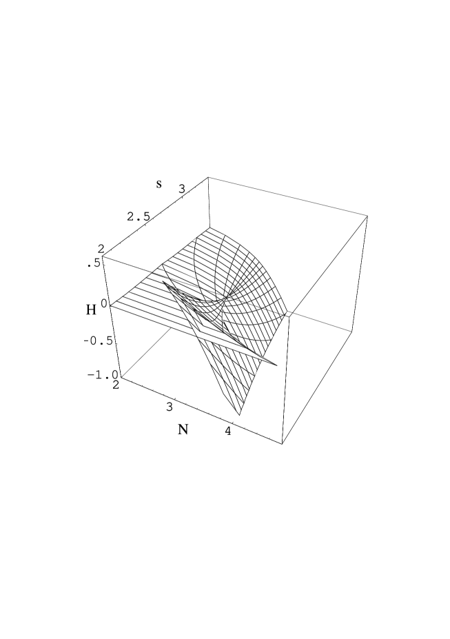
FIG. 1.: The dependence of the energy $H$ of stationary soliton solutions versus the excitation number $N$ and the dispersion parameter $s$, obtained from the variational approach for $\sigma=1$.

One can see that there is a critical value $s_{cr}=2.72$ of the dispersion parameter $s$ which separates two qualitatively different regions. The region $s>s_{cr}$ is characterized by the usual monotonic behavior of the soliton energy vs number of excitations $N$. Thus the main features of all discrete NLS models with dispersive interaction $J_{n,m}$ decreasing faster than $|n-m|^{-s_{cr}}$ coincide qualitatively with the features obtained in the nearest-neighbor approximation where only one stationary state exists for any $N$. But for $2<s<s_{cr}$ the bifurcation “swallow tail” takes place introducing a multistability into the system. One can see that in this case there is an energy interval where for each value of ${\cal H}$ there exist three stationary states with different excitation numbers. The direct numerical solution of Eq. (18) validates this conclusion and gives the precise critical value $s_{cr}=3.03$. It is noteworthy that similar results are obtained for the Kac-Baker dispersive interaction (6). In this case the multistability takes place for $\beta<1.70$.

FIG. 2.: Number of excitations, $N$, versus frequency, $\Lambda$, numerically from Eq. (18) for $\sigma=1$ and $s=\infty$ (full), 3 (dotted), 2.3 (dashed), 2 (short-long-dashed), and 1.9 (long-dashed).

FIG. 3.: Shapes of the three stationary states for $s=2.3$ and $N=3.2$. The stable: $\Lambda=0.11$ and $\Lambda=0.98$ (full). The unstable: $\Lambda=0.43$ (dashed).

Figure 2 shows the dependence $N(\Lambda)$ obtained numerically for $\sigma=1$. This dependence demonstrates the same transition from the monotonic behavior for $s>s_{cr}$ to the non-monotonic (${\cal N}$-type) behavior for $s<s_{cr}$ and assists to determine the stability of the stationary states. According to the theorem which was recently proven [45], the necessary and sufficient linear stability criterion for the stationary states is

$$\frac{dN}{d\Lambda}=\frac{d}{d\Lambda}\,\sum_{n}\,\phi_{n}^{2}>0\;.$$ (28)

Therefore we can conclude that only two stationary states are stable. The third state, with intermediate value of $\Lambda$ and maximal value of energy, is unstable. Thus it is reasonably to talk about bistability of the system.

The observed bistability is very similar to the one recently observed [45, 46], where the nearest-neighbor case with an arbitrary degree of nonlinearity $\sigma$ was studied. The bistability appears in this case for $\sigma$ above a certain critical value.

Figure 3 shows that the shapes of these solutions differ significantly. The low-frequency states are wide and continuum-like, while the high-frequency solutions represent intrinsically localized states with a width of a few lattice spacings.

Now we turn to discuss stationary states of the discrete NLS model given by Eq. (18) with arbitrary degree of nonlinearity. The main properties of the system remain unchanged, but the critical value $s_{cr}$ of the dispersion parameter is now a function of $\sigma$. The results of analytical consideration confirmed by simulation show that $s_{cr}$ increases with increasing $\sigma$. In particular, for $\sigma\geq 1.4$ (the value at which the discrete symmetrical ground state can be unstable in the nearest-neighbor approximation [45]) the bistability in the nonlinear energy spectrum occurs even for $s\leq 6$.

C Switching between bistable states

Having established the existence of bistable stationary states in the nonlocal discrete NLS system, a natural question that arises concerns the role of these states in the full dynamics of the model. In particular, it is of interest to investigate the possibility of switching between the stable states under the influence of external perturbations, and what type of perturbations that could be used to control the switching. Switching of this type is important in the description of nonlinear transport and storage of energy in biomolecules like the DNA, since a mobile continuum-like excitation can provide action at distance, while the switching to a discrete, pinned state can facilitate the structural changes of the DNA [5, 16].

An illustration of how the presence of an internal breathing mode can affect the dynamics of a slightly perturbed stable stationary state is given in Figures 4 and 5. To excite the breathing mode we apply a spatially symmetrical, localized perturbation, which we choose to conserve the number of excitations in order not to change the effective nonlinearity of the system. The simplest choice, which we have used in the simulations shown here, is to kick the central site $n_{0}$ of the system at $t=0$ by adding a parametric force term of the form $\theta\delta_{n,n_{0}}\delta(\tau)\psi_{n}(\tau)$ to the left-hand-side of Eq. (15). All details and a physical motivation of the appearance of such kind of parametric kick are described in Ref. [44]. As can be easily shown, this perturbation affects only the site $n_{0}$ at $\tau=0$, and results in a ’twist’ of the stationary state at this state with an angle $\theta$, i.e. $\psi_{n_{0}}(0)=\phi_{n_{0}}\,e^{i\theta}$. The immediate consequence of this kick is, as can been deduced from the form of Eq. (15), that $\displaystyle{\frac{d}{d\tau}}\left(|\psi_{n_{0}}|^{2}\right)$ will be positive (negative) when $\theta>0$ ( $\theta<0$). Thus, to obtain switching from the continuum-like state to the discrete state we choose $\theta>0$, while we choose $\theta<0$ when investigating switching in the opposite direction. We find that in a large part of the multistability regime there is a well-defined threshold value $\theta_{th}$, such that when the initial phase torsion is smaller than $\theta_{th}$, periodic, slowly decaying ’breather’ oscillations around the initial state will occur, while for strong enough kicks (phase torsions larger than $\theta_{th}$) the state switches into the other stable stationary state.

FIG. 4.: Switching from continuum-like to discrete state for the NLS model with the Kac-Baker long-range interactions (6) where $\beta=1$. The initial state $\phi_{n}$ has the frequency $\Lambda\simeq 0.310$ and $N=3.6$. We plot a time evolution of $|\psi_{n_{0}}(\tau)|^{2}$ when a phase torsion is applied to the center site with $\theta=0.261$ (lower curve) and $\theta=0.262$ (upper curve), respectively; inset shows time evolution of $|\psi_{n}(\tau)|^{2}$ for $\theta=0.262$.

FIG. 5.: Switching from discrete to continuum-like state for the NLS model with the Kac-Baker long-range interactions (6) where $\beta=1$. The initial state $\phi_{n}$ has the frequency $\Lambda\simeq 1.423$ and $N=3.6$. We plot a time evolution of $|\psi_{n_{0}}(\tau)|^{2}$ when a phase torsion is applied to the center site with $\theta=-0.490$ (upper curve) and $\theta=-0.491$ (lower curve), respectively; inset shows time evolution of $|\psi_{n}(\tau)|^{2}$ for $\theta=-0.491$.

It is worth remarking that the particular choice of perturbation is not important for the qualitative features of the switching, as long as there is a substantial overlap between the perturbation and the internal breathing mode. We also believe that the mechanism for switching described here can be applied for any multistable system where the instability is connected with a breathing mode. For example, we observed [47] a similar switching behavior in the nearest neighbor discrete NLS equation with a higher degree of nonlinearity $\sigma$, which is known [45] to exhibit multistability.

III Effects of anharmonicity: bound state of Davydov and Boussinesq solitons

A System and equations of motion

Let us consider in this section an excitation energy (or excess electron) transport in the anharmonic molecular chain. In Davydov’s coherent states approximation [30] the Hamiltonian of the system takes on the form

$$H = -J\sum_{n}\left[\psi_{n}^{*}(\psi_{n+1}+\psi_{n-1})-2|\psi_{n}|^{2}\right]$$ (32)

$$+\chi\sum_{n}|\psi_{n}|^{2}(\beta_{n+1}-\beta_{n-1})$$

$$+\frac{1}{2}\sum_{n}\Bigl{[}M\left(\frac{d\beta_{n}}{dt}\right)^{2}+\omega(\beta_{n+1}-\beta_{n})^{2}$$

$$-\frac{2}{3}\alpha\omega(\beta_{n+1}-\beta_{n})^{3}\Bigr{]}\;.$$

Here, $\psi_{n}(t)$ is the excitation wave function of the molecule at site $n$, $\beta_{n}(t)$ is the displacement of the $n$-th molecule from equilibrium, $J$ is the matrix element of the excitation transition, the constant $\chi$ characterizes the exciton - displacement interaction, $M$ is the mass of the molecule, and the parameters $\omega$ and $\alpha$ characterize the elasticity and the anharmonicity of the lattice, respectively.

The equations of motion for $\psi_{n}(t)$ and $\beta_{n}(t)$ are

$$i\hbar\frac{d}{dt}\psi_{n}(t) = -J(\psi_{n+1}+\psi_{n-1}-2\psi_{n})$$ (34)

$$+\chi(\beta_{n+1}-\beta_{n-1})\psi_{n}\;,$$

$$M\frac{d^{2}}{dt^{2}}\beta_{n}(t) = \omega(\beta_{n+1}+\beta_{n-1}-2\beta_{n})$$ (36)

$$\times(1-\alpha(\beta_{n+1}-\beta_{n-1}))$$

$$+ \chi(|\psi_{n+1}|^{2}-|\psi_{n-1}|^{2})\;.$$ (37)

The Hamiltonian (32) conserves the number of excitations in the chain. We shall assume that there is only one excitation. Thus the normalization condition for the wave function $\psi_{n}(t)$ is

$$\sum_{n}|\psi_{n}(t)|^{2}=1\;.$$ (38)

Using the continuum limit $\psi_{n}(t)\to e^{ikx}\psi(x,t)$ and $\beta_{n}(t)\to\beta(x,t)$, where $x=n\ell$ and $\ell$ is the lattice constant, we shall consider the solutions in the form of travelling waves

$$\psi(x,t)=(8\Delta)^{-1/2}\;e^{i\Lambda t}\;\varphi(\vartheta)\;,$$ (39)

$$\partial\beta/\partial x=-(J\cos(k\ell)/\chi)\;u(\vartheta)\;,$$ (40)

where $\Delta=3\chi^{2}/(\omega J\cos(k\ell))$ and $\vartheta=(x-vt)/\ell$. As a result we obtain the system of equations

$$\ddot{\varphi}-A\varphi+2u\varphi=0\;,$$ (41)

$$\displaystyle{\frac{d^{2}}{d\vartheta^{2}}}(\ddot{u}-4Bu+gu^{2}-\varphi^{2})=0\;,$$ (42)

where the parameters $A$ , $B$ and $g$ are given by the expressions

$$A = (2J+\hbar\Lambda)/(J\cos(k\ell))-2\;,$$ (43)

$$B = 3(v^{2}/v_{0}^{2}-1)\;,$$ (44)

$$g = (12\alpha J\cos(k\ell))/\chi\;.$$ (45)

Here $v_{0}=\ell\sqrt{\omega/M}$ is the sound velocity, $v=(2J\ell/\hbar)\sin(k\ell)$ is the soliton velocity, and the dots denote the differentiation with respect to $\vartheta$ . We shall assume that the effective mass of excitation is positive, i.e. $J>0$, and consider the carrier wave vector $k$ in the interval $0\leq k\ell<\pi/2$.

At the boundary conditions

$u(\pm\infty)=\dot{u}(\pm\infty)=\ddot{u}(\pm\infty)=\varphi(\pm\infty)=\dot{\varphi}(\pm\infty)=0\;,$

the equations of motion (41) and (42) are similar to that of the Hénon-Heiles system [41] except for the sign in front to $\varphi^{2}$ in Eq. (42). This similarity has been used in our investigations [35, 36, 39] of the system — we shall review the results in what follows. An alternative approach to the problem has been developed recently by Zolotaryuk, Spatschek, and Savin [37, 38].

B The soliton solutions in the completely integrable case

It is well known that in a general case the Hénon-Heiles system [41] is not completely integrable. However in the following three cases [48]:

(i) $A=4B$ , $g=1$ ,
(ii) $4A=B$ , $g=16$ ,
(iii) $g=6$ and arbitrary $A$ and $B$ ,

there exists a second integral of motion, and thus it is a Liouville completely integrable system. The conditions (i) and (ii) can be satisfied for only one value of the soliton velocity, since the normalization condition (38) imposes a link between parameters $A$ and $B$. But we intend to investigate how the soliton energy and shape depend on the soliton velocity. Therefore we shall consider here only the third case. It was shown in Refs. [35, 36] that in this case there exist only three types of soliton solutions of Eqs. (41) and (42), namely:

(a) The Boussinesq soliton:

$$\varphi=0\;\;,\;\;\;\;\;\;u=\frac{6}{g}B\,\mbox{sech}^{2}\sqrt{B}\vartheta\;.$$ (46)

It exists at supersonic velocities for any $g$, and represents a lattice compression which moves along the chain without changing its shape.

(b) The Davydov soliton [33]:

$$\varphi=2\sqrt{A(A-B)}\,\mbox{sech}\sqrt{A}\vartheta\;\;,\;\;\;\;\;u=A\,\mbox{sech}^{2}\sqrt{A}\vartheta\;.$$ (47)

It exists at subsonic ($B<0$) as well as at supersonic ($B>0$) velocities, but only for $g=6$.

(c) The two-bell shaped soliton, which exists only at supersonic ($B>0$) velocities and $g=6$:

$$\varphi = 2\sqrt{A}(A-B)S^{-1}(\vartheta,R)\cosh\sqrt{B}(\vartheta-R)\;,$$ (48)

$$u = \frac{d^{2}}{d\vartheta^{2}}\ln S(\vartheta,R)\;,$$ (49)

where $R$ is an integration constant and

$$S(\vartheta,R) = \sqrt{A}\cosh(\sqrt{B}(\vartheta-R))\cosh(\sqrt{A}\vartheta)$$ (50)

$$- \sqrt{B}\sinh(\sqrt{B}(\vartheta-R))\sinh(\sqrt{A}\vartheta)\;.$$ (51)

This solution was found analytically and studied numerically in Refs. [35, 36], where it was interpreted as a bound state of Davydov and Boussinesq solitons. It was also found numerically in Refs. [37, 38] where the authors believe, in contrast to our conclusion, that it is a bound state of a Davydov soliton with two Boussinesq solitons.

It is interesting to note that the deformation function (50) has the form of the two-soliton solution of the KdV–equation [49]. So we can conclude that the excitation $\varphi(\vartheta)$ is similar to that of a quantum particle moving in two-well potential $-2u(\vartheta)$ (see Figure 6). One of the wells is created by the lattice soliton, and the second is caused by the interaction of the excitation with the lattice. Part of the time the particle lives in the well that was dug by itself, then it tunnels to the well that was created by the lattice soliton, and so on. As a result of such a complicated behavior we obtain a wave function $\varphi(\vartheta)\;$ in the form of Eq. (49) (see Figure 6). It is interesting to remark that at the velocity within the range

$$v_{0}<v<v_{0}[1+(\Delta^{2}/54)^{1/3}]^{1/2}\;,$$ (52)

the wave function of the soliton has the one-bell shape at any distance $R$ between the wells in the potential $-2u(\vartheta)$. On the contrary, if the velocity exceeds $v_{0}[1+(\Delta/2)^{2/3}]^{1/2}$ we obtain the two-bell shape at any $R$. However, the ratio of the soliton maximal values in this case is proportional to $\mbox{sech}\sqrt{A}R$ at $|R|\gg 1/\sqrt{B}$. Thus we may conclude that the excitation (or electron) lives mostly in the well that was dug out by itself, tunnelling to the other well with an exponentially small rate.

FIG. 6.: The form of the two-bell shaped solitons at $\Delta=1$ and $v=1.2v_{0}$ for different values of distance $R$: $R=0$ (solid), $R=1$ (dashed), and $R=6$ (dotted).

We have calculated (see Figure 7) the velocity dependence of the soliton energy for all three types of solitons at $g=6$. For the energy of Boussinesq soliton (46) we get

$$E_{Bq}=\frac{2\omega}{3}\left(1+\frac{4}{15}B\right)B^{3/2}\;.$$ (53)

The energy of Davydov soliton (47) is given by the expression

$$E_{Dav}=E_{ex}+J\cos(k\ell)\left[\frac{2}{5\Delta}\left(1+4\frac{v^{2}}{v_{0}^{2}}\right)A^{3/2}-\frac{3}{10}A\right]\;,$$ (54)

where

$$E_{ex}=\frac{\hbar^{2}v^{2}}{8J\ell^{2}}\cos(k\ell)\;$$ (55)

is the exciton energy and $A$ is determined by the equation

$$\sqrt{A}(A-B)=\Delta\;.$$ (56)

Finally the energy of the two-bell shaped soliton turned out to be an exact sum of the energies of the Davydov and Boussinesq solitons:

$$E_{II}=E_{Dav}+E_{Bq}\;.$$ (57)

It is interesting that this energy does not depend on the distance $R$. It means that at $g=6$ the Davydov and Boussinesq solitons do not interact. However, as it will be shown below they interact in the non-integrable case $g\neq 6$. Namely, they repel each other at $g<6$ and form a bound state at $g>6$.

FIG. 7.: The energy of the Davydov ($E_{Dav}$), Boussinesq ($E_{Bq}$) and two-bell shaped ($E_{II}$) solitons vs the velocity, for $\Delta=10$.

C Variational approach in the non-integrable case

In what follows we shall develop a variational approach to the investigation of the behavior of the two-bell shaped solitons in the anharmonic chain far from the completely integrable case. Considering the Hamiltonian (32), one can see that the Lagrangian of the chain has the form

$$L =\sum_{n}\frac{i\hbar}{2}[\psi_{n}^{*}\partial_{t}\psi_{n}-\psi_{n}\partial_{t}\psi_{n}^{*}]$$ (62)

$$+\sum_{n}\psi_{n}^{*}[J(\psi_{n+1}+\psi_{n-1}-2\psi_{n})$$

$$-\chi(\beta_{n+1}-\beta_{n-1})\psi_{n}]$$

$$+\frac{M}{2}\sum_{n}(\partial_{t}\beta_{n})^{2}$$

$$-\frac{\omega}{2}\sum_{n}\left[(\beta_{n+1}-\beta_{n})^{2}-\frac{2\alpha}{3}(\beta_{n+1}-\beta_{n})^{3}\right]\;.$$

Substituting into it the solution (49) of Eqs. (41) and (42) as a trial function ($A$ and $B$ are supposed to be constant and $R$ is time dependent), we obtain an effective Lagrangian $L(R,\partial_{t}R)$. If the soliton velocity is close to the sound velocity ($B\ll A$) the energy of the two-bell shaped soliton is

$$E_{II}\simeq E_{Dav}+E_{Bq}+J\cos(k\ell)\frac{B^{3/2}}{\Delta}\left(\frac{dR}{d\tau}\right)^{2}$$ (63)

$$+J\cos(k\ell)\frac{g-6}{18}\left[\frac{4}{5}\Delta^{2/3}+B\{4-\mbox{sech}^{2}(\sqrt{B}R)\}\right]\;.$$ (64)

The equation of motion in this case is

$$\frac{d^{2}R}{d\tau^{2}}+\frac{\nu^{2}}{\sqrt{B}}\frac{\sinh(\sqrt{B}R)}{\cosh^{3}(\sqrt{B}R)}=0\;,$$ (65)

where $\nu^{2}=(g-6)\sqrt{B}\Delta/18$ and $\tau=\sqrt{\omega/M}\,t$ is the dimensionless time.

One can see that at $g<6$ there is an intersoliton repulsion. The distance $R\to\infty$ when $\tau\to\infty$, and the two-bell shaped soliton is dissociated into Davydov and Boussinesq solitons.

On the contrary, at $g>6$ there is a potential well in Eq. (63), and the distance $R$ between solitons is a periodic function

$$\sinh(\sqrt{B}R)=\sinh(\sqrt{B}R_{0})\sin\frac{2\pi}{T}(\tau-\tau_{0})\;,$$ (66)

with the period of oscillations

$$T=\frac{2\pi}{\nu}\cosh(\sqrt{B}R_{0})\;.$$ (67)

Here $R_{0}$ is the maximum value of $R$ and $\tau_{0}$ is the initial time.

FIG. 8.: Numerical calculations of the dynamics of two-bell shaped solitons for $g=8.5$ at different moments of dimensionless time: (a) $\tau=0$, (b) $\tau=1550$, (c) $\tau=3510$, (d) $\tau=5400$, (e) $\tau=6460$. The boundary conditions are periodic.

Thus, we can conclude that in highly anharmonic molecular chains, there should exist a bound state of Davydov and Boussinesq solitons. The dynamical stability of this bound state has been tested numerically. In Figure 8 we present the results of numerical simulations for $g=8.5$. As an initial state we chose an asymmetric two-bell shaped soliton. One can see that as time increases, the bells approach each other and their heights (as well as the depths of wells) equalize. Thereafter, the distance between the bells increases, and a mirror reflected asymmetric two-bell shaped soliton appears. Thus, the Davydov and Boussinesq solitons form a rather stable bound state and demonstrate an oscillating motion in accordance with Eq. (66).

In conclusion, we note that for the Davydov vibrational soliton motion in the $\alpha$–helix molecule the parameter $g\simeq 0.8$, so that the bound state of supersonic Davydov and Boussinesq soliton cannot exist. But for the electron motion in the polypeptide molecule we get $g\geq 12$. Thus we arrive at the conclusion that the bound state of the supersonic Davydov electrosoliton and the Boussinesq soliton can exist in the $\alpha$–helix biopolymers.

IV Conclusion

We have considered two models for energy and charge transport and storage in biomolecules. In these models we took into account the long-range dispersive (first model) and anharmonic (second model) interactions, and showed that these interactions are responsible for the existence of new types of excitations.

We have proposed a new nonlocal discrete nonlinear Schrödinger (NLS) model for the modelling of the nonlinear dynamics of the DNA molecule with long-range ($r^{-s}$ and $e^{-\beta r}$) dispersive interaction between its charged groups. We have shown that when the long-range interactions decay slowly, there is an energy interval where two stable stationary states exist at each value of the Hamiltonian ${\cal H}$. One of these states is a continuum-like soliton and the other one is an intrinsically localized mode. By this means a bistability phenomenon came into existence in the system. This phenomenon is a result of the competition of two length scales: the usual scale of the NLS model, which is related to the competition between nonlinearity and dispersion (expressed in terms of the ratio $N/J$), and the radius of the long-range interactions.

We have shown that a controlled switching between narrow (pinned) states and broad (mobile) states is possible. Applying a perturbation in the form of a parametric kick, we demonstrated that switching occurs beyond some well-defined threshold value of the kick strength. The particular choice of perturbation is not important for the qualitative features of the switching, as long as there is a substantial overlap between the perturbation and the internal breathing mode. Thus, we believe that the mechanism for switching described here can be applied for any multistable system where the instability is connected with a breathing mode. The switching phenomenon could be important for controlling energy storage and transport in DNA molecules.

The second model is proposed for modelling of anharmonic biological macromolecules. We have shown that when the value of the effective (dimensionless) anharmonicity parameter is large enough, a bound state of Davydov and Boussinesq solitons can exist. For the Davydov vibrational soliton motion in the $\alpha$–helix proteins the anharmonicity parameter is too small, so that the bound state cannot exist. But for the excess electron motion in the polypeptide molecule it is rather large, and a bound state of the supersonic Davydov electrosoliton and the Boussinesq soliton can be formed. Furthermore, a slightly generalized version of the $DNA$ model [14] which takes into account next neighbors transversal interactions between Toda chains actually yields strong anharmonicity. Hence there is a wide range of values for the anharmonicity parameter $g$ occurring in real systems.

REFERENCES

- [1] Reiss, C., in M. Peyrard (ed.) Nonlinear Excitations in Biomolecules, Springer-Verlag, Berlin, Heidelberg, Les Editions de Physique Les Ulis, 1995, p.29.
- [2] Lozansky et al, in R.H. Sarma (ed.) Stereodynamics of Molecular Systems, Pergamon Press, 1979, p.265.
- [3] Chou, K.C. and Mao, B., Biopolymers, 27 (1988), 1795.
- [4] Prohovsky, E.W., in R.H. Sarma and M.H. Sarma (eds.) Biomolecular Stereodynamics IV, Adenine Guilderland, New York, 1986, p.21.
- [5] Georghiou et al, Biophysical J., 70 (1996), 1909.
- [6] Holbrook, S.R. and Kim, S.H., J. Mol. Biol., 173 (1984), 361.
- [7] Gaididei, Yu.B. and Serikov, A.A., Theor. and Math. Phys., 27 (1976), 457.
- [8] Papanicolaou, G.C., J. Appl. Math., 21 (1971), 13.
- [9] Wadati, M., J. Phys. Soc. Jpn., 38 (1976), 673.
- [10] Sievers, A.J. and Takeno, S., Phys. Rev. Lett., 61 (1988), 970.
- [11] MacKay, R.S. and Aubry, S., Nonlinearity, 7 (1994), 1623.
- [12] Pouget, J. et al, Phys. Rev. B, 47 (1993), 14866.
- [13] Dauxois, T. and Peyrard, M., Phys. Rev. Lett., 70 (1993), 3935.
- [14] Muto, V. et al, Phys. Rev. A, 42 (1990), 7452.
- [15] Christiansen, P.L. et al, Phys. Rev. B, 55 (1997), 5759.
- [16] Gaeta, G. et al, Riv. N. Chim., 17 (4) (1994), 1.
- [17] Peyrard, M. and Bishop, A., Phys. Rev. Lett., 62 (1989), 2755.
- [18] Techera, M. et al, Phys. Rev. A, 40 (1989), 6636.
- [19] Dauxois, T. et al, Phys. Rev. E, 47 (1993), 684.
- [20] Dauxois, T. et al, Phys. Rev. E, 47 (1993), R44.
- [21] Dahlborg, U. and Rupprecht, A., Biopolymers, 10 (1971), 849.
- [22] Corongiu, G. and Clementi, E., Biopolymers, 20 (1981), 551.
- [23] Braun, O.M. et al, Phys. Rev. B, 41 (1990), 7118.
- [24] Woafo, P. et al, J. Phys. Condens. Matter, 5 (1993), L123.
- [25] Vazquez, L. et al, Phys. Lett. A, 189 (1994), 454.
- [26] Alfimov, G.L et al, Chaos, 3 (1993), 405.
-
[27]
Gaididei, Yu.B. et al, Phys. Lett. A
222 (1996), 152;
Gaididei, Yu.B. et al, Phys. Scr. T67 (1996), 151. - [28] Gaididei, Yu.B. et al, Phys. Rev. Lett., 75 (1995), 2240.
- [29] Gaididei, Yu.B. et al, Phys. Rev. E, 55 (1997), 6141.
- [30] Davydov, A.S.: Solitons in molecular systems, D. Reidel Pub. Co., Dordrecht, Boston, Lancaster, 1987.
- [31] Christiansen, P.L. and Scott, A.C. (eds.): Davydov’s soliton revisited, NATO ASI Series B: Physics Vol. 243, Plenum Press, 1990.
- [32] Christiansen, P.L. et al, Chaos, Solitons and Fractals, 2 (1992), 45.
- [33] Davydov, A.S. and Zolotariuk, A.V. Phys. Stat. Sol. (b), 115 (1983), 115.
- [34] Davydov, A.S. and Zolotariuk, A.V., Phys. Scr., 30 (1984), 426.
- [35] Christiansen, P.L. et al, Phys. Lett. A, 166 (1992), 129.
- [36] Gaididei, Yu.B. et al, Phys. Scr., 51 (1995), 289.
- [37] Zolotaryuk, A.V. et al, Europhys. Lett., 31 (1995), 531.
- [38] Zolotaryuk, A.V. et al, Phys. Rev. B, 54 (1996), 266.
- [39] Mingaleev, S.F., Effects of Nonlocality and Anharmonicity in Nonlinear transport of energy and charge, Ph.D. thesis, (Kiev, 1997).
- [40] Pérez, P. and Theodorakopoulos, N., Phys. Lett. A, 124 (1987), 267.
- [41] Hénon, M. and Heiles, C., Astrophysics, 63 (1964), 73.
- [42] Baker, G.A. Jr, Phys. Rev., 122 (1961), 1477.
- [43] Kac, A.M. and Helfand, B.C., J. Math. Phys., 4 (1972), 1078.
- [44] Johansson, M. et al, Phys. Rev. E, 57 (1998), 4739.
- [45] Laedke, E.W. et al, Phys. Rev. Lett., 73 (1994), 1055.
- [46] Malomed, B. and Weinstein, M.I., Phys. Lett. A, 220 (1996), 91.
- [47] Johansson, M. et al, Physica D, 119 (1998), 115.
- [48] Lichtenberg, A.J. and Lieberman, M.A.: Regular and Stochastic motion, Springer-Verlag, Berlin, Heidelberg, New York, 1983.
- [49] Lamb, G.L. Jr.: Elements of Soliton Theory, John Wiley and Sons, New York, 1980.