A Piecewise-Conserved Constant of Motion for a Dissipative System

Abstract

We discuss a piecewise-conserved constant of motion for a simple dissipative oscillatory mechanical system. The system is a harmonic oscillator with sliding (dry) friction. The piecewise-conserved constant of motion corresponds to the time average of the energy of the system during one half-period of the motion, and changes abruptly at the turning points of the motion. At late times the piecewise-conserved constant of motion degenerates to a constant of motion in the usual sense.

I Introduction

Finding constants of motion is an important step in the solution of many problems of Physics, as they allow to reduce the number of the degrees of freedom of the problem. Constants of motion are intimately related to conservation laws or symmetries of the system. For example, it is well known that a symmetry of the Lagrangian of a system is responsible, by virtue of Noether’s theorem, to a constant of motion [1]. By definition, a constant of motion preserves its value during the evolution of the system. Even in cases where there are no constants of motion, one could still sometimes find adiabatic invariants, which generalise the concept of a constant of motion to systems with slowly-varying parameters. It turns out, however, that there are cases where there are constants of motion, which are only piecewise-conserved. Well-known examples of such piecewise-conserved constants of motion arise from the generalisation of the Laplace-Runge-Lenz vector for general central potentials. For example, in the case of the three-dimensional isotropic harmonic oscillator, the Fradkin vector [2] (which generalises the Laplace-Runge-Lenz vector) abruptly reverses its direction (although preserves its magnitude) during a full period [3] (see also [4]). (The Fradkin vector directs toward the perigee, and the position of the perigee jumps discontinuously whenever the particle passes through the apogee.) Also, in the truncated Kepler problem, the Peres-Serebrennikov-Shabad vector abruptly changes its direction whenever the particle in motion passes through the periastron [5, 6]. Again, it is just the direction of the conserved vector which is only piecewise-conserved: the magnitude of the vector remains a constant of motion in the original meaning (namely, the magnitude has a fixed value throughout the motion). Piecewise-conserved constants of motion may also be relevant for systems which involve radiation reaction. In the above examples, the piecewise-conserved constants of motion appear in non-dissipative systems, and result from a discontinuity of the force (as in the truncated Kepler problem) or from geometrical considerations (as in the three-dimensional isotropic harmonic oscillator case). These piecewise-conserved constants of motion involve vectors rather than scalars, which still conserve their magnitude.

The following question arises: Can one find, for elementary systems, piecewise-conserved constants of motion? In what follows, we shall discuss an elementary piecewise-conserved scalar constant of motion, for a simple oscillatory mechanical model which involves dissipation in the form of sliding (dry) friction. Although dry friction is more nearly descriptive of everyday macroscopic motion in inviscid media, it is usually ignored in elementary mechanics courses and textbooks, which very frequently discuss viscous friction (which is velocity dependent). Dry friction exhibits, however, some very interesting features and can be readily presented in the laboratory or classroom demonstration.

The problem of a harmonic oscillator damped by dry friction was considered by several authors. Lapidus analised this problem for equal coefficients of static and kinetic friction, and found the position where the oscillator comes to rest [7]. Hudson and Finfgeld were able to find the general solution of the equation of motion [8]. However, they again assumed equal coefficients of static and kinetic friction, and used the Laplace transform technique, which is unknown to students of elementary mechanics courses, to generate the solution. An elementary solution, which ignores static friction, was derived by Barratt and Strobel [9]. This solution is based on solving separately for each half cycle of the motion, and is consequently tedious and unappealing. Recently, Zonetti et al. [10] considered the related problem of both dry and viscous friction for a pendulum, but did not offer a full analytic solution for the motion.

In this work, we find the general solution for the motion taking into account both static and kinetic friction, using elementary techniques which are available for students of elementary courses of mechanics. We analyse the solution using a piece-wise conserved constant of motion. The discussion, as well as the corresponding laboratory experiment of classroom demonstration, are suitable for a basic course for physics or engineering students.

II Elementary Discussion

Let a block of mass $M$ be placed on a horizontal surface, such that the coefficients of static and kinetic friction are $\mu_{s}$ and $\mu_{k}$, respectively. The block is attached to a linear spring with spring constant $k$ (for both compression and extension), such that initially the spring is stretched from its equilibrium length by $\ell$, and the block is kept at rest at $x=\ell$. At time $t=0$ the block is released. If $k\ell>\mu_{s}Mg$, $g$ being the gravitational acceleration, the block would start to accelerate. We take the friction to be small, namely $\mu_{s,k}\ll\ell k/(Mg)$, and also assume slow motion, such that the friction force is independent of the speed. Namely, we neglect effects such as air-resistance, and include only the force which results from the block touching the surface. We also neglect any variation of $\mu_{k}$ with the speed.

Immediately after the block starts accelerating, its motion is governed by the equation of motion

$$M\ddot{x}=-kx+\mu_{k}Mg,$$ (1)

with initial conditions $x(0)=\ell$ and $\dot{x}(0)=0$. From now on, let us introduce the frequency $\omega^{2}=k/M$. Of course, the system does not preserve its energy, due to the friction force. However, let us define a new coordinate $x^{\prime}=x-\mu_{k}g/\omega^{2}$. Equation (1) then becomes $\ddot{x^{\prime}}+\omega^{2}x^{\prime}=0$. For this equation we know that there is a constant of motion, namely ${\cal E}=\frac{1}{2}M\dot{x^{\prime}}^{2}+\frac{1}{2}M\omega^{2}x^{\prime 2}$. Therefore, despite the presence of friction, one can still find a constant of motion, which has the functional form of the total mechanical energy, but which is of course not the energy, as the latter is not conserved. Calculating its numerical value we find that ${\cal E}_{0}=\frac{1}{2}M\omega^{2}\left(\ell-\mu_{k}g/\omega^{2}\right)^{2}$.

At the time $t=\pi/\omega$ the velocity of the block vanishes, and it can be easily shown that at $t=\pi/\omega$ its acceleration is $\ddot{x}(\pi/\omega)=(\ell-\mu_{k}g/\omega^{2})\omega^{2}>0$, such that the block reverses its motion. (We assume here that $M\ddot{x}(\pi/\omega)>\mu_{s}Mg$.) The nature of the friction force is that its direction is always opposite to the direction of motion. Consequently, the equation of motion now changes to

$$M\ddot{x}=-kx-\mu_{k}Mg,$$ (2)

with initial conditions $x(\pi/\omega)=\ell-2\mu_{k}g/\omega^{2}$ and $\dot{x}(\pi/\omega)=0$. One can again solve this equation readily. This time, let us define $x^{\prime}=x+\mu_{k}g/\omega^{2}$. Equation (2) again becomes $\ddot{x^{\prime}}+\omega^{2}x^{\prime}=0$, such that ${\cal E}$ is still conserved. However, this time the numerical value of ${\cal E}$, which we denote by ${\cal E}_{1}\neq{\cal E}_{0}$, and we find ${\cal E}_{1}=\frac{1}{2}M\omega^{2}\left(\ell-3\mu_{k}g/\omega^{2}\right)^{2}$. One can describe the next phases of the motion similarly. During each phase of the motion (during half a period between two times at which the velocity vanishes) ${\cal E}$, if defined properly, is conserved. However, ${\cal E}$ is only piecewise-conserved, as its value changes abruptly from phase to phase. We note that the period of the oscillations is not altered by the presence of friction, and denote by $P_{1/2}$ half that period. Namely, $P_{1/2}\equiv\pi/\omega$.

III General Discussion

Let us now discuss the system in a more general way. It turns out that although there are friction forces, one can still write a hamiltonian

$$H(x,p;t)=\frac{1}{2M}p^{2}+\frac{1}{2}M\omega^{2}x^{2}-f(t)x,$$

where $f(t)=(-1)^{\left[t/P_{1/2}\right]}\mu_{k}Mg$. The equation of motion is now

$$\ddot{x}+\omega^{2}x=f(t)/M$$ (3)

with the initial conditions being (as before) $x(0)=\ell$ and $\dot{x}(0)=0$. We denote by square brackets of some argument the largest integer smaller than or equal to the argument. We also assume that the static friction force at the turning points of the motion is smaller than the elastic force of the spring, such that the motion does not stop. (Of course, for large enough time, this would not be true any more, and the block would eventually stop—see below.) Let us define the (complex) variable $\xi\equiv\dot{x}+i\omega x$ [11], where $i^{2}=-1$. Then, instead of a real second order equation (such as Eq. (3)), one obtains a complex first order equation. It is advantageous to do this, because there is a general solution for any inhomogeneous linear first-order differential equation in terms of quadratures. Substituting the definition for $\xi$ in Eq. (3) we find that the equation of motion, in terms of $\xi$, takes the form

$$\dot{\xi}-i\omega\xi=f(t)/M,$$ (4)

with the initial condition $\xi_{0}\equiv\xi(t=0)=i\omega\ell$. The solution of the equation of motion (4) is

$$\xi(t)=e^{i\omega t}\left\{\int_{0}^{t}\frac{1}{M}f(t^{\prime})e^{-i\omega t^{\prime}}\,dt^{\prime}+\xi_{0}\right\}.$$ (5)

After finding the solution $\xi(t)$ we can find $x(t)$ and $\dot{x}(t)$ by $\dot{x}(t)=(\xi(t)+\xi^{*}(t))/2$ and $x(t)=(\xi(t)-\xi^{*}(t))/(2i)$. We denote by a star complex conjugation. In order to integrate Eq. (5) we find it convenient to separate the discussion to two cases: case (a) where $\left[t/P_{1/2}\right]$ is an odd number (namely, $\left[t/P_{1/2}\right]=2n-1$), and case (b) where $\left[t/P_{1/2}\right]$ is even (namely, $\left[t/P_{1/2}\right]=2n$), where $n$ is integer. We next split the interval of integration in Eq. (5) into two parts: we first integrate from $t^{\prime}=0$ until $t_{2n-1}\equiv(2n-1)P_{1/2}$, and then integrate from $t_{2n-1}$ to $t$, and sum the two contributions. Integrating term by term we find

$$\int_{0}^{t_{2n-1}}\frac{1}{M}f(t^{\prime})e^{-i\omega t^{\prime}}\,dt^{\prime} = \sum_{j=0}^{n-1}\int_{2jP_{1/2}}^{(2j+1)P_{1/2}}\mu_{k}ge^{-i\omega t^{\prime}}\,dt^{\prime}$$ (6)

$$- \sum_{j=0}^{n-2}\int_{(2j+1)P_{1/2}}^{(2j+2)P_{1/2}}\mu_{k}ge^{-i\omega t^{\prime}}\,dt^{\prime}$$ (7)

$$= -2i(2n-1)\mu_{k}g/\omega.$$ (8)

For case (a) we find that

$$\int_{t_{2n-1}}^{t}\frac{1}{M}f(t^{\prime})e^{-i\omega t^{\prime}}\,dt^{\prime}=-\int_{t_{2n-1}}^{t}\mu_{k}ge^{-i\omega t^{\prime}}\,dt^{\prime}=-i(e^{-i\omega t}+1)\mu_{k}g/\omega.$$ (9)

For case (b) we find

$$\int_{t_{2n-1}}^{t}\frac{1}{M}f(t^{\prime})e^{-i\omega t^{\prime}}\,dt^{\prime} = -\int_{(2n-1)P_{1/2}}^{2nP_{1/2}}\mu_{k}ge^{-i\omega t^{\prime}}\,dt^{\prime}+\int_{2nP_{1/2}}^{t}\mu_{k}ge^{-i\omega t^{\prime}}\,dt^{\prime}$$ (10)

$$= i(e^{-i\omega t}-3)\mu_{k}g/\omega.$$ (11)

Collecting the two integrals, we find for case (a) that

$$\xi_{a}(t)=-2i(2n-1)e^{i\omega t}\mu_{k}g/\omega-i(1+e^{i\omega t})\mu_{k}g/\omega+i\omega\ell e^{i\omega t},$$ (12)

and for case (b)

$$\xi_{b}(t)=-2i(2n-1)e^{i\omega t}\mu_{k}g/\omega+i(1-3e^{i\omega t})\mu_{k}g/\omega+i\omega\ell e^{i\omega t}.$$ (13)

Recalling the different values of $\left[t/P_{1/2}\right]$ for the two cases (a) and (b), we can unify the expressions for both $\xi_{a}(t)$ and $\xi_{b}(t)$, namely

$$\xi(t)=-i\left(2\left[t/P_{1/2}\right]+1\right)e^{i\omega t}\mu_{k}g/\omega+(-1)^{\left[t/P_{1/2}\right]}i\mu_{k}g/\omega+i\omega\ell e^{i\omega t}.$$ (14)

From this solution for $\xi(t)$ we can find that

$$x(t)=(-1)^{\left[t/P_{1/2}\right]}\mu_{k}g/\omega^{2}+\left\{\ell-\left(2\left[t/P_{1/2}\right]+1\right)\mu_{k}g/\omega^{2}\right\}\cos\omega t,$$ (15)

and

$$\dot{x}(t)=-\left\{\ell-\left(2\left[t/P_{1/2}\right]+1\right)\mu_{k}g/\omega^{2}\right\}\omega\sin\omega t.$$ (16)

An interesting property of the solution given by Eqs. (15) and (16) is that for each half cycle it looks as if the motion were that of a simple harmonic oscillator, with no friction. In fact, the effect of the friction for each half cycle enters only in the initial conditions for that half cycle, or, more accurately, in the smaller value for the initial position for the half cycle. In addition, it is evident from Eq. (15) that the damping of the amplitude of the oscillation is linear in the time $t$, whereas in disspative systems in which the resistance is speed-dependent the damping is exponential in the time.

Let us now define a new coordinate $x^{\prime}(t)\equiv x(t)-f(t)/(M\omega^{2})=x(t)-(-1)^{\left[t/P_{1/2}\right]}\mu_{k}g/\omega^{2}$. Then, we find that

$$x^{\prime}(t)=\left\{\ell-\left(2\left[t/P_{1/2}\right]+1\right)\mu_{k}g/\omega^{2}\right\}\cos\omega t,$$ (17)

and

$$\dot{x^{\prime}}(t)=-\left\{\ell-\left(2\left[t/P_{1/2}\right]+1\right)\mu_{k}g/\omega^{2}\right\}\omega\sin\omega t.$$ (18)

Next, we define

$${\cal E}(t)=\frac{1}{2}M\dot{x^{\prime}}^{2}(t)+\frac{1}{2}M\omega^{2}{x^{\prime}}^{2}(t).$$ (19)

Substituting the expressions for $x^{\prime}(t)$ and $\dot{x^{\prime}}(t)$ in ${\cal E}$, we find that

$${\cal E}(t)=\frac{1}{2}M\omega^{2}\left\{\ell-\left(2\left[t/P_{1/2}\right]+1\right)\mu_{k}g/\omega^{2}\right\}^{2}.$$ (20)

It is clear that ${\cal E}$ is not a constant of motion. However, a close examination shows that it is piecewise conserved: the only dependence on $t$ is through $\left[t/P_{1/2}\right]$. Therefore, between any two consecutive turning points we find that the numerical value of ${\cal E}$ is conserved. Consequently, ${\cal E}$ is a piecewise-conserved constant of motion.

Clearly, ${\cal E}$ has the dimensions of energy. However, we stress that ${\cal E}$ is not the mechanical energy of system, because the latter is not even piecewise-conserved. In fact, the total mechanical energy of the system is $T(t)=\frac{1}{2}M\dot{x}^{2}(t)+\frac{1}{2}M\omega^{2}{x}^{2}(t)$, namely,

$$T(t) = \frac{1}{2}M\omega^{2}\left\{\ell-\left(2\left[t/P_{1/2}\right]+1\right)\mu_{k}g/\omega^{2}\right\}^{2}+\frac{1}{2}M\frac{{\mu_{k}}^{2}g^{2}}{\omega^{2}}$$ (21)

$$+ (-1)^{\left[t/P_{1/2}\right]}\mu_{k}Mg\left\{\ell-\left(2\left[t/P_{1/2}\right]+1\right)\mu_{k}g/\omega^{2}\right\}\cos\omega t,$$ (22)

which is a monotonically decreasing function of $t$, as expected. (Notice that whenever the cosine changes its sign, so does its amplitude.) Of course, if we add to $T(t)$ the work done by the friction force, we obtain a constant value. The fact that the total mechanical energy is monotonically decreasing is important: the system loses energy constantly. We have previously noted that the position and the velocity of the block during each half cycle are influenced by the presence of friction only through the initial conditions for that half cycle, but otherwise the motion is simple oscillatory. Despite this fact, the loss of energy occurs throughout of motion, as is evident from Eq. (22), as should be expected.

In order to gain some more insight into the meaning of the piecewise-conserved ${\cal E}$, let us find the time average of $T(t)$ between two successive turning points. Clearly, the average of the cosine vanishes, and we find

$$<T(t)> = \frac{1}{2}M\omega^{2}\left\{\ell-\left(2\left[t/P_{1/2}\right]+1\right)\mu_{k}g/\omega^{2}\right\}^{2}+\frac{1}{2}M\frac{{\mu_{k}}^{2}g^{2}}{\omega^{2}}$$ (23)

$$= {\cal E}(t)+\frac{1}{2}M\frac{{\mu_{k}}^{2}g^{2}}{\omega^{2}}.$$ (24)

Therefore, the physical meaning of ${\cal E}$ is the following: up to a global additive constant (namely, a constant throughout the motion) ${\cal E}$ is equal to the time average of the total mechanical energy of the system $T(t)$ between any two consecutive turning points. Because of the dissipation, this time average decreases from one phase of the motion to the next, and therefore ${\cal E}$ is only piecewise conserved.

We next present our results graphically for two sets of parameters. First, we choose the parameters $\ell=1\,{\rm m}$, $\omega=5\,{\rm sec}^{-1}$, $M=1\,{\rm Kg}$, $g=9.8\,{\rm m}/{\rm sec}^{2}$, $\mu_{s}=0.54$, and $\mu_{k}=0.36$. (These values for the coefficients of friction are typical for copper on steel.) In all the figures below the units of all axes are SI units. Figure 1 displays the position $x(t)$ and the velocity $\dot{x}(t)$ vs. the time $t$. It is clear that the amplitude of the oscillation attenuates, and eventually the block stops in a state of rest. Figure 2 displays the piecewise-conserved ${\cal E}$ and the mechanical energy $T$ as functions of the time $t$. Indeed, the energy $T(t)$ is a monotonically-decreasing function of $t$, whereas ${\cal E}(t)$ is piecewise-conserved. One can also observe that up to a constant indeed ${\cal E}$ is the average of the energy $T$ over one half-cycle of the motion.The dissipation of energy is most clearly portrayed by means of the phase space. Figure 3 shows the orbit of the system in phase space, namely, the momentum $p=M\dot{x}$ vs. the position $x$. The loss of energy is evident from the inspiral of the orbit. Eventually, the orbit arrives at a final position in phase space, and stays there forever. For figures 4,5, and 6 we changed only the coefficients of friction to $\mu_{s}=0.15$ and $\mu_{k}=0.06$. (These parameters are typical for the contact of two lubricated metal surfaces.) As the coefficients of friction in this case are smaller than their counterparts in the former case, we can observe many more cycles of motion before the motion stops. (In fact, the number of half-cycles in this case agrees with Eq. (25) below.) We note that because of the scale of Fig. 5 it is not apparent that the energy arrives at a non-zero constant value at late times. In this case, also, the qualitative characteristics of the motion are the same as in the former case (Figs. 1–3), but here the attenuated oscillatory motion is more apparent.

FIG. 1.: The position and the velocity as functions of time $t$, for the choice of parameters $\mu_{s}=0.54$ and $\mu_{k}=0.36$. Solid line: $x(t)$. Dashed line: $\dot{x}(t)$.

FIG. 2.: The picewise-conserved constant of motion and the total mechanical energy as functions of time $t$, for the choice of parameters $\mu_{s}=0.54$ and $\mu_{k}=0.36$. Solid line: ${\cal E}(t)$. Dashed line: $T(t)$.

FIG. 3.: The orbit of the system in phase space: the momentum $p=M\dot{x}$ vs. the position $x$, for the choice of parameters $\mu_{s}=0.54$ and $\mu_{k}=0.36$.

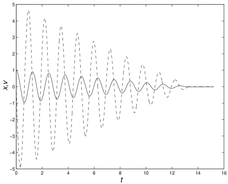
FIG. 4.: The position and the velocity as functions of time $t$, for the choice of parameters $\mu_{s}=0.15$ and $\mu_{k}=0.06$. Solid line: $x(t)$. Dashed line: $v\equiv\dot{x}(t)$.

FIG. 5.: The picewise-conserved constant of motion and the total mechanical energy as functions of time $t$, for the choice of parameters $\mu_{s}=0.15$ and $\mu_{k}=0.06$. Solid line: ${\cal E}(t)$. Dashed line: $T(t)$.

FIG. 6.: The orbit of the system in phase space: the momentum $p=M\dot{x}$ vs. the position $x$, for the choice of parameters $\mu_{s}=0.15$ and $\mu_{k}=0.06$.

Of course, the motion will not continue forever: Because of the decrease in the amplitude of the motion, eventually the static friction force at some turning point would be larger than the elastic force exerted on the block by the spring. Namely, at $t=nP_{1/2}$ we find $x(t=nP_{1/2})=(-1)^{n}(\ell-2n\mu_{k}g/\omega^{2})$, for some integer $n$, and the motion will stop for $\mu_{s}g\geq\omega^{2}(\ell-2n\mu_{k}g/\omega^{2})$, or after an integral number of phases which is equal to the least integer $n$ which satisfies

$$n\geq\frac{1}{2}\left(\frac{\omega^{2}\ell}{\mu_{k}g}-\frac{\mu_{s}}{\mu_{k}}\right).$$ (25)

We note that for the special case where $\omega^{2}\ell^{2}/(\mu_{k}g)$ is integral the block may stop at $x=0$. This happens, however, only for special values of the parameters of the systems, and in general the system will rest at $x\neq 0$.

Then, the block would remain at rest, and ${\cal E}$ would be a constant of motion from then on. Namely, because of the dissipative nature of the problem, eventually the piecewise-conserved constant of motion becomes a true constant of motion, but this happens only when the dynamics of the system becomes trivial. (In our case, when the system is in a constant state of rest.) This feature of the dissipative system is in contrast with other piecewise-conserved constants of motion, which arise from non-dissipative systems, such as the truncated Kepler problem or the three-dimensional isotropic harmonic oscillator, where the piecewise-conserved constant vector remains piecewise conserved for all times.

REFERENCES

- [1] Goldstein H 1980 Classical Mechanics 2nd edn (Reading: Addison-Wesley)
- [2] Fradkin D M 1967 Existence of the Dynamic Symmetries and for All Classical Central Potential Problems Prog. Theor. Phys. 37 798-812
- [3] Buch L H and Denman H H 1975 Conserved and piecewise-conserved Runge vectors for the isotropic harmonic oscillator Am. J. Phys. 43 1046-1048
- [4] Heintz W H 1974 Determination of the Runge-Lenz vector Am. J. Phys. 42 1078-1082
- [5] Peres A 1979 A classical constant of motion with discontinuities J. Phys. A 12 1711-1713
- [6] Serebrennikov V B and Shabad A E 1971 Method of calculation of the spectrum of a centrally symmetric Hamiltonian on the basis of approximate and symmetry Teor. Mat. Fiz. 8 23-26 [English translation: Theor. Math. Phys. 8 644-653]
- [7] Lapidus I R 1970 Motion of a Harmonic Oscillator with Sliding Friction Am. J. Phys. 38 1360-1361
- [8] Hudson R C and Finfgeld C R 1971 Laplace Transform Solution for the Oscillator Damped by Dry Friction Am. J. Phys. 39 568-570
- [9] Barratt C and Strobel G L 1981 Sliding friction and the harmonic oscillator Am. J. Phys. 49 500-501
- [10] Zonetti L F C et al. 1999 A demonstration of dry and viscous damping of an oscillating pendulum Eur. J. Phys. 20 85-88
- [11] Landau L D and Lifshitz E M 1976 Mechanics 3rd edn (Oxford: Pergamon)