High precision atom interferometry in a microgravity environment

Abstract

We propose a set of experiments in which Ramsey-fringe techniques are tailored to probe transitions originating and terminating on the same ground state level. When pulses of resonant radiation, separated by a time delay $T,$ interact with atoms, it is possible to produce Ramsey fringes having widths of order $1/T$. If each pulse contains two counterpropagating travelling wave modes, the atomic wave function is split into two or more components having different center-of-mass momenta. Matter-wave interference of these components leads to atomic gratings, which have been observed in both spatially separated fields and time separated fields. Time-dependent signals can be transformed into frequency dependent signals, leading to ground state Ramsey fringes (GSRF). The signals can be used to probe many problems of fundamental importance:

- If a gravitational field is present, the atomic gratings acquire an additional phase shift. For ground based experiments the shift can be used to obtain a precise measurement of the gravitational acceleration $g$. For experiments in a microgravity environment, GSRF can be used to measure residual gravitational fields that can be as small as $6\,10^{-9}g.$

- When atoms move in a rotating frame, the atomic grating acquires an additional phase caused by Coriolis acceleration, which also leads to a shift of the GSRF line-center. We propose to use GSRF as the basis for a new type of gyroscope. Very preliminary estimates show that in a microgravity environment one can measure a rotation rate with an accuracy of $6\,10^{-3}{{}^{\circ}}/h$, which is 10 times better than that achieved using a fiber optic gyroscope.

- Since atomic scattering from the pulses is accompanied by a momentum change, i. e. by recoil, a modulation of the grating dependence with time delay $T$ occurs. This modulation, whose frequency is equal to the atomic recoil frequency, leads to recoil splitting of the GSRF signal. The recoil splitting can be resolved with relative accuracy $10^{-6}$ and used for recoil frequency measurements, important for a precise determination of Planck’s constant.

Since only transitions originating and terminating on the same ground state are involved, frequency measurements can be carried out using lasers phase-locked by quartz oscillators having relatively low frequency. Our technique may allow one to increase the precision by a factor of 100 (the rf- to quartz oscillator frequencies ratio) over previous experiments based on Raman-Ramsey fringes or reduce on the same factor requirements for frequency stabilization.

I Introduction

Recent progress in cooling and trapping of neutral atoms allows one to observe extremely slow processes involving atoms in their ground states. These processes can serve as the basis for a new generation of atomic clocks whose operation is based entirely or partially on matter-wave interferometry.

For atoms having a velocity spread of order $1\,$cm/s that are confined to an interaction volume of $1\,$cm${}^{3},$ one can observe the evolution of various ground-state coherences for times $T_{e}$ of order $1\,$s. The line widths associated with these coherences can be as small as $0.15\,$Hz, allowing for frequency measurements having an accuracy of order $0.01-1\,$mHz. Very often, the earth’s gravitational field is the limiting factor that determines the accuracy one can achieve in these measurements. The most important effect of the Earth’s gravitational field is to introduce a Doppler frequency shift in matter-radiation field interactions. These shifts can be significant in high precision measurements of atomic recoil or rotational sensing. For experiments carried out on the time scale of $1\,s$, atoms are accelerated in the Earth’s field to a velocity of $10^{3}$ cm/s, which leads to a Doppler shift on the order of $10$ MHz. This large Doppler shift can often obscure the small recoil or rotational shifts one is attempting to measure in high precision experiments. As a result, it would be useful and important to use a microgravity environment to carry out high precision measurements of fundamental constants and inertial effects, where such measurements could be carried out with unprecedented precision. In addition to the advantages gained by elimination of the gravitational Doppler shift, one also finds that the atom-field interaction time can be increased since atoms do not fall out of the atom-radiation field interaction region as a result of gravitational acceleration.

In this article we discuss a new technique for precision measurements based entirely on matter wave interference, where one produces coherences between different atomic center-of-mass states within the same internal state. For the current state of atom interferometry, see [2]. The exclusion of any internal transitions allows one either to increase the measurement accuracy, or, for a fixed accuracy, to reduce the requirements for frequency stabilization.

The article is arranged as follows. In the next section we compare briefly different techniques to estimate the advantages of the matter wave interference method. In sections III and IV we present our previous results for gravitational acceleration and recoil frequency measurements. The ground state Ramsey fringe technique (GSRF) is discussed in Sec. V. In Sec. VI we estimate the residual gravity measurement in the microgravity environment. Sec. VII is devoted to an atom gyroscope in a microgravity environment and in a ground-based experiment. One possibility for increasing experimental precision by producing higher order atom gratings is discussed in Sec. VIII. An observation of these gratings using a 3-pulse echo technique is presented in Sec. IX. The results are summarized in Sec. X.

II Comparison of the different techniques

Even in a microgravity environment the time of evolution $T_{e}$ is still restricted by the instability of the laser frequency that produces this coherence. If the coherence oscillates at a frequency $\omega_{e}$ with stability $\alpha,$ then evidently the limitation on $T_{e}$ is given by

$$T_{e}\lesssim\left(\alpha\omega_{e}\right)^{-1}.$$ (1)

Typically, the Ramsey technique [3] is used for precise measurements, where one applies two or more resonant pulses separated by a time delay $T\sim T_{e}.$ If a resonant optical field having frequency $\Omega$ and wave vector ${\bf k}$ (see fig. 1a) excites an atom from the initial state $\left|i,{\bf p}\right\rangle$ to the final state $\left|f,{\bf p+}\hbar{\bf k}\right\rangle,$ where ${\bf p}$ and ${\bf p+}\hbar{\bf k}$ are the initial and final atomic center-of-mass momenta, and $i$ and $f$ label internal degrees of freedom, the atom coherence evolves in free space at a frequency

$$\omega_{atom}=\frac{\varepsilon_{f,{\bf p+}\hbar{\bf k}}-\varepsilon_{i,{\bf p}}}{\hbar}=\omega_{fi}+{\bf k}\cdot{\bf v+}\omega_{k},$$ (2)

where the state energy $\varepsilon_{f,{\bf p}}$ consists of the internal energy $\varepsilon_{f}$ and kinetic energy $p^{2}/2m,$ $m$ is an atom mass, $\omega_{fi}$ is a transition frequency, ${\bf v}={\bf p/}m$ is an atomic velocity, $\omega_{k}=\hbar k^{2}/2m$ is a recoil frequency. For a time $T$ between successive pulses, the atom coherence and field acquire different phases, $\omega_{atom}T$ and $\Omega T$, respectively. For the single-photon Ramsey fringe technique sensitive to this phase difference, this leads to an atom- field dephasing $\phi$ that consists of three parts, [4]

$$\phi = \phi_{R}-\phi_{D}-\phi_{q},$$ (4)

$$\phi_{R} = \Delta T,$$ (5)

$$\phi_{D} = {\bf k}\cdot{\bf v}T,$$ (6)

$$\phi_{q} = \omega_{k}T,$$ (7)

where $\Delta=\Omega-\omega_{fi}$ is the atom-field detuning. These three parts play qualitatively different roles.

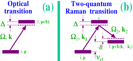
FIG. 1.: Comparison between one photon (a) and Raman (b) techniques.

The Ramsey phase $\phi_{R}$ leads to Ramsey fringes which one uses for frequency stabilization to create precise atomic clocks. For a given measure of the frequency stability $\alpha,$ the limit for the time evolution of the coherence is given by

$$T_{e}\lesssim T_{opt}\sim\left(\alpha\Omega\right)^{-1}$$ (8)

In the rf domain the Doppler phase, $\phi_{D}\ll 1$, can be neglected. On the other hand, in the optical domain, $\phi_{D}>1$ and, on averaging over the velocity distribution, the Ramsey fringe signal is destroyed[7]. The washing out of the signal is analogous to that which occurs in free induction decay (FID). The signal can be restored by the use of echo techniques involving multiple pulses of standing-wave fields[8] and/or counterpropagating optical fields. (If one uses copropagating traveling waves, the Ramsey phase and the Doppler phase both go to zero at the time the echo signal is generated.) Optical Ramsey fringes using three spatially separated standing waves were observed first in Ne on the transition at $\lambda=0.5882$ $\mu$ [9].

In contrast to the washing out of the macroscopic atom coherence, the Doppler phase can play a positive role in the optical domain. When the atom velocity changes owing to external forces, a total cancellation of the Doppler phase does not occur. If the atom acceleration is independent of the projection of the velocity along the wave propagation direction, the residual Doppler dephasing does not wash out the Ramsey fringes, but it can lead to a shift or deformation of the Ramsey fringe line shape. Therefore, optical Ramsey fringes can serve as a sensor of atomic acceleration[10]. They were used first for this purpose in Ca on the transition at $\lambda=0.6527$ $\mu m$ [11] to measure a rotation frequency.

Owing to multiphoton processes in an atom’s interaction with a standing wave field, quantum dephasing (7) is responsible for the recoil splitting of optical Ramsey fringes[12] into components centered at

$$\Delta\sim\pm\omega_{k},$$ (9)

first observed also on the transition in Ca [13].

It has proven advantageous to substitute a two-photon Raman transition between different atomic ground state hyperfine sublevels [14] for the one-photon optical transitions (see fig. 1b). Consider the interaction of an atom with two optical waves having frequencies $\Omega_{1}$ and $\Omega_{2}$, both nearly resonant with the coupled atomic transitions $i\rightarrow c$ and $c\rightarrow f,$ respectively, where $i$ and $f$ are the initial and final hyperfine sublevels of the atomic ground state. When the detunings, $\Delta_{1}$ and $\Delta_{2}$, are larger than the inverse pulse duration, it is possible to drive a two-quantum transition between states $i$ and $f$ which is resonant when

$$\delta=\Omega_{2}-\Omega_{1}+\nu_{rf}$$ (10)

is equal to 0. When an atom interacts with separated pulses, where each pulse consists of a pair of fields having frequencies $\Omega_{1}$ and $\Omega_{2}$, the Ramsey phase becomes

$$\phi_{R}=\delta T.$$ (11)

If ${\bf k}_{1}$ and ${\bf k}_{2}$ are wave vectors of the fields, absorption from mode $\left(\Omega_{1},\,{\bf k}_{2}\right)$ and stimulated emission into mode $\left(\Omega_{2},\,{\bf k}_{2}\right),$ leads to a momentum change for the atoms given by ${\bf p}\rightarrow{\bf p}+\hbar{\bf q,}$ where

$${\bf q=k}_{1}{\bf-k}_{2}.$$ (12)

The atomic coherence $i\rightarrow f$ oscillates now at the frequency

$$\omega_{atom}=\frac{\varepsilon_{f,{\bf p+}\hbar{\bf q}}-\varepsilon_{i,{\bf p}}}{\hbar}.$$ (13)

From a comparison with Eq. (2), one concludes that for a qualitative consideration of Ramsey fringes on two-quantum transitions, one can simply substitute

$${\bf k\rightarrow q=k_{1}-k_{2}}.$$ (14)

in Eqs. (6, 7) to obtain Doppler and quantum dephasings,

$$\phi_{D} = {\bf q}\cdot{\bf v}T,$$ (16)

$$\phi_{q} = \omega_{q}T,$$ (17)

respectively.

The effective wave vector $q$ changes from $0$ for copropagating waves to $2k$ for counterpropagating waves. Consequently, dephasing can be equal to or greater than the dephasing for optical Ramsey fringes. Shifts of the line center caused by quantum, inertial, or gravitational effects are also of the same order of magnitude. However, the shifts are now measured relative to the rf transition frequency, $\nu_{rf}$. Even though the line width of each laser oscillating at the frequencies $\Omega_{1}$ and $\Omega_{2}$ could be of order of 1 MHz, modern stabilization techniques allow [15] one to control the frequency difference, $\Omega_{1}-\Omega_{2}$, with a precision $\alpha\nu_{rf},$ and, therefore, the evolution time of the coherence is restricted by

$$T_{e}\lesssim T_{Raman}\sim\left(\alpha\nu_{rf}\right)^{-1}$$ (18)

Compared with the evolution time (8) allowed by the optical transition, the time (18) can be up to a factor

$$A\sim\frac{T_{Raman}}{T_{opt}}\sim\frac{\Omega}{\nu_{rf}}\sim 10^{4}\ to\text{ }10^{5}.$$ (19)

larger, which allows one to increase tremendously the accuracy of precision measurements.

The Raman-Ramsey technique was used [16] to measure the recoil frequency $\omega_{q}$ in Cs (transition $\nu_{rf}\approx 9.2\,$GHz) with an accuracy $1.1\times 10^{-7}$. This measurement is important for a precise determination of the fine structure constant [16]. A sensitivity to gravitational acceleration at the level $3\times 10^{-8}g$ has been observed [17] using the Raman-Ramsey resonance in sodium atoms (transition $\nu_{rf}\approx 1.7\,$GHz). An atom gyroscope operating on the transition in Cs has been created[18] as well, which can have a long term stability of $10^{-5}$ ${{}^{\circ}}/h$ for rotation measurements [19].

In the progression from ”one-photon optical Ramsey fringes” to ”two-quantum Raman-Ramsey fringes”, we propose the next natural step for experiments with fields separated in time or space. Only optical transitions $i\rightarrow c$ and $c\rightarrow f$ are responsible for the Doppler and recoil effects, while the transition $i\rightarrow f$ is not relevant to these effects. On the other hand the $i\rightarrow f$ transition frequency still restricts the time of evolution. It cannot be decreased out of the microwave range since atom hyperfine transition frequencies belong to this region. The restriction can only be relaxed [20] if both the final and initial internal states coincide (see fig. 2). In this case only a transition between different center-of-mass states, ${\bf p}\$and ${\bf p}+n\hbar{\bf q}$, occurs. According to a classification of atom interferometers,[21] this scheme belongs the class, matter wave atom interferometers (MWAI).

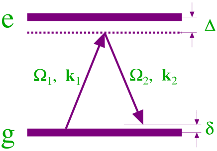
FIG. 2.: Matter wave interference scheme.

There is no inherent reason why MWAI would produce worse measurement errors than the Raman-Ramsey technique, but owing to the absence of any internal transitions, the MWAI has the potential to provide more precise measurements. Indeed, the interference between initial and final states

$$\Psi_{in}\propto\exp\left(i{\bf p}\cdot{\bf r/}\hbar\right)\text{ and }\Psi_{out}\propto\exp\left[i\left({\bf p+}\hbar{\bf q}\right)\cdot{\bf r/}\hbar\right]$$ (20)

leads to a grating in the atomic ground state population

$$\rho_{gg}\left({\bf r}\right)\propto\cos\left({\bf q}\cdot{\bf r}\right).$$ (21)

We propose to use this grating as a sensor of the gravity, inertial, and quantum effects, instead of the coherence $i\rightarrow f$ in the Raman-Ramsey scheme. The quantum dephasing (17) affects only the population grating amplitude . The velocity-dependent part of the Doppler phase (16) is canceled at an echo time, and by avoiding internal transitions, we exclude any restrictions on increasing the grating evolution time $T_{e}$ that might arise from the physics of the atom-field interaction.

The restriction on $T_{e}$ is rather technical. A small detuning $\delta$ (of order of several mHz) definitely resides within the noise bandwidth of the fields $\left(\Omega_{1},{\bf k}_{1}\right)$ and $\left(\Omega_{2},{\bf k}_{2}\right)$. Therefore, these fields cannot be detuned by $\delta$ directly. To detune them, one can use highly stabilized quartz oscillators 1 and 2 operating on the frequencies $f$ and $f+\delta$, respectively, where $f$ is a typical quartz oscillator frequency. The only requirement in choosing $f$ is that it be larger than the lasers’ noise bandwidth. A sequence of detunings of lasers 1, 2 and 3, as shown in fig. 3, controlled by quartz oscillators 1 and 2, solves the problem.

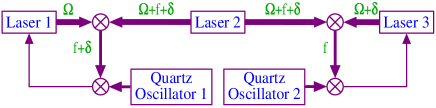
FIG. 3.: To detune lasers 1 and 3 by a small detuning $\delta$ one can use an intermediate laser 2, detune it from laser 1 by the frequency $f+\delta$ and control this detuning by a quartz oscillator 1. After that one detunes laser 3 from laser 2 by a frequency -$f$ controlled by the quartz oscillator 2.

For this scheme the evolution time of the grating is restricted by the quartz oscillator frequency instability $\alpha f,$

$$T_{e}\lesssim T_{MWAI}\sim\left(\alpha f\right)^{-1}.$$ (22)

Comparing this result with the inequality (18), one finds that using the same initial and final states allows one to increase the measurement time by a factor

$$A\sim\frac{T_{MWAI}}{T_{Raman}}\sim\frac{\nu_{rf}}{f}\sim 10^{2}-10^{3},$$ (23)

where we assume for $f$ a typical value $\left(10-100\,MHz\right).$ Even if for other reasons, such as a wave front curvature or magnetic field gradient, a further increase of the evolution time becomes impossible, our scheme still has an advantage. For a given $T_{e}$ using MWAI, one has to have the frequency stability

$$\alpha\lesssim fT_{e},$$ (24)

while for the Raman-Ramsey technique one has to stabilize frequency to $\alpha\lesssim\nu_{rf}T_{e},$ which is a factor (23) more severe.

III Earth gravity measurement

In the remaining parts of the article, we describe our current results and estimate the measurement accuracy one can achieve in ground based experiments and in microgravity measurements. We observed MWAI using a time-domain interferometer[22]. Two off-resonant standing wave pulses separated by a time $T$ are applied to a sample of cold ($150\ \mu{\rm K}$) ⁸⁵Rb atoms. The first laser pulse imposes a spatial phase modulation on the initial atomic state, which, due to the dispersion of de Broglie waves in free space, evolves into an amplitude modulation (representing an atomic population grating). Owing to the Doppler dephasing, this grating decays in a time of $1\mu s.$ Applying a second pulse, one restores gratings at the echo points,

$$T_{e}=(N+1)T,$$ (25)

where $N$ is an integer.

In our experiments, ⁸⁵Rb atoms are first cooled from a room-temperature vapor in a magneto-optical trap (MOT). Approximately 12 msec after the trapping laser beams and magnetic field are turned off (in order to allow eddy currents to die out), the two off-resonant (between 30 and 100 MHz detuning) standing wave pulses ($\sim 100\$ns duration) are applied. The standing wave pulses are composed of two traveling waves (in directions ${\bf{k}}_{1}$ and ${\bf{k}}_{2}$), switched on and off independently by a pair of acousto-optic modulators (AOM). The AOMs are driven by a common radio frequency (rf) oscillator operating at 220 MHz (see Fig. 4). The atomic grating is probed by switching on only the traveling wave along ${\bf{k}}_{2}$ and measuring the (complex) amplitude of the wave scattered into the direction ${\bf{k}}_{1}$.

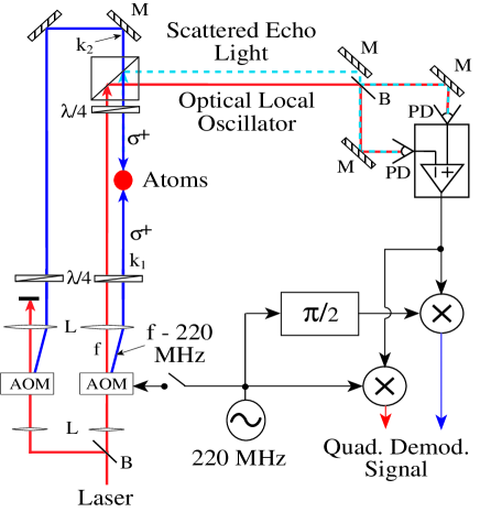
FIG. 4.: Schematic diagram of the experimental setup. M = mirror, B = beam splitter, PD = Photodiode, AOM = Acousto-optic modulator, $\lambda/4=$ Quarter-wave plate, L = Lens, PBS = Polarizing Beam Splitter, and $\bigotimes$ = Mixer.

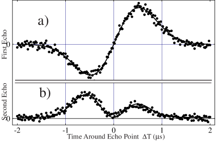
FIG. 5.: Representative examples of the scattered signal as a function of $\Delta t=t$ - $T_{e}$ for (a) $T_{e}=2T$, and (b) $T_{e}=3T,$ $t$ is the total elapsed time from the first pulse. The data in part (a) were taken using $\sigma^{+}$ polarized standing wave pulses, $T=799\ \mu{\rm s}$. In (b), linearly polarized pulses were used, $T=19\ \mu{\rm s}$.

The scattered wave is detected by beating it with an optical local-oscillator in a balanced heterodyne arrangement. The local oscillator is derived from the light passing undiffracted through the AOM used to switch the ${\bf{k}}_{1}$ beam. During the experiment, the echo beat signal is further mixed down by a 220 MHz reference from the rf oscillator using a quadrature demodulator. The two outputs of this demodulator represent the real and imaginary parts of the scattered light field, where the real part is in phase with the ${\bf{k}}_{1}$ field (which is not on during detection), and the imaginary part is $\pi/2$ out of phase with ${\bf{k}}_{1}$.

Typical time-dependences of the scattered signal amplitudes in the vicinity of the echo points $T_{e}=2T$ $\left(N=1\right)$ and $T_{e}=3T$ $\left(N=2\right)$ are shown in Fig. 5.

Since our detection scheme is sensitive to the phase of the scattered signal, it is possible to measure the influence of the gravitational acceleration ${\bf g}$. The acceleration changes an atom trajectory and the Doppler phase (16). The time dependence of the atom grating Doppler phase is shown in the Fig. 6.

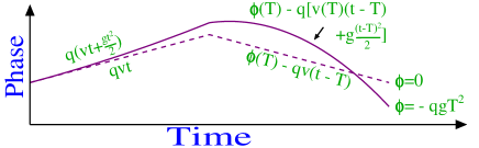
FIG. 6.: Echo phase diagram for free space (dashed line) and in the presence of gravity (solid line).

We show here the process responsible for the echo at $T_{e}=2T.$ The first pulse produces an atom grating evolving as $\exp\left[-i{\bf q}\cdot r\left(0\right)\right],$ where ${\bf r}\left(0\right)$ is the atom position at $t=0.$ A nonlinear 4-quantum interaction with second pulse results in the atom grating evolving as $\exp\left[-i{\bf q}\cdot r\left(0\right)+2i{\bf q}\cdot r\left(T\right)\right].$ For a given space time point $\left({\bf r},t\right)$ this dependence can be represented as

$$\rho_{gg}\left({\bf r}\right)\propto\exp\left(i{\bf q}\cdot{\bf r+}i\phi_{D}\right),$$ (26)

where the Doppler phase $\phi_{D}$ consists of two parts

$$\phi_{D}\left(t\right) = \phi_{1}+\phi_{2},$$ (28)

$$\phi_{1} = {\bf q}\cdot\delta{\bf r}_{1},$$ (29)

$$\phi_{2} = -{\bf q}\cdot\delta{\bf r}_{2},$$ (30)

$\delta{\bf r}_{1}$ and $\delta{\bf r}_{2}$ are the atomic displacements between $0$ and $T$ and between $T$ and $t.$ Without gravity $\delta{\bf r}_{1}={\bf v}T,\,\,\delta{\bf r}_{2}={\bf v}(t-T)$ and the phases $\phi_{1,2}$ cancel one another at the echo point. In a gravitational field,

$$\delta{\bf r}_{1} = {\bf v}T+{\bf g}T^{2}/2$$ (32)

$$\delta{\bf r}_{2} = {\bf v}\left(T\right)\left(t-T\right)+{\bf g}\left(t-T\right)^{2}/{2,}$$ (33)

where ${\bf v}$ is the initial velocity, ${\bf v}\left(T\right)={\bf v}+{\bf g}T$. Cancellation of the Doppler phase dependence on ${\bf v}$ still occurs at $t=2T,$ but a residual gravity dependent part $\phi_{{\bf g}}$ arises which is equal to

$$\phi_{{\bf g}}\equiv\phi_{D}\left(2T\right)={\bf q}\cdot{\bf g}T^{2}.$$ (34)

We observe this dependence. Fig. 7 shows our results for the first echo ($T_{e}=2T$) in the case where ${\bf{k}}_{1}=-{\bf{k}}_{2}$ and are aligned to within 1 mrad of vertical, so the expected phase dependence on the pulse spacing is $\phi_{D}\left(2T\right)=2kg\,T^{2}$. Fig. 7(a) shows the phase as a function of pulse spacing (points) together with a solid curve corresponding to the best fit, which was obtained for $g=9.798$ m/s². Fig. 7(b) shows the difference between this best fit and the data.

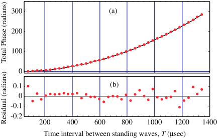
FIG. 7.: (a) Phase of the scattered signal as a function of the pulse spacing $T$. Points are the data and solid curve is the best fit. (b) Phase difference between data and best fit as a function of $T$.

IV Recoil frequency measurement.

The influence of atom acceleration arises whether or not the particles’ motion needs to be quantized. In contrast, effects related to recoil are necessarily linked with quantization of the atomic center-of-mass motion [23]. The quantum part of dephasing (17) arises as a result of quantization. This part leads to the periodic dependence of the echo amplitude on the time delay between pulses. The period is given by

$$\Delta T=\pi/\omega_{q}.$$ (35)

Observation of the periodical dependence allows one to measure precisely the recoil frequency

$$\omega_{q}=\hbar q^{2}/2m,$$ (36)

which is important for precise determination of the fundamental constants [16]. The best accuracy of this measurement can be achieved in a microgravity environment.

We observed [22] oscillation of the atom grating amplitudes. Examples of the oscillating dependences are shown in Fig. 8.

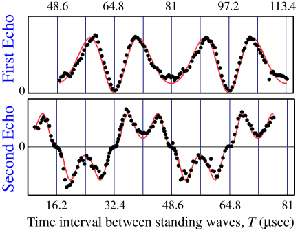
FIG. 8.: Amplitude of the scattered signal (determined from the fits shown in Fig. 5) as a function of the pulse spacing $T$ for (a) $T_{e}=2T$ and (b) $T_{e}=3T$. The dots are the data and the solid line is the theoretical fit[22].

The precision $\Delta\omega_{q}$ with which one can determine the recoil frequency is given approximately by $\Delta\omega_{q}/\omega_{q}=\Delta T/T_{{\rm max}}$, where $\Delta T$ is the uncertainty in the time of the zeroes of the signal and $T_{{\rm max}}$ is the maximum value of $T$ that yields a significant signal. For our data we estimate $\Delta\omega_{q}/\omega_{q}=(100$ ns$)/(1$ ms$)=10^{-4}$. We calculated the period by measuring the time between well-displaced zeroes of the signal and dividing by the number of intervening periods. This yielded a period of $32.388\ \mu s$ [compare this with the result of $32.386\ \mu s$ calculated from Eq. (35) for transition $\lambda=0.78\mu$ in ${}^{\text{85}}$Rb].

V Ground state Ramsey fringes

The experiments described above have been carried out in the time domain. One can expect that the accuracy of measurement will be higher in the frequency domain. For this purpose we propose the ground state Ramsey fringes (GSRF) technique[20]. If traveling wave modes ${\bf k}_{1}$ and ${\bf k}_{2}$ are slightly detuned from each other by the detuning $\delta$, as shown in Fig. 2, the atom coherence (ground state population grating) acquires the Ramsey phase

$$\phi_{R}\sim\delta T.$$ (37)

For a given time delay between pulses, one can monitor the signal from a back-scattered field as a function of $\delta.$ The presence of atomic acceleration or recoil affects the positions of the GSRF maxima. One obtains another type of the acceleration or recoil effect sensor which, in contrast to the Raman-Ramsey fringes, has the potential to increase the time of the measurement beyond the limit imposed by the large frequency of the involved internal transitions.

The scheme of the GSRF is shown in fig. 9. The first pulse produces a grating which acquires the Ramsey phase (37), but it decays fast owing to the large Doppler phase (16). For the second pulse, we propose to reverse the directions of the travelling waves with respect to the first pulse. If the second pulse were identical to the first, then the Ramsey and Doppler phases would be mutually constrained: they enter into the grating phase only in the combination $\phi_{R}-\phi_{D}$ and, therefore, a cancellation of the Doppler phase coincides with a loss of the Ramsey phase. But, if one reverses the directions of the travelling waves, then non-linear processes become possible where the Doppler phases acquired during the time intervals, $\left[0,T\right]$ and $\left[T,2T\right]$, are canceled while the Ramsey phases acquired during these intervals add to one another.

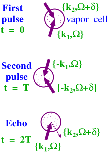
FIG. 9.: Field geometry to observe GSRF

Finally, the third, readout pulse, consisting of only one traveling mode $\left\{{\bf k}_{1},\Omega\right\},$ scatters off the atom grating into the field mode $\left\{{\bf k}_{2},\Omega+\delta\right\}$ radiated by the vapor. This signal contains the Ramsey fringes, i. e. the oscillating dependence on the Ramsey phase (37).

VI Residual gravity measurement in a microgravity environment

The extreme sensitivity of the GSRF signal to small perturbations of the atomic center-of-mass motion makes it ideal for acceleration measurements in a microgravity environment. A program for carrying out such measurements [the Space Acceleration Measurement System (SAMS)] is part of the NASA program [28]. The sensors of residual gravity are necessary to control the environmental quality. We propose to investigate the potential for GSRF measurements of residual gravity in a microgravity environment.

For further estimates of the measurement accuracy, we need a minimum measurable value of the GSRF shift $\delta.$ There is no reason for this shift to be worse than that achieved by the Raman-Ramsey technique, but, as we have explained above, for GSRF this shift can be smaller. The ultimate limit for GSRF shift will be established by experiments, either ground based or gravity free. In this article we take the lower boundary of the shift equal to

$$\delta_{\min}=2\pi\,15\,mHz.$$ (38)

One can get this value as a product of the relative accuracy $\left(1.1\,10^{-7}\right)$ of the recoil frequency measurement using the Raman-Ramsey technique [15] and $\omega_{q}$ $\left(2\pi\,130\,kHz\right).$ The halfwidth of the Raman-Ramsey fringes in the experiment of Ref.[15] was

$$\Gamma_{R}\approx 2\pi\,8\,Hz.$$ (39)

Let us estimate the minimum residual acceleration ${\bf g}_{r\min}$ which can be measured by GSRF in a cold ⁸⁵Rb vapor or beam. If GSRF in time separated fields are used, the gravitational phase shift $\phi_{g_{r}}$ in the vicinity of the $t=2T$ echo point is obtained by replacing ${\bf g\rightarrow g}_{r}$ in Eq. (34), $\phi_{g_{r}}={\bf q\cdot g}_{r}T^{2}.$ When the phase shift is small, it results in a shift of the GSRF by an amount $\delta_{g_{r}}\sim\phi_{g_{r}}/T={\bf q\cdot g}_{r}T.$ Since we assume that a frequency measurement with accuracy (38) is possible, for ${\bf q\parallel g}_{r}$ and $T=100\,ms$ one gets for a lower limit of the residual gravity measurement

$$g_{r\min}\approx 6\,10^{-9}g.$$ (40)

To measure such a small residual gravity, one has to exclude corrections arising from rotations. Rotation with frequency $\Omega_{r}$ leads to a Coriolis acceleration of order of $2\left\langle u\right\rangle\Omega_{r},$ where $\left\langle u\right\rangle$ is the mean atomic velocity. In an atomic beam launched with velocity $u=17\,cm/s,$ the requirement that the Coriolis acceleration produce a shift less than the minimum residual gravitational shift given by Eq. (40) can be stated as

$$\Omega_{r}<3\,10^{-3}\Omega_{earth}.$$ (41)

The situation improves if one uses a cold atomic vapor, such as that used in our experiment[22] and in experiments on optical transitions in Mg[29]. The corrections from rotation would vanish identically if the mean velocity of the vapor were identically equal to zero. If there is some asymmetry in the distribution that gives rise to a mean velocity $\left\langle u\right\rangle=\alpha\Delta u,$ where $\Delta u$ is the width of the velocity distribution, then it is necessary that

$$\alpha<g_{r\min}/2\Delta u\Omega_{r}.$$ (42)

for rotational effects to be negligible. Even if the space station rotates with the earth’s rotation rate, for the transition in ⁸⁵Rb and $\Delta u=17\,cm/s,$ one finds that $\alpha<3\,10^{-3}$ is needed. This less severe restriction shows that it is better to use cold vapors than beams for precise measurements of residual gravity.

VII Atom gyroscope

In this section we estimate the precision of an atomic gyroscope based on GSRF. Estimates have to be performed separately for the microgravity environment and ground-based experiment.

A Atom gyroscope in a microgravity environment.

We propose to use GSRF as a sensor of a system’s rotation. When Ramsey fringes are observed in a frame rotating with angular frequency ${\bf\Omega}_{r}$, the atoms undergo a Coriolis acceleration equal to

$${\bf a=}2{\bf v\times\Omega}_{r}.$$ (43)

Owing to this acceleration, a new type of dephasing $\phi_{r}$ arises[10]. To obtain this dephasing for a small rotation rate, one can neglect changes of the acceleration resulting from changes in the atomic velocity. In this limit, one can simply replace ${\bf g}$ by ${\bf a}$ in Eq. (34) to obtain the rotational dephasing $\phi_{r}$ given by

$$\phi_{r}=2\left({\bf q\times\Omega}_{r}\right)\cdot{\bf v}T^{2}.$$ (44)

A direct observation of this fringe shift has been reported previously using microfabricated structures to scatter atoms [24, 25]. A precision of

$$\delta\Omega_{r}=0.042\text{ }\Omega_{earth}=0.63\,{{}^{\circ}}/h,$$ (45)

where $\Omega_{earth}=15{{}^{\circ}}/h$ is the earth rotation rate, has been achieved [25]. We have already discussed rotational observations using optical Ramsey fringes [11] and Raman-Ramsey fringes[18, 19]. In the latter case the precision is

$$\delta\Omega_{r}=6\text{\thinspace}10^{-3}\Omega_{earth}=0.08\,{{}^{\circ}}/h.$$ (46)

This precision is still below that of fiber-optic-gyroscopes [26] $\left(0.047\,{{}^{\circ}}/h\right)$, but already better than that of ring-laser gyroscopes[27] $\left(0.18\,{{}^{\circ}}/h\right)$.

One can use the Ramsey resonance shift as a rotation sensor[10, 11]. In contrast to measurements of photon recoil effects or gravitational acceleration which can be measured using either temporally or spatially separated pulses, gyroscopic measurements involving frequency measurements should be carried out using spatially separated fields[10]. A scheme for accomplishing this using GSRF is shown in Fig. 10.

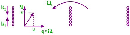
FIG. 10.: Gyroscope based on ground state Ramsey fringes.

If the rotation frequency is perpendicular to ${\bf q}$, the rotation phase (44) is equal to $\phi_{r}=2q\Omega_{r}sign\left(u\right)L^{2}/u$, where $L=uT$ is the spatial separation of the fields. The Ramsey phase $\phi_{R}=2\delta T=2\delta L/u$ has the same dependence on longitudinal velocity $u$ as $\phi_{r}$. The total phase is

$$\phi=\phi_{R}+\phi_{r}=2\left(\delta+qL\Omega_{r}\right)/u.$$ (47)

The Ramsey fringes are centered at the point where $\phi=0$. As a result of the rotation, the central fringe is shifted by

$$\delta=-sign\left(u\right)qL\Omega_{r}.$$ (48)

The highest gyroscope accuracy can be reached in a microgravity environment. If an effusive beam of atoms with thermal velocity $u$ crosses three interaction zones, each separated from one another by distance $L,$ than the Ramsey fringes halfwidth is given by [6]

$$\Gamma_{R}\approx 0.6u/L.$$ (49)

The distance between fields $L$ can be chosen arbitrarily. A large distance allows for a more precise measurement of the rotation frequency. We set $L=20\,$cm in arriving at our estimates. For the fringe halfwidth (39) and $u\approx 20\,m/s$ on a transition in ${}^{\text{85}}$Rb $\left(\lambda=0.78\mu,q=1.6\,10^{5}\,cm^{-1}\right)$ with the shift given by Eq. (38), the minimum measurable rotation rate is equal to

$$\Omega_{r\min}\sim 4\,10^{-4}\Omega_{earth}\approx 6\,10^{-3}{{\,\,}^{\circ}}/h.$$ (50)

B GSRF gyroscope in ground based measurements

In principle, the same accuracy (50) can be achieved in ground based experiments, but for this purpose the wave vectors ${\bf k}_{i}$ have to be aligned in the horizontal plane to exclude gravitational influence. Let us estimate the requirements for this alignment. The typical time of flight of atoms between separated fields is $T\sim L/u\sim 1.5$/$\Gamma_{R}\approx 30\,ms.$ If $\theta$ is the order of magnitude of the small residual angle between the wave vectors and the horizontal plane, then the gravitational phase (34), $\phi_{g}\sim qg\theta T^{2},$ leads to the GSRF shift $qg\theta T$. When we require this to be smaller than the minimum measurable shift (38), one finds that for a transition in ⁸⁵Rb,

$$\theta\lesssim\frac{\lambda\delta_{\min}}{4\pi gT}\approx 2\,10^{-8}\,rad,$$ (51)

which is two orders more severe than the present state-of-the-art limit for alignment [30].

For the further elimination of gravity in ground based measurements, one can observe simultaneously two scattered signals, I and II (see Fig. 11). These signals both contain GSRF’s, whose shifts $\delta_{I,II}$ consist of gravitational and rotational parts $\delta_{I,II}^{g}$ and $\delta_{I,II}^{r}$. From Fig. 11, one concludes that signal II is produced by the fields consisting of traveling wave field modes $\left(\mp{\bf k}_{2},\Omega+\delta\right)$ and $\left(\mp{\bf k}_{1}{\bf,}\Omega\right)$ instead of modes $\left(\pm{\bf k}_{1}{\bf,}\Omega\right)$ and $\left(\pm{\bf k}_{2},\Omega+\delta\right)$ responsible for signal I (signal II is obtained from signal I by the substitutions ${\bf k}_{1}{\bf\leftrightarrow-k}_{2},$ $\Omega\leftrightarrow\Omega+\delta)$. Under this transformation the wave vector difference ${\bf q}$ given by Eq. (14) is not changed, but the detuning $\delta$ changes sign. Thus, the gravity-induced parts of the shifts have opposite sign, $sign\left(\delta_{II}^{g}\right)=-sign\left(\delta_{I}^{g}\right),$ and the sum of the shifts $\delta=\delta_{I}+\delta_{II}$ is gravity insensitive provided that the fields are imposed symmetrically with respect to the symmetry axis of the atomic spatial-velocity distribution (dashed arrow on the Fig. 11). A similar idea for eliminating the effects of gravity in rotation measurements has been considered recently[31] and realized in the Raman-Ramsey gyroscope[19].

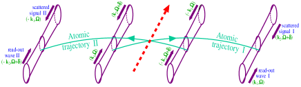
FIG. 11.: A scheme of the atomic gyroscope in the presence of the earth’s gravity field.

This severe requirement for the atomic phase space distribution to have a symmetry axis is easier to realize for atoms in a cell in thermal equilibrium than in counterpropagating atomic beams.

VIII Higher order atomic gratings.

To increase the sensitivity to an atom’s acceleration, one can use higher order atom gratings having wave numbers that are a multiple of $q.$ The nonlinear interaction of an atom with a pulse of non-copropagating fields applied to the same transition leads to higher order grating production in the atom ground state population[5, 6, 8, 9, 13, 20, 21, 22]. This is in contrast to the interaction with separated traveling waves[10, 11, 29] or counterpropagating traveling waves applied on adjacent transitions[14, 15, 16, 17, 18, 19, 31], where to get higher harmonics one needs a number of pulses[15]. (The only exception is a multiple beam atom interferometer[32].) When higher harmonics are involved in the process of grating formation, one can expect that the part of the Doppler phase (34) caused by acceleration ${\bf a}$ increases. This should allow one to increase the accuracy of the acceleration measurement. This statement is illustrated in Fig. 12, where the phases of the first and second order grating [evolving as $\cos\left({\bf q}\cdot{\bf r}\right)$ and $\cos\left(2{\bf q}\cdot{\bf r}\right)$, respectively] are compared.

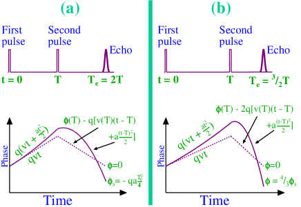
FIG. 12.: Echo phase diagrams corresponding (a) to the first-order grating localized near the echo point $T_{e}=2T$  and (b) second order grating localized near $T_{e}=\,^{3}/_{2}T$ for free space (dashed line) and in the presence of gravity (solid line).

Consider the general case. If the first strong pulse produces an atom grating evolving as $e^{in_{1}{\bf q}\cdot{\bf r}}$, this grating acquires the Doppler phase part,

$$\phi_{1}=n_{1}{\bf q}\cdot\delta{\bf r}_{1},$$ (52)

where $\delta{\bf r}_{1}$ is the atomic displacement, during the time interval $\left[0,T\right].$ Similarly, if after the second pulse the grating $e^{in{\bf q}\cdot{\bf r}}$ is produced, it acquires an additional phase during the time interval $\left[T,t\right]$,

$$\phi_{2}=n{\bf q}\cdot\delta{\bf r}_{2},$$ (53)

where $\delta{\bf r}_{2}$ is the corresponding atomic displacement. Using expressions (III) one finds that the total phase $\phi_{D}(t)$ is given by

$$\phi_{D}(t) = {\bf q}\cdot{\bf v}\left[n_{1}T+n\left(t-T\right)\right]+$$ (55)

$${}^{1}/_{2}{\bf q}\cdot{\bf a}\left[n_{1}T^{2}+n\left(t^{2}-T^{2}\right)\right].$$

The echo point is by definition, a time, $t=T_{e},$ where the velocity dependent part is canceled. One find that this cancellation occurs at all points

$$T_{e}=\frac{n^{\prime}}{n}T,$$ (56)

where $n^{\prime}=n-n_{1}$ $\left(\left|n^{\prime}\right|>\left|n\right|\right),$ integers $n^{\prime}$ and $n$ have no common factor. Since after the second pulse the grating evolves as $e^{in{\bf q}\cdot{\bf r}},$ the grating period is given by $2\pi/nq.$ One sees that the first harmonic $\left(n=1\right)$ is localized at the points $2T,$ $3T,\ldots$, the second harmonic $\left(n=2\right)$ is localized at ${}^{3}/_{2}T,$ ${}^{5}/_{2}T,\ldots$ and so on.

At the echo point the residual Doppler phase $\phi_{{\bf a}}\equiv\phi_{D}(T_{e})$ associated with acceleration ${\bf a}$ can be represented as

$$\phi_{{\bf a}}=2n(1-T/T_{e})\phi_{s},$$ (57)

where $\phi_{s}={\bf q}\cdot{\bf a}T_{e}^{2}/4$ the minimum value of $\phi_{{\bf a}}$ at the point $T_{e}=2T.$ The echo time $T_{e}$ is evidently the total time of the atomic coherence evolution. To compare acceleration-related phases, this time has to be fixed. The ratio $\phi_{{\bf a}}/\phi_{s}$ for the different grating periods and different time separation between pulses $T$ is shown in the following table

$\displaystyle\begin{array}[]{ccc}\begin{array}[]{c}Grating\\ period\end{array}&\begin{array}[]{c}Time\,\,of\\ evolution\end{array}&\frac{\phi_{a}}{\phi_{s}}\\ 2\pi/q&T_{e}/T=2&1\\ 2\pi/q&T_{e}/T=3&4/3\\ 2\pi/q&T_{e}/T=\infty&2\\ \pi/q&T_{e}/T=3/2&4/3\\ \pi/q&T_{e}/T=5/2&12/5\\ \pi/q&T_{e}/T=\infty&4\\ 2\pi/3q&T_{e}/T=4/3&3/2\\ 2\pi/3q&T_{e}/T=7/3&24/7\\ 2\pi/3q&T_{e}/T=\infty&6\end{array}$

IX Three-pulse echo technique.

In this section we describe our recent technique [33] for observing the higher order atomic gratings. Higher order gratings allow one to improve the sensitivity of inertial measurements.

In the Sec. III we described the back-scattering technique to observe atomic grating. The grating was detected by applying a traveling wave to the atomic cloud and measuring the coherent backscattering of this traveling wave. One of the properties of this detection technique is that it is sensitive only to the second harmonic of the atomic density distribution (i.e. the spatial Fourier component with period $2\pi/q$). This detection technique has the nice feature for atom interferometry experiments that the signal is not accompanied by a (possibly large) background due to the zeroth harmonic of the atomic density distribution. It has a disadvantage in that it reveals no direct information about the higher harmonics (4th, 6th, etc).

By applying a second standing wave at a time $T_{2}$ after the initial standing wave, one can rephase the 1st order grating (with periodicity $2\pi/q$) and produce high ($n$th) order gratings (with periodicity $2\pi/nq$) at various times after the this second pulse. To observe higher order gratings, we apply a third standing-wave pulse (SW3) whose purpose is to convert the higher-order grating into a 2nd-order grating that can be detected by the back-scattering technique described above.

Our experiments were carried out with a cloud of ⁸⁵Rb atoms cooled down to 105 $\mu$K in a magneto-optical trap. The cloud was illuminated by a series of three optical pulses of two $\sigma^{+}$-polarized plane waves traveling in opposite directions, ${\bf k}_{1}$ and ${\bf k}_{2}$ (see Figure 13).

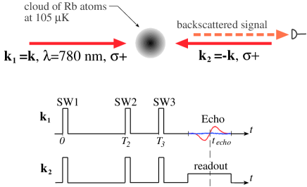
FIG. 13.: Sketch of our experiment in the MOT.

The frequency of the optical pulses was detuned above the atomic transition frequency of the ⁸⁵Rb 5S${}_{1/2}\,(F=3$) – 5P${}_{3/2}\,(F^{\prime}=4$) transition by 400 MHz. The role of spontaneous processes was therefore negligible. The first pulse (SW1) creates a spatial grating in the atomic cloud. The grating rapidly vanishes due to the Doppler dephasing. The pulse SW2 causes the reappearance of the gratings of various orders at later times (see Fig. 14).

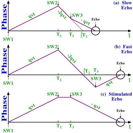
FIG. 14.: Phase diagrams of three different three-pulse echoes.

At a time in the vicinity of $(3/2)T_{2}$, where the 2nd order grating is expected to occur, we applied a third standing wave pulse. Figures 14 (a) and (b) show the effect of the third pulse on the second order grating (period $\pi/q$). Echoes occur at times when the lines cross the horizontal ($t$) axis. If the third pulse occurs  before $(3/2)T_{2}$, we call the signal the slow echo and observe the echo shown in Fig. 14(a). On the other hand, Fig. 14(b) shows the situation when the third pulse occurs after the time $(3/2)T_{2}$, which we call the fast echo. In addition, we find another echo signal that depends on all three of the standing-wave pulses, shown in Fig. 14(c). These echoes can be distinguished experimentally by measuring their time of occurrence as a function of the time of application of the excitation pulses. In particular, Figure 15 shows the time of the echoes of Fig. 14 as a function of the time of the third pulse.

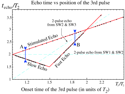
FIG. 15.: In this echo diagram, solid lines represent the echos that have been observed. The data points pertain to the three-pulse echo that we wish to study.

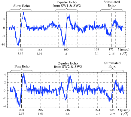
FIG. 16.: Echo signals. The two time traces correspond to A and B in Figure 15.

Around the echo time, $T_{e}$, the grating is probed by a long weak pulse with traveling wave vector ${\bf k}_{2}$. The grating backscatters in the direction ${\bf k}_{1}$. The scattered light strikes a heterodyne detector sensitive to the field amplitude and phase. The dots in figure 15 are the actual experimental data points representing times when echo signals were detected. The vertical lines marked A and B correspond to two time traces shown in figure 16. In these traces one can clearly see three different echoes, the one two-pulse and two three-pulse echoes, that fall into the selected time interval. It is interesting to notice that when the SW3 pulse is applied, the amplitude of the two-pulse echo produced by SW1 and SW2 becomes smaller. This is because a part of the phase trajectories leading to this echo is converted by SW3.

The contrast of the higher order grating can be found from the echo amplitude. We have studied the amplitude of the fast and slow echoes as a function of $T_{3}$. The experimental data and theoretical fit are shown in figure 17.

FIG. 17.: Dependence of the fast and slow echos amplitude on $T_{3}$.

Even though the theory fits the experiment well, additional study is required to be able to monitor the higher order gratings by looking at the echo signal.

To summarize, in our three-pulse experiment we successfully detected the second order atomic density grating in a MOT cloud. In addition, use of three standing wave pulses allows us not only to detect the higher order gratings, but also to convert them to yet higher orders. It is also a first step in our study of multi-pulse echoes. One intention is to measure gravitational acceleration using higher order gratings.

X Conclusion

Matter wave interference techniques can lead to significant improvements in the precise measurement of inertial, gravitational, and quantum effects.

Being insensitive to the energy of the atomic internal motion, the shape and the center of the ground state Ramsey fringes do not depend on perturbations of the internal state. Simultaneously, the accuracy of measurements is not related to any frequency of internal transitions. It allows one to increase the time of the atomic coherences’ evolution $T_{e}$ by 2-3 orders of magnitude, or reduce requirements for frequency stabilization by 2-3 orders of magnitude.

These advantages can be exploited most fully in a microgravity environment, where the experiments do not suffer the enormous gravitational dephasing of atom coherences between different center-of-mass states.

REFERENCES

- [1] B. Dubetsky, A. P. Kazantsev, V. P. Chebotayev, V. P. Yakovlev, Pis’ma Zh. Eksp. Teor. Fiz. 39, 531 [JETP Lett. 39, 649 (1985)].
- [2] Atom Interferometry, Edited by P. R. Berman, Academic Press, San Diego, New York (1997)
- [3] N. F. Ramsey, Phys. Rev. 76, 996 (1949).
- [4] Owing to relativistic corrections, dephasing caused by the second order Doppler effect also arises. This has been observed and studied independently in Refs. [5, 6].
- [5] R. L. Barger, Opt. Lett., 6, 145 (1981)
- [6] B. Dubetsky, Kvantovaya Electron. 10, 1203 (1983) [Quantum Electron 15, 1290 (1983)].
- [7] A. N. Orayevsky, IEEE Transaction on Instrument an Measurement, IM-17, No. 4, 346 (1968).
- [8] Ye. V. Baklanov, B. Dubetsky, V. P. Chebotayev, Appl. Phys. 9, 171 .
- [9] J. C. Bergquist, S. A. Lee, and J. L. Hall, Phys. Rev. Lett. 38, 159 (1977).
- [10] Ch. J. Borde, Phys. Lett. A 140,10
- [11] F. Riehle, Th. Kisters, A. Witte, J. Helmcke, Ch. J. Borde, Phys. Rev. Lett. 67, 177
- [12] B. Dubetsky, V. M. Semibalamut, In Sixth International conference on atomic physics. Abstracts, edited by E. Anderson, E. Kraulinya, R. Peterkop (Riga, USSR, 1978), p. 21.
- [13] R. L. Barger, J. C. Bergquist, T. C. English, D. J. Glaze, Appl. Phys. Lett., 34, 850 (1979).
- [14] M. Kasevich, S. Chu, Phys. Rev. Lett., 67, 181 (1991).
- [15] D. S. Weiss, B. C. Young, S. Chu, Appl. Phys. B 59, 217 (1994), Sec. 3.3.
- [16] D. S. Weiss, B. C. Young, S. Chu, Phys. Rev. Lett., 70, 2706 (1993).
- [17] M. Kasevich, S. Chu, Appl. Phys. B 54 321
- [18] T. L. Gustavson, P. Bouyer, and M. A. Kasevich, Phys. Rev. Lett. 78, 2046 (1997).
- [19] M. Kasevich. Precision atom interferometry, report on the 1999 NASA/JPL International Conference on Fundamental Physics, Washington 1999.
- [20] B. Dubetsky and P. R. Berman, Phys. Rev. A 56, R1091 (1997).
- [21] B. Dubetsky and P. R. Berman, Phys. Rev. A 59, 2269 (1999)
- [22] S. B. Cahn, A. Kumarakrishnan, U. Shim, T. Sleator, P. R. Berman, B. Dubetsky, Phys. Rev. Lett. 79, 784 (1997).
- [23] A. P. Kol’chenko, S. G. Rautian, R. I. Sokolovskii, Zh. Eksp. Teor. Fiz. 55, 1864 (1968) [JETP 28, 986 (1969)].
- [24] M. K. Oberthaler, S. Bernet, E. M. Rasel, J. Schmiedmayer, and A. Zeilinger, Phys. Rev. A 54, 3165 (1996).
- [25] A. Lenef, T. D. Hammond, E. T. Smith, M. S. Chapman, R. A. Rubenstein, and D. E. Pritchard, Phys. Rev. Lett. 78, 760 (1997).
- [26] C-X. Shi, H. Lizuka, Microwave and optical technology letters, 9, 233 (1995).
- [27] G. E. Stedham, Z. Li, C. H. Rowe, A. D. McGregor, and H. R. Birger, Phys. Rev. A, 51, 4944 (1995).
- [28] Microgravity News, 3, No 3. (1996).
- [29] U. Sterr, K. Sengstock, W. Ertmer, F. Riehle, J. Helmcke, In Atom Interferometry, Edited by P. R. Berman, Academic Press, San Diego, New York (1997), pp. 293-362 and references therein.
- [30] W. Blum, H. Kroha, P. Widmann, IEEE-Trans. Nucl. Science, 43, 1194 .
- [31] B. Young, M. Kasevich, S. Chu, In: Atom Interferometry, edited by P. R. Berman (Academic Press, Cambridge, MA, 1997), pps. 363-406, Sec. IV.C.
- [32] M. Weitz, T. Heupel, T. W. Hansch, Phys. Rev. Lett. 77, 2356 (1996); Europhys. Lett., 37, 517 (1997);Appl. Phys. B 65, 713 (1997)
- [33] A. V. Turlapov, D. V. Strekalov, A. Kumarakrishnan, S. Cahn, and T. Sleator, in ICONO’98: Quantum Optics, Interference Phenomena in Atomic Systems, and High-Precision Measurements (edited by A. V. Andreev, S. N. Bagayev, A. S. Chirkin, and V. I. Denisov), SPIE Proc. 3736, 26-37 (1999).