Ionization of a Model Atom: Exact Results and Connection with Experiment

Abstract

We prove that a model atom having one bound state will be fully ionized by a time periodic potential of arbitrary strength $r$ and frequency $\omega$. The survival probability is for small $r$ given by $e^{-\Gamma t}$ for times of order $\Gamma^{-1}$ $\sim r^{-2n}$, where $n$ is the number of “photons” required for ionization, with enhanced stability at resonances. For late times the decay is like $t^{-3}$. Results are for a 1d system with a delta function potential of strength $-g(1+\eta(t))$ but comparison with experiments on the microwave ionization of excited hydrogen atoms and with recent analytical work indicate that many features are universal.

PACS: 32.80.Rm, 03.65.Db, 32.80.Wr.

*******

Transitions between bound and free states of a system are of great importance in many areas of science [1] and “much of the practical business of quantum mechanics is calculating exponential decay rates” [2]. There are, however, still many unresolved questions when one goes beyond perturbation theory [1]–[7]. Unfortunately, approaches going beyond perturbation theory such as Floquet theory, semi-classical analysis and numerical solution of the time dependent Schrödinger equation are both complicated and also involve, when calculating transitions to the continuum, uncontrolled approximations [1]–[6]. It is only recently that some general results going beyond perturbation theory have been rigorously established for models with spatial structure [7]. We still don’t know, however, many basic facts about the ionization process, e.g. the conditions for a time dependent external field to fully dissociate a molecule or ionize an atom, much less the ionization probability as a function of time and of the form of such a field [8]. Granted that the problem is intrinsically complicated it would be very valuable to have some simple solvable models which contain the spatial structure of the bound state and the continuum and can thus serve as a guide to the essential features of the process.

In this note we describe new exact results relating to ionization of a very simple model atom by an oscillating field (potential) of arbitrary strength and frequency. While our results hold for arbitrary strength perturbations, the predictions are particularly explicit and sharp in the case where the strength of the oscillating field is small relative to the binding potential—a situation commonly encountered in practice. Going beyond perturbation theory we rigorously prove the existence of a well defined exponential decay regime which is followed, for late times when the survival probability is already very low, by a power law decay. This is true no matter how small the frequency. The times required for ionization are however very dependent on the perturbing frequency. For a harmonic perturbation with frequency $\omega$ the logarithm of the ionization time grows like $r^{-2n}$, where $r$ is the normalized strength of the perturbation and $n$ is the number of “photons” required for ionization. This is consistent with conclusions drawn from perturbation theory and other methods (the approach in [6] being the closest to ours), but is, as far as we know, the first exact result in this direction. We also obtain, via controlled schemes, such as continued fractions and convergent series expansions, results for strong perturbing potentials.

Quite surprisingly our results reproduce many features of the experimental curves for the multiphoton ionization of excited hydrogen atoms by a microwave field [3]. These features include both the general dependence of the ionization probabilities on field strength as well as the increase in the life time of the bound state when $-n\hbar\omega$, $n$ integer, is very close to the binding energy. Such “resonance stabilization” is a striking feature of the Rydberg level ionization curves [3]. These successes and comparisons with analytical results [1]-[8] suggest that the simple model we shall now describe contains many of the essential ingredients of the ionization process in real systems.

The model we consider is the much studied one-dimensional system with Hamiltonian [5], [6], [9],

$$H_{0}=-{\hbar^{2}\over 2m}{\frac{d^{2}}{dy^{2}}}-g\delta(y),\ g>0,\ \ -\infty<y<\infty.$$ (1)

$H_{0}$ has a single bound state $u_{b}(y)=\sqrt{p_{0}}e^{-p_{0}|y|},\ p_{0}=\frac{m}{\hbar^{2}}g$ with energy $-\hbar\omega_{0}=-\hbar^{2}p_{0}^{2}/2m$ and a continuous uniform spectrum on the positive real line, with generalized eigenfunctions

$$u(k,y)=\frac{1}{\sqrt{2\pi}}\left(e^{iky}-\frac{p_{0}}{p_{0}+i|k|}e^{i|ky|}\right),\ \ -\infty<k<\infty$$

and energies $\hbar^{2}k^{2}/2m$.

Beginning at some initial time, say $t=0$, we apply a perturbing potential $-g\eta(t)\delta(y)$, i.e. we change the parameter $g$ in $H_{0}$ to $g(1+\eta(t))$ and solve the time dependent Schrödinger equation for $\psi(y,t)$,

$$\psi(y,t)=\theta(t)u_{b}(y)e^{i\omega_{0}t}\hskip 113.81102pt$$ (2)

$$\hskip 28.45274pt+\int_{-\infty}^{\infty}\Theta(k,t)u(k,y)e^{-i\frac{\hbar k^{2}}{2m}t}dk\ \ (t\geq 0)$$ (3)

with initial values $\theta(0)=1,\ \Theta(k,0)=0$. This gives the survival probability $|\theta(t)|^{2}$, as well as the fraction of ejected electrons $|\Theta(k,t)|^{2}dk$ with (quasi-) momentum in the interval $dk$.

In a previous work [9] we found that this problem can be reduced to the solution of a single integral equation. Using units in which $p_{0},\omega_{0},\hbar,2m$ and $\frac{g}{2}$ equal $1$ we get

$$\theta(t)=1+2i\int_{0}^{t}Y(s)ds$$ (4)

$$\Theta(k,t)=2|k|/\big{[}\sqrt{2\pi}(1-i|k|)\big{]}\int_{0}^{t}Y(s)e^{i(1+k^{2})s}ds$$ (5)

where $Y(t)$ satisfies the integral equation

$$Y(t)=\eta(t)\left\{1+\int_{0}^{t}[2i+M(t-t^{\prime})]Y(t^{\prime})dt^{\prime}\right\}$$ (6)

with

$$M(s)=\frac{2i}{\pi}\int_{0}^{\infty}\frac{u^{2}e^{-is(1+u^{2})}}{1+u^{2}}du=\frac{1}{2}\sqrt{\frac{i}{\pi}}\int_{s}^{\infty}\frac{e^{-iu}}{u^{3/2}}du.$$

An important result of the present work is that when $\eta(t)$ is a trigonometric polynomial with real coefficients

$$\eta(t)=\sum_{j=1}^{n}A_{j}\sin(j\omega t)+\sum_{j=1}^{m}B_{j}\cos(j\omega t)$$ (7)

the survival probability $|\theta(t)|^{2}$ tends to zero as $t\rightarrow\infty$, for all $\omega>0$.

This result follows from (4) and (6) once we establish that $2|Y(t)|=|\theta^{\prime}(t)|\to 0$ in an integrable way, and this represents the difficult part of the proof. Since the main features of the behavior of $y(p)$ are already present in the simplest case $\eta=r\sin(\omega t)$ we now specialize to this case. The asymptotic characterization of $Y$ is obtained from its Laplace transform $y(p)=\int^{\infty}_{0}e^{-pt}Y(t)dt$, which satisfies the functional equation (cf. (6))

$$y(p)=\frac{ir}{2}\left\{{y(p+i\omega)\over\sqrt{1-ip+\omega}-1}-{y(p-i\omega)\over\sqrt{1-ip-\omega}-1}\right\}$$ (8)

$$+{r\omega\over\omega^{2}+p^{2}}\ \ \ \ \ \ \ \ \$$ (9)

with the boundary condition $y(p)\rightarrow 0$ as $\Im(p)\rightarrow\pm\infty$ (the relevant branch of the square root is $(1-ip-\omega)^{1/2}=-i(\omega-1+ip)^{1/2}$ for $\omega>1$). We show that the solution of (8) with the given boundary conditions is unique and analytic for $\Re(p)>0$, and its only singularities on the imaginary axis are square-root branch points (see below). This in turn implies that $|Y(t)|$ does indeed decay in an integrable way. The proof depends in a crucial way on the behavior of the solutions of the homogeneous equation associated to (8): $y(p)$ has poles on a vertical line if the homogeneous equation has a solution that is uniformly bounded along that line. The absence of such solutions in the closed right half plane is shown by exploiting the symmetry with respect to complex conjugation of the underlying physical problem and carries through directly to the more general periodic potential (6).

To understand the ionization processes as a function of $t$, $\omega$, and $r$ requires a detailed study of the singularities of $y(p)$ in the whole complex $p$-plane. This yields the following results: For small $r$, $y(p)$ has square root branch points at $p=\{-i(n\omega+1)+O(r^{2}):\ n\in\bf{Z}\}$, is analytic in the right half plane and also in an open neighborhood ${\cal{N}}$ of the imaginary axis with cuts through the branch points. As $|q|\rightarrow\infty$ in ${\cal{N}}$ we have $|y(q)|=O(r\omega|q|^{-2})$.

If $|\omega-\frac{1}{n}|>{\rm const.}r^{2},\,n$ a positive integer, then for small $r$ the function $y$ is meromorphic in the strips $-m\omega-1-O(r^{2})>\Im(p)>-m\omega-\omega-1+O(r^{2}),\,\ m\in\bf{Z}$ and has a unique pole in each of these strips, at a point $p$ with $0>\Re(p)=O(r^{2n})$ for small $r$. It then follows that $\theta(t)$ can be decomposed as [10]

$$\theta(t)=e^{-\gamma(r;\omega)t}e^{it}F_{\omega}(t)+\sum_{m=-\infty}^{\infty}e^{i(1+m\omega)t}h_{m}(t)$$ (10)

where $F_{\omega}$ is periodic of period $2\pi\omega^{-1}$ and its Fourier coefficients decay faster than $r^{n}n^{-n/2}$, and $|h_{m}(t)|\leq const.r^{m}t^{-3/2}$ for large $t$ uniformly in $m$. Furthermore, $h_{m}(t)\sim\sum_{j=0}^{\infty}c_{m,j}t^{-3/2-j}$ for large $t$.

FIG. 1.: Plot of $\log_{10}|\theta(t)|^{2}$ vs. time in units of $\omega_{0}^{-1}$ for several values of $\omega$ and $r$. Inset shows detail of power-law tail for $\omega=1.3,\,r=0.3$.

Consequently, for times of order $1/\Re(\gamma)$ the survival probability decays as $\exp(-\Gamma t)$, $\Gamma=2\Re(\gamma)$, after which its long time behavior is $|\theta(t)|^{2}=O(t^{-3})$. This is illustrated in Figure 1 where it is seen that for small $r$ exponential decay holds up to times at which the survival probability is extremely small, after which $|\theta(t)|^{2}$ decays polynomially with many oscillations. Note that even for $r$ as large as $0.3$ the decay is essentially purely exponential for all practical purposes. Thus, for $\omega>1$ Fermi’s golden rule works magnificently [1].

Using a continued fraction representation of the solutions of the homogeneous equation associated to (8) we obtain as $r\rightarrow 0$,

$$\Gamma=\left\{\begin{array}[]{lllllll}\displaystyle\sqrt{\omega-1}\frac{r^{2}}{\omega};&\mbox{\rm if }{\omega}>1+O(r^{2})\\ &\\ \displaystyle\frac{\sqrt{2\omega-1}}{(1-\sqrt{1-\omega})^{2}}\frac{r^{4}}{8\omega};&\mbox{\rm if }{\omega}\in(\frac{1}{2},1)^{+}\\ \ldots&\ldots\\ \displaystyle\frac{2^{-2n+2}\sqrt{n\omega-1}}{\prod_{m<n}(1-\sqrt{1-m\omega})^{2}}\frac{r^{2n}}{n\omega};&\mbox{\rm if }{\omega}\in(\frac{1}{n},\frac{1}{n-1})^{+}\end{array}\right.$$ (11)

where $\omega\in(a,b)^{+}$ means $a+O(r^{2})<\omega<b-O(r^{2})$. The result for $\omega>1$ agrees with perturbation theory [1] since the the transition matrix element is

$$\big{|}<u_{b}(y)|\delta(y)u(k,y)>\big{|}^{2}=\frac{1}{2\pi}\frac{k^{2}}{1+k^{2}}.$$ (12)

In Figure 2 we plot the behavior of $\Gamma^{-1}$ which is just the time needed for $|\theta(t)|^{2}$ to decay significantly, as a function of $\omega$.

FIG. 2.: $\log_{10}\Gamma^{-1}$ as a function of $\omega/\omega_{0}$ at $r=0.01$. At $r=0.2$ (inset) shift of the resonance is visible.

The curve is made up of smooth (roughly self-similar) pieces for $\omega$ in the intervals $(n^{-1},(n-1)^{-1})$ corresponding to ionization by $n$ photons. Note that at resonances, when $\omega^{-1}$ is an integer (i.e. multiple of $\omega_{0}^{-1}$ here set equal to unity), the coefficient of $r^{2n}$, the leading term in $\Gamma$, goes to zero. At such values of $\omega$ one has to go to higher order in $r$, corresponding to letting $\omega$ approach the resonance from below. This yields an enhanced stability of the bound state against ionization by perturbations with such frequencies. The origin of this behavior is, in our model, the vanishing of the matrix element in (12) at $k=0$. This behavior should hold quite generally since the quasi-free wavefunction $u(k,y)$ may be expected to vanish pointwise as $k\rightarrow 0$. For $d\geq 1$ there is an additional factor $k^{d-2}$ coming from the energy density of states near $k=0$. As $r$ increases these resonances shift in the direction of increased frequency. For small $r$ and $\omega=1$ the shift in the position of the resonance, sometimes called the dynamic Stark effect [1], is about $\frac{r^{2}}{\sqrt{2}}$.

In Figure 3 we plot the strength of the perturbation $r$, required to make $|\theta(t)|^{2}={1\over 2}$ for a fixed number of oscillations of the perturbing field (time measured in units of $\omega^{-1}$) as a function of $\omega$. Also included in this figure are experimental results for the ionization of a hydrogen atom by a microwave field. In these still ongoing beautiful series of experiments, carried out by several groups and reviewed in [3], the atom is initially in an excited state with principal quantum number $n_{0}$ ranging from 32 to 90. The experimental results in Fig. 3 are taken from Table 1 in [3], see also Figures 13 and 18 there. The “natural frequency” $\omega_{0}$ is there taken to be that of a transition from $n_{0}$ to $n_{0}+1$, $\omega_{0}\sim n^{-3}_{0}$. The strength of the microwave field $F$ is then normalized to the strength of the nuclear field in the initial state, which scales like $n^{-4}_{0}$. The plot there is thus of $n^{4}_{0}F$ vs. $n^{3}_{0}\omega$. To compare the results of our model with the experimental ones we had to relate $r$ to $n_{0}^{4}F$. Given the difference between the hydrogen atom Hamiltonian with potential $V_{0}(R)=-1/R$ perturbed by a polarized electric field $V_{1}=xF\sin(\omega t)$, and our model with $V_{1}=rV_{0}$, this is clearly not something that can be done in any unique way. We therefore simply tried to find a correspondence between $n_{0}^{4}F$ and $r$ which would give the best visual fit. Somewhat to our surprise these fits for different values of $\omega/\omega_{0}$ all turned out to have values of $r$ close to $3n_{0}^{4}F$. A correspondence of the same order of magnitude is obtained by comparing the perturbation-induced shifts of bound state energies in our model and in Hydrogen.

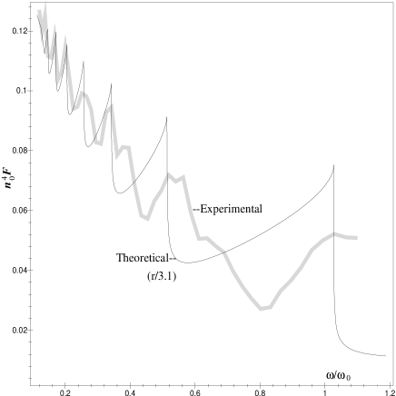
FIG. 3.: Comparison of the theoretical and experimental threshold amplitudes for $50\%$ ionization vs. $\omega/\omega_{0}$.

The shift in the position of the resonances from the integer fractional values seen in Fig. 2, due to the finite value of $r$, was approximated in Fig. 3 using the average value of $r$ over the range, $r\approx 0.195$.

In Figure 4 we plot $|\theta(t)|^{2}$ vs. $r$ for a fixed $t$ and two different values of $\omega$. These frequencies are chosen to correspond to the values of $\omega/\omega_{0}$ in the experimental curves. Figure 1 in [11] and Figure 1b in [3]. The agreement is very good for $\omega/\omega_{0}\approx.1116$ and reasonable for the larger ratio. Our model essentially predicts that when the fields are not too strong, the experimental survival curves for a fixed $n_{0}^{3}\omega$ (away from the resonances) should behave essentially like $\displaystyle\exp\left(-C[n^{4}_{0}F]^{\scriptstyle\frac{\scriptstyle 2}{\scriptstyle n_{0}^{3}\omega}}\,\,t\omega\right)$ with $C$ depending on $n_{0}^{3}\omega$ but, to first approximation, independent of $n_{0}^{4}F$.

The degree of agreement between the behavior of what might be considered as the absolutely simplest quantum mechanical model of a bound state coupled to the continuum and experiments on hydrogen atoms is truly surprising. The experimental results and in particular the resonances have often been interpreted in terms of classical phase space orbits in which resonance stabilization is due to KAM–like stability islands [3]. Such classical analogs are absent in our model as in fact are “photons”. On the other hand, the special nature of the edge of the continuum seems to be quite general, cf. [6].

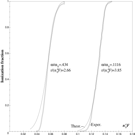
FIG. 4.: Ionization fraction at fixed $t$ (corresponding to 300 oscillations) as a function of amplitude.

We note that for $\omega>\omega_{0}$, in the limit of small amplitudes $r$, a predominantly exponential decay of the survival probability followed by a power-law decay was proven in [7] for three dimensional models with quite general local binding potentials having one bound state, perturbed by a local potential of the form $r\cos(\omega t)V_{1}(y)$. It seems likely that our results for general $\omega$ and $r$, including general periodic (perhaps also quasi-periodic) perturbations would extend to a similarly general setting. We are currently investigating various extensions of our model to understand the effect of the restriction to one bound state. This will hopefully lead to a more detailed understanding, and some control over the ionization process.

Because $\Gamma$ relates to the position of the poles of the solution of (8), a convenient way to determine $\Gamma$ (mathematical rigor aside), if $r$ is not too large, is the following, see also [6]. One iterates $n$ times the functional equation (8), $n$ appropriately large, to express $y(p)$ only in terms of $y(p\pm mi\omega)$ with $|m|>n$. After neglecting the small contributions of the $y(p\pm mi\omega)$, the poles of $y(p)$ can be obtained by a rapidly converging power series in $r$, whose coefficients are relatively easy to find using a symbolic language program, although a careful monitoring of the square-root branches is required. A complete study of the poles and branch-points of $y$ leads to (10) which is effectively the Borel summation of the formal (exponential) asymptotic expansion of $Y$ for $t\rightarrow\infty$.

Acknowledgments. We thank A. Soffer, M. Weinstein and P. M. Koch for valuable discussions and for providing us with their papers. We also thank R. Barker, S. Guerin and H. Jauslin for introducing us to the subject. Work of O. C. was supported by NSF Grant 9704968, that of J. L. L. and A. R. by AFOSR Grant F49620-98-1-0207.

* Also Department of Physics.

costin@math.rutgers.edu, lebowitz@sakharov.rutgers.edu, rokhlenk@math.rutgers.edu.

REFERENCES

- [1] Atom-Photon Interactions, by C. Cohen-Tannoudji, J. Duport-Roc and G. Arynberg, Wiley (1992).
- [2] P. T. Greenland, Nature 387, 548 (1997).
- [3] P. M. Koch and K.A.H. van Leeuwen, Physics Reports 255, 289 (1995).
- [4] R. M. Potvliege and R. Shakeshaft, Phys. Rev. A 40, 3061 (1989).
- [5] G. Scharf, K.Sonnenmoser, and W. F. Wreszinski, Phys.Rev. A, 44, 3250 (1991); S. Geltman, J. Phys. B: Atom. Molec. Phys., 5, 831 (1977).
- [6] S. M. Susskind, S. C. Cowley, and E. J. Valeo, Phys.Rev. A, 42, 3090 (1994).
- [7] A. Soffer and M. I. Weinstein, Jour. Stat. Phys. 93, 359–391 (1998).
- [8] S. Guerin and H.-R. Jauslin, Phys. Rev. A 55, 1262 (1997) and references there; E. V. Volkova, A. M. Popov, and O.V.Tikhonova, Zh. Eksp. Teor. Fiz. 113, 128 (1998).
- [9] A. Rokhlenko and J. L. Lebowitz, preprint (1998).
- [10] O. Costin, J. L. Lebowitz and A. Rokhlenko (in preparation).
- [11] P. M. Koch, Acta Physica Polonica A, 93 No. 1, 105–133 (1998).