The recursive adaptive quadrature in MS Fortran-77

Abstract

It is shown that MS Fortran-77 compilers allow to construct recursive subroutines. The recursive one-dimensional adaptive quadrature subroutine is considered in particular. Despite its extremely short body (only eleven executable statements) the subroutine proved to be very effective and competitive. It was tested on various rather complex integrands. The possibility of function calls number minimization by choosing the optimal number of Gaussian abscissas is considered.

The proposed recursive procedure can be effectively applied for creating more sophisticated quadrature codes (one- or multi-dimensional) and easily incorporated into existing programs.

1 Introduction

As it was shown in [10, 11] the application of recursion makes it possible to create compact, explicit and effective integration programs. In the mentioned papers the C++ version of such a routine is presented. However, it is historically formed that a large number of science and engineering Fortran-77 codes have been accumulated by now in the form of applied libraries and packages. That is one of the reasons why Fortran-77 is still quite popular in the applied programming. From this standpoint it seems to be very useful to use such an effective recursive integration algorithm in Fortran-77. There exist at least two possibilities to realize it. The first one is described in [10] where the interface for calling mentioned C++ recursive integration function from MS Fortran-77 is presented. The second possibility consist in constructing the recursive subroutine by means of Fortran-77 only. This is the particular subject of the paper where the possibility and benefits of recursion strategy in MS Fortran-77 is discussed.

2 Recursion in MS Fortran-77

The direct transformation of the mentioned C++ code is not possible mainly due to the formal inhibition of the recursion in Fortran-77. However, Microsoft extensions of Fortran-77 (e.g. MS Fortran V.5.0, Fortran Power Station) allow to make indirect recursive calls. It means that subprogram can call itself through intermediate subprogram. If anybody doubts he can immediately try:

call rec(1.0)

end

subroutine rec(hh)

integer i/0/

i = i + 1

h = 0.5*hh

write(*,*) i, h

if (i.lt.3) call mediator(h)

write(*,*) i, h

end

subroutine mediator(h)

call rec(h)

end

and get the following results:

1	5.000000E-01
2	2.500000E-01
3	1.250000E-01
3	1.250000E-01
3	1.250000E-01
3	1.250000E-01

But this is not a true recursion because no mechanism is supplied for restoring the values of the internal variables of the subroutine after its returning from recursion. The last requirement can be fulfilled by the forced storing of the internal variables into the program stack. The AUTOMATIC description of variables provides such possibility in MS Fortran-77. Taking this into account, the above example can be rewritten:

call rec(1.0)

end

subroutine rec(hh)

integer i/0/

automatic h, i

i = i + 1

h = 0.5*hh

write(*,*) i, h

if (i.lt.3) call mediator(h)

write(*,*) i, h

end

subroutine mediator(h)

call rec(h)

end

that yields:

1	5.000000E-01
2	2.500000E-01
3	1.250000E-01
3	1.250000E-01
3	2.500000E-01
3	5.000000E-01

Here the values of h are restored after each returning from recursion because it is saved in the stack before the recursive call. Note, that although the i variable is described as AUTOMATIC nonetheless its value is not saved.

3 Recursive adaptive quadrature algorithm

The described possibilities allow to employ effective recursion strategy for creating adaptive quadrature subroutine in MS Fortran-77.

The presented algorithm consists of two independent parts: adaptive subroutine and quadrature formula. The adaptive subroutine uses recursive algorithm to implement standard bisection method (see fig.1). For reaching desired relative accuracy $\varepsilon$ of the integration the integral estimation $I_{whole}$ over [$a_{i}$,$b_{i}$] subinterval on the i-th step of bisection is compared with the sum of $I_{left}$ and $I_{right}$ integral values that are evaluated over left and right halves of the considered subinterval. The comparison rule was chosen in the form:

$$I_{left}+I_{right}-I_{whole}\leq\varepsilon\cdot I,$$ (1)

where $I$ denotes the integral sum over whole integration interval [a,b]. The value of $I$ is accumulated and adjusted on each step of bisection.

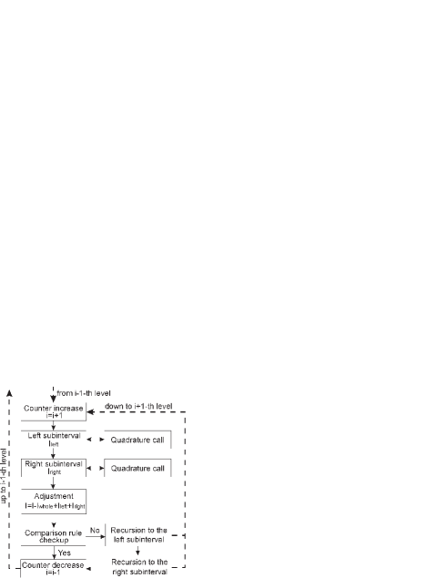
Figure 1: Adaptive recursive quadrature algorithm.

Should (1) be not fulfilled the adaptive procedure is called recursively for both (left and right) subintervals. Evaluation of the integral sums on each step of bisection is performed by means of quadrature formula. There are no restrictions on the type of quadratures used during integration. This makes the code to be very flexible and applicable to a wide range of integration problems.

The form (1) of the chosen comparison rule does not pretend on effectiveness rather on simplicity and generality. Really it seems to be very common and does not depend on the integrand as well as quadrature type. At the same time the use of (1) in some cases can result in overestimation of the calculated integral that consequently leads to more integrand function calls. One certainly can get some gains using, for instance, definite quadratures with different number or/and equidistant points or Gauss-Kronrod quadrature [7] etc. The comparison rule in the later cases becomes more effective but complex, intricate and sometimes less common. Whatever the case, the choice of comparison rule as well as the problems connected with it lie outside the subject of the publication.

Let us note some advantages which the application of the recursive call ideology to numerical integration can reveal:

• Very simple and evident algorithm that could result in extremely short as well as easy for further modifications and possible enhancements adaptive code.

• Because of the indicated shortness the adaptive procedure’s own running time has to be diminutive. That could result in its better performance compared to the known programs especially in the cases when the integrand function calculations are not time consuming.

• There is no need to store the integrand function values and pay attention on their correct usage. Besides no longer the control of subinterval bounds is in need. Indicated features permit utmost reduction of the efforts that one has to pay while creating the adaptive code.

• Nothing but program’s stack size sets the restriction on the number of subintervals when the recursive procedure is used (see next section). At the same time for the existing programs the crush level of the primary interval is strictly limited by the dimensions of the static arrays.

4 Program realization

Fortran-77 version of adaptive subroutine practically coincides with the corresponding C++ QUADREC (Quadrature used Adaptively and Recursively) function [10]:

SUBROUTINE Quadrec(Fun,Left,Right,Estimation)
real*8 Fun, Left, Right, Estimation
real*8 Eps, Result, Section, SumLeft, SumRight, QuadRule
integer*4 RecMax, RecCur, RawInt
common /IP/ Eps, Result, RecMax, RawInt, RecCur
automatic SumLeft, SumRight, Section
external Fun
RecCur = RecCur+1
if (RecCur.le.RecMax) then
  Section = 0.5d0*(Left+Right)
  SumLeft = QuadRule(Fun,Left,Section)
  SumRight = QuadRule(Fun,Section,Right)
  Result = Result+SumLeft+SumRight-Estimation
  if (dabs(SumLeft+SumRight-Estimation).gt.Eps*dabs(Result)) then
    call Mediator(Fun,Left,Section,SumLeft)
    call Mediator(Fun,Section,Right,SumRight)
  end if
else
  RawInt = RawInt+1
end if
RecCur = RecCur-1
return
end

Note that subroutine contains only eleven executable statements. The integrand function name, left and right bounds of the integration interval as well as the initial estimation of the integral value are the formal arguments of the subroutine. The IP common block contains the following variables: desired relative accuracy (Eps), the result of the integration (Result), maximum and current levels of recursion (RecMax, RecCur) as well as raw (not processed during integration) subintervals (RawInt).

The Section variable is used for storing a value of midpoint of the current subinterval. The integral sums over its left and right halves are estimated by QuadRule external function and stored in LeftSum and RightSum variables. The last three variables are declared as AUTOMATIC allowing to preserve their values from changing and use them after returning from recursion.

Execution of the subroutine begins with increasing of recursion level counter. If its value does not exceed RecMax, the integral sums over left and right halves of the current subinterval are evaluated, the integration result is updated and accuracy of the integration is checked. If achieved accuracy is not sufficient then subprogram calls itself (with the help of mediator subroutine) over left and right halves of subinterval. In the case the accuracy condition is satisfied the recursion counter decreases and subprogram returns to the previous level of recursion. The number of raw subintervals is increased when desired accuracy is not reached and RecCur is equal to RecMax.

The mediator subroutine has only one executable statement:

      subroutine Mediator(Fun,Left,Right,Estimation)
      real*8 Estimation, Fun, Left, Right
      external Fun
      call Quadrec(Fun,Left,Right,Estimation)
      return
      end

The main part of the integration program can be look like:

      common   /IP/ Eps, Result, RecMax, RawInt, RecCur
      common   /XW/ X, W, N
      integer  RecMax, RawInt, RecCur
      real*8   X(100), W(100), Left/0.0d0/, Right/1.0d0/
      real*8   Result, Eps, QuadRule
      real*8   Integrand
      external Integrand
      Eps = 1.0d-14
      N = 10
      RecCur = 0
      RecMax = 10
      call gauleg(-1.0d0,1.0d0,X,W,N)
      Result = QuadRule(Integrand,Left,Right)
      call Quadrec(Integrand,Left,Right,Result)
      write(*,*) ’ Result = ’,Result,’  RawInt = ’,RawInt
      end

The common block XW contains Gaussian abscissas and weights which are calculated with the help of gauleg subroutine for a given number of points N. The text of subroutine, reproduced from [8], is presented in Appendix A.

The text of QuadRule function is presented below:

      real*8 function QuadRule(Integrand,Left,Right)
      common /XW/ X, W, N
      real*8 X(100),W(100),IntSum,Abscissa,Left,Right,Integrand
      IntSum = 0.0d0
      do 1 i = 1, N
      Abscissa = 0.5d0*(Right+Left+(Right-Left)*X(i))
1     IntSum = IntSum + W(i)*Integrand(Abscissa)
      QuadRule = 0.5d0*IntSum*(Right-Left)
      return
      end

It is important to note that the number of recursive calls is limited by the size the program stack. This fact obviously sets the limit on the reachable number of the primary integration interval bisections and consequently restricts the integration accuracy. Note that stack size of the program can be enlarged by using /Fxxxx option of MS Fortran-77 compiler.

5 Numerical tests

The program testing was performed on four different integrals. In each case the exact values can be found analytically. That made it possible to control the desired and reached accuracy of the integration. Besides the same integrals were obtained with the help of well-known adaptive program QUANC8 reproduced from [4]. It allowed to compare the number of integrand function calls and the number of raw intervals for both programs.

The presented comparison has merely the aim to show that the use of recursion allows to construct very short and simple adaptive quadrature code that is not inferior to such a sophisticated program as QUANC8. Meanwhile the direct comparison of these programs seems to be incorrect because of a number of reasons.

The Newton-Cotes equidistant quadrature formula which is used in QUANC8 allows to make reuse of integrand function values calculated in the previous steps of bisection. That is the reason why QUANC8 has to have higher performance in integrand function calls compared to adaptive programs that use quadratures with non-equidistant points. Since QUADREC is not oriented on the use of definite but any quadrature formula it can be specified as a program of the later type.

At the same time QUANC8 gives bad results for functions with unlimitedly growing derivative and does not work at all for functions that go to infinity at the either of the integration interval endpoints. There are none of the indicated restrictions in QUADREC. Furthermore the opportunity of choosing of quadrature type makes it to be a very flexible tool for integration. Here QUADREC gives a chance to choose quadrature which is the most appropriate to the task (see Section 6).

For integrals in sections 5.1 and 5.2 the optimal numbers of quadrature points were found and used for integration. The 24-point quadrature was applied for integration in sections 5.3 and 5.4.

5.1 Sharp peaks at a smooth background

Let us start with the calculation of the integral cited in [4]:

$$\int\limits_{0}^{1}\left(\frac{1}{(x-a_{1})^{2}+a_{2}}+\frac{1}{(x-b_{1})^{2}+b_{2}}-c_{0}\right)dx$$ (2)

The integrand is the sum of two Lorenz type peaks and a constant background. At the beginning, values of $a_{1}$, $a_{2}$, $b_{1}$, $b_{2}$ and $c_{0}$ parameters were chosen to be the same as in the cited work. Then test was conducted at decreasing values of $a_{2}$ and $b_{2}$, which determine width of the peaks, while both programs satisfied desired accuracy and did not signal about raw subintervals. The results of the test when $a_{2}=b_{2}=10^{-8}$ are presented in Table 1. Note that only the optimal values are given for QUADREC program. The corresponding optimal numbers of Gaussian quadrature points are indicated.

Table 1: Testing results for integral (2).

Desired	QUANC8		QUADREC
relative	Number of	Reached	Number of	Reached	Optimal
accuracy	function calls	accuracy	function calls	accuracy	quadrature
1.0e-4	433	5.8e-06	665	3.7e-08	7
1.0e-5	513	1.5e-06	721	3.8e-08	7
1.0e-6	641	5.0e-07	792	3.2e-09	8
1.0e-7	801	7.2e-08	952	4.6e-10	8
1.0e-8	993	2.8e-09	1080	1.6e-10	8
1.0e-9	1217	2.1e-10	1304	8.8e-13	8
1.0e-10	1521	4.6e-11	1399	2.4e-14	13
1.0e-11	1825	6.5e-12	1599	4.4e-15	13
1.0e-12	2337	1.3e-13	1807	2.9e-16	13
1.0e-13	2945	1.4e-14	1859	1.1e-18	13
1.0e-14	3665	8.1e-16	1911	4.3e-19	13

As it follows from the given data the number of integrand function calls are compared for the both programs in the wide range of desired accuracy. Meanwhile it is interesting to point the attention on the fact that the use of optimal quadratures can give definite profits in the reached accuracy and number of integrand function calls even when the simple comparison rule (1) and no reuse of the integrand values are applied.

At further decreasing of $a_{2}$ and $b_{2}$ parameters QUANC8 informed about raw intervals and did not satisfy desired accuracy. At the same time QUADREC gave correct results for the integral down to parameter values $a_{2}=b_{2}=10^{-19}$. This is mainly due to the differences between static and dynamic memory allocation ideologies which are used in QUANC8 and QUADREC respectively.

5.2 Integration at a given absolute accuracy

The next test concerns the integration of the function:

$$f(x)={(1-\alpha x)\exp(-\alpha x)\over x^{2}\exp(-2\alpha x)+b^{2}}$$ (3)

over whole positive real axes. It is easy to show that its exact value is equal to zero. For reducing the integration interval to [0,1] the evident substitution x=t/(1-t) was used. As far as absolute accuracy of the integration was required the fourteenth line in the listed above QUADREC function text was changed to:

if (dabs(SumLeft+SumRight-Estimation).gt.Eps) then

The results of the test are presented in Table 2.

Table 2: Testing results for integrand (3).

Desired	QUANC8		QUADREC
absolute	Number of	Reached	Number of	Reached	Optimal
accuracy	function calls	accuracy	function calls	accuracy	quadrature
10e-5	33	1.1e-06	44	-3.7e-07	4
10e-6	33	1.1e-06	55	-7.1e-08	5
10e-7	49	1.1e-07	75	-1.1e-10	5
10e-8	49	1.1e-07	95	-3.5e-13	5
10e-9	65	6.1e-11	114	-1.9e-14	6
10e-10	81	1.7e-13	114	-1.9e-14	6
10e-11	81	1.7e-13	133	-2.2e-16	7
10e-12	145	-5.6e-14	152	-4.2e-18	8
10e-13	161	1.4e-15	152	-4.2e-18	8
10e-14	193	6.7e-16	190	-1.1e-19	10
10e-15	241	-3.4e-17	209	-1.2e-19	11
10e-16	305	-3.0e-17	230	-8.1e-20	10
10e-17	353	-7.3e-19	253	-1.2e-19	11
10e-18	513	4.1e-19	266	-2.8e-20	14

5.3 Improper integral

The next integrand function:

$$f(x)=x^{\frac{1}{n}-1}$$ (4)

becomes nonintegrable in the [0,1] interval when n goes to infinity. Besides function 4 goes to infinity at the low integration limit. That is the reason why QUANC8 can not be directly applied to the problem. To have still the opportunity of comparison, the integration of indicated function was performed from $10^{-10}$ to 1. The results of the test for number n up to and including 20 and desired relative accuracy of $10^{-14}$ are listed in Table 3. The second and fifth columns give the number of intervals that were not processed during the integration by both routines. The number of integrand function calls and values of reached relative accuracy are also presented in the table.

Table 3: Testing results for integration of (4) over [$10^{-10}$,1].

	QUANC8			QUADREC
n	Raw	Number of	Reached	Raw	Number of	Reached
	intervals	function	accuracy	intervals	function	accuracy
		calls			calls
1	0	33	0.0e+00	0	72	5.4e-20
2	14	2033	6.3e-10	0	2856	1.7e-18
3	22	2513	3.3e-08	0	2952	1.1e-16
4	50	3329	2.1e-07	0	2952	2.6e-18
5	70	3793	6.0e-07	0	2952	2.1e-16
6	74	3873	1.2e-06	0	2952	2.1e-16
7	108	4017	1.9e-06	0	2952	2.8e-16
8	130	4049	2.6e-06	0	2952	3.1e-18
9	150	4113	3.4e-06	0	2952	3.3e-16
10	146	4113	4.2e-06	0	2952	1.5e-16
11	164	4081	4.9e-06	0	3048	2.4e-16
12	176	4097	5.6e-06	0	3048	2.8e-16
13	164	4113	6.2e-06	0	3048	4.1e-16
14	184	4097	6.8e-06	0	3048	2.9e-16
15	200	4129	7.4e-06	0	3048	1.4e-16
16	166	4097	7.9e-06	0	3048	2.8e-18
17	187	4113	8.4e-06	0	3048	1.1e-16
18	182	4161	8.8e-06	0	3048	1.9e-16
19	184	4113	9.3e-06	0	3048	4.5e-16
20	156	4097	9.7e-06	0	3048	4.4e-16

Such a low performance of QUANC8, as it follows from the given data, can be explained by the type of comparison rule which it exploits. Really it is not applicable to functions like 4 that have unlimitedly growing derivative in some point(s) of integration interval.

The results of integration over whole interval [0,1] by QUADREC are shown in Table 4. The last column contains the maximum recursion level needed to achieve the desired accuracy. As far as it turned out to be a rather big the program stack size was correspondingly increased.

Table 4: Testing results for integration of (4) over [0,1].

n	Raw	Number of	Reached	Maximum
	intervals	function calls	accuracy	recursion level
1	0	72	0.0e+00	1
2	0	6504	1.0e-12	68
3	0	10344	1.1e-12	108
4	0	14088	1.2e-12	147
5	0	17928	1.2e-12	187
6	0	21672	1.3e-12	226
7	0	25416	1.3e-12	265
8	0	29256	1.3e-12	305
9	0	33000	1.3e-12	344
10	0	36744	1.4e-12	383
11	0	40584	1.3e-12	423
12	0	44328	1.4e-12	462
13	0	48072	1.4e-12	501
14	0	51912	1.4e-12	541
15	0	55656	1.4e-12	580
16	0	59400	1.4e-12	619
17	0	63240	1.4e-12	659
18	0	66984	1.4e-12	698
19	0	70728	1.4e-12	737
20	0	74568	1.4e-12	777

5.4 Evidence of program adaptation

Finally, integration of:

$$f(x)=sin(Mx)$$ (5)

over [0,2$\pi$] interval is appropriate for demonstrating the ability of an integration routine for adaptation. The exact integral value evidently is equal to zero for any integer M.

During the test a number of large simple integers were assigned to M and absolute integration accuracy of $10^{-10}$ was required. The output of the test is presented in Table 5. The accommodation of the routine evidently follows from the data. Namely, for M’s going from $\approx 10^{5}$ to $\approx 1.2\cdot 10^{6}$ the maximum recursion level (integrand function call number) changes from 15 ($\approx 1.6\cdot 10^{6}$) to 18 ($\approx 1.2\cdot 10^{7}$).

For all chosen values of M the desired accuracy was fulfilled. Furthermore program succeeded down to the accuracy of $10^{-12}$. Note that the standard stack size was used during the test and higher performance of the QUADREC certainly could be reached had the stack size been enlarged.

Table 5: Testing results for integrand (5).

n	Maximum	Number of	Reached absolute
	recursion level	integrand calls	accuracy
100003	15	1572840	3.2e-14
200003	16	3145704	-7.2e-14
300007	16	3145704	7.0e-15
400009	17	6290664	1.9e-14
500009	17	6291432	-2.2e-14
600011	17	6291432	-5.7e-15
700001	17	12364392	1.3e-15
800011	18	12580200	1.0e-13
900001	18	12582888	9.7e-14
1000003	18	12582888	2.2e-13
1100009	18	12582888	2.4e-15
1200007	18	12582888	-9.4e-14

6 The optimal quadrature

Here we want to take note of the possibility to minimize number of integrand calls by choosing the quadrature with optimal number of abscissas. The fig.2 demonstrates such a possibility.

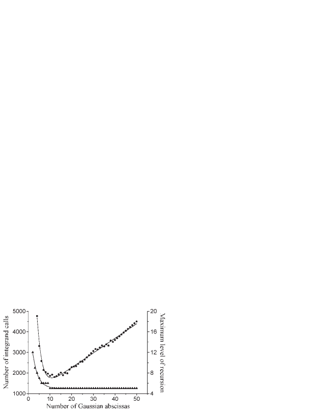
Figure 2: Number of integrand calls (circles) and maximum recursion level (triangles) versus the number of Gaussian abscissas.

Particularly, circles present the number of integrand calls versus the number of Gaussian abscissas used for the integration of 2 over [0,1] and desired relative accuracy of $10^{-10}$ and $a_{1}=0.3$, $a_{2}=10^{-9}$, $b_{1}=0.9$, $b_{2}=4.0\cdot 10^{-9}$, $c_{0}=6$. From the presented data one can see that the optimal number of Gaussian abscissas ranges approximately from 7 to 17. The use of more Gaussian abscissas leads to the linear growth of the number of function calls, because it does not result in essential reduction of the integration interval fragmentation. From the other hand the use of less number of Gaussian abscissas results in the significant growth of the number of function calls due to the extremely high fragmentation required. Dependence of the maximum recursion level upon the number of abscissas, presented by triangles, confirms this consideration.

Note that despite significant differences of the testing integrals (2,3) the optimal number of Gaussian abscissas turned out to be in the above limits.

7 Conclusion

Thus, the indirect recursion combined with AUTOMATIC variable description allow to employ true recursion mechanism in MS Fortran-77. In particular, the recursion strategy was applied to create effective adaptive quadrature code. Despite the simplicity and extremely small program body it showed good results on rather complex testing integrals. The created subroutine is very flexible and applicable to a wide range of integration problems. In particular, it was applied for constructing effective Hilbert transformation program. The last one was used to restore frequency dependence of refraction coefficient in analysis of optical properties of complex organic compounds. The subroutine can be easily incorporated into existing Fortran programs. Note that the coding trick, described in the paper, is very convenient for constructing multidimensional adaptive quadrature programs.

8 Acknowledgments

We express our thanks to Dr.V.K.Basenko for stimulating and useful discussion of the problem.

Appendix

A Guass-Legendr weights and quadratures

      subroutine gauleg(x1,x2,x,w,n)
      integer n
      real*8 x1,x2,x(n),w(n)
      real*8  eps
      parameter (eps=3.d-14)
      integer i,j,m
      real*8  p1,p2,p3,pp,xl,xm,z,z1
      m=(n+1)/2
      xm=0.5d0*(x2+x1)
      xl=0.5d0*(x2-x1)
      do 12 i=1,m
        z=cos(3.141592654d0*(i-.25d0)/(n+.5d0))
1       continue
          p1=1.d0
          p2=0.d0
          do 11 j=1,n
            p3=p2
            p2=p1
            p1=((2.d0*j-1.d0)*z*p2-(j-1.d0)*p3)/j
11        continue
          pp=n*(z*p1-p2)/(z*z-1.d0)
          z1=z
          z=z1-p1/pp
        if(abs(z-z1).gt.eps)goto 1
        x(i)=xm-xl*z
        x(n+1-i)=xm+xl*z
        w(i)=2.d0*xl/((1.d0-z*z)*pp*pp)
        w(n+1-i)=w(i)
12    continue
      return
      end

References

- [1] J.N.Lynnes, Comm. ACM 13(1970), p.260.
- [2] Genz and J.S.Chisholm, Computer PH 4(1972), p. 11 - 15.
- [3] Kahaner and M.B. Wells, SIAM Rev 18(1976), p. 811.
- [4] G.E.Forsythe,M.A.Malcolm,C.B.Moler, Computer methods for mathematical computations (Princeton Hall INC. 1977).
- [5] Lewellen, Computer Physics Communication 27(1982), p. 167 - 178.
- [6] Corliss and L.B Rall, SIAM J SCI 8(1987), p.831 - 847.
- [7] Kronrod A.S.,1964. Doklady Akdemii Nauk SSSR, vol. 154, p. 283-286.
- [8] W.H.Press, S.A.Teukolsky, W.T.Vetterling, B.P.Flannery. Numerical recipes in Fortran.
- [9] J.Mathews, R.L.Walker. Mathematical methods of physics. W.A. Benjamin, INC. 1964.
- [10] A.N.Berlizov, A.A.Zhmudsky. The recursive one-dimensional adaptive quadrature code. Preprint Institute for Nuclear Research. Kyiv. 1998.
- [11] A.A.Zhmudsky. One class of integrals evaluation in magnet solitons theory. Preprint LANL. /9800312. 1998.