VERIFICATION OF A LOCALIZATION CRITERION FOR SEVERAL DISORDERED MEDIA

We analytically compute a localization criterion in double scattering approximation for a set of dielectric spheres or perfectly conducting disks uniformly distributed in a spatial volume which can be either spherical or layered. For every disordered medium, we numerically investigate a localization criterion, and examine the influence of the system parameters on the wavelength localization domains.

Key words : localization, disordered media, electromagnetic scattering

Number of figures: 20

May 1999

CPT-99/P.3815

anonymous ftp: ftp.cpt.univ-mrs.fr
Web address: www.cpt.univ-mrs.fr

I INTRODUCTION

Several works of Anderson on localization [1] have mostly been related to electrons transport in solids with random impureties. Wolfle [2] has proposed a diagrammatical treatment for the electronic localization in a bidimensional disordered medium. This formalism was extended to the electromagnetic waves in a volume of disordered medium [3], [4], where the impureties are modeled by dielectric spherical scatterers, and the role played by the backscattering mechanism in the energy localization was established. The physical basis of the localization is a consequence of the vanishing of diffusion coefficient of the electromagnetic wave energy, this condition was then called a localization criterion.

The purpose of this paper is to analytically determine several conditions on the parameters of some disordered systems (namely, the number of scatterers, their size, permittivity, geometry, the width of the medium) satisfying a localization criterion of the electromagnetic energy, and to show their influence on the wavelength localization domains [5]. We give the analytic expressions of the localization criterion for a spherical or layered medium made of dielectric spheres or perfectly conducting disks. We numerically determine the sets of parameters offering ranges in wavelength where the localization criterion is satisfied. More precisely, we compute the evolution of the range when we modify every parameter, and we show that the location and the bandwitdh of these ranges may be controlled by varying some characteristic parameters of the disordered system.

This paper is organized as follows. After the introduction, we recall in Section 2 the mathematical model used to describe the behaviour of the electromagnetic wave in a disordered medium, and the expression of a localization criterion. Then in Section 3, we derive analytically a localization criterion for several disordered media. In Section 4, we numerically compute the localization criterion for these media in order to determine localization domains, and we examine the influence of the system parameters on these localization domains. Computations with a multidipolar formulation are used for comparison with the theoretical model. Finally, Section 5 is devoted to the conclusions.

II THE MATHEMATICAL MODEL

We consider $N$ identical scatterers of relative permittivity $\bar{\bar{\epsilon_{s}}}(\omega)$ distributed in a spatial volume $V$. The location of scatterers is given by the vector $\overrightarrow{R_{p}},p\in[1,N]$. The background medium has a relative permittivity $\epsilon_{0}$. An incident electromagnetic plane wave of pulsation $\omega$, and wavevector $k_{0}=\displaystyle{\frac{\omega}{c}}\sqrt{\epsilon_{0}}$, interacts with the set of scatterers (figure 1).

The electric field $\overrightarrow{E}(\overrightarrow{r},\omega)$ at location $\overrightarrow{r}$ satisfies the Helmholtz equation

$$\Delta\overrightarrow{E}(\overrightarrow{r},\omega)+k^{2}\bar{\bar{\epsilon}}(\overrightarrow{r},\omega).\overrightarrow{E}(\overrightarrow{r},\omega)=0,$$ (1)

where $k=\displaystyle{\frac{\omega}{c}}$ is the wavevector in the vacuum, $\bar{\bar{\epsilon}}(\overrightarrow{r},\omega)$ is the second rank tensor associated with the relative permittivity of the medium, where the components are given by

$$\epsilon_{ij}(\overrightarrow{r},\omega)=\epsilon_{0}\delta_{ij}+\sum_{p=1}^{N}\big{(}\epsilon_{sij}(\omega)-\epsilon_{0}\delta_{ij}\big{)}\chi_{\overrightarrow{R_{p}}}(\overrightarrow{r}),$$ (2)

$\chi_{\overrightarrow{R_{p}}}(\overrightarrow{r})$ is the characteristic function of the $p^{th}$ scatterer

$$\chi_{\overrightarrow{R_{p}}}(\overrightarrow{r})=\begin{cases}1\quad\text{if $\overrightarrow{r}$ inside the scatterer,}\\ 0\quad\text{outside}.\end{cases}$$ (3)

We assume the scatterers homogeneous and isotropic, thus

$$\epsilon_{ij}(\overrightarrow{r},\omega)=\bigg{(}\epsilon_{0}+\sum_{i=1}^{N}\big{(}\epsilon_{s}(\omega)-\epsilon_{0})\chi_{\overrightarrow{R_{i}}}(\overrightarrow{r})\bigg{)}\delta_{ij},$$ (4)

so we can treat the relative permittivity of the medium as a function of $\overrightarrow{r}$ and $\omega$.

Then, we write the Helmholtz equation in a perturbative form

$$\Delta\overrightarrow{E}(\overrightarrow{r},\omega)+\big{[}k_{0}^{2}-\delta V(\overrightarrow{r})\big{]}\overrightarrow{E}(\overrightarrow{r},\omega)=0,$$ (5)

where $\delta V(\overrightarrow{r})=k^{2}(\epsilon_{0}-\epsilon_{s})\sum_{i=1}^{N}\chi_{\overrightarrow{R_{i}}}(\overrightarrow{r})$ is the potential function describing the perturbation of the incident wavevector.

A The Green’s formalism

In order to solve the Helmholtz Eq. (5), we first introduce the dyadic Green function $g_{ij}(\overrightarrow{r},\overrightarrow{r^{\prime}},\omega)$ [6] which determines the wave at location $\overrightarrow{r}$ generated by a pointlike current source located in $\overrightarrow{r^{\prime}}$. Its components satisfy the Helmholtz equation

$$\Delta g_{ij}(\overrightarrow{r},\overrightarrow{r^{\prime}},\omega)+\big{[}k_{0}^{2}-\delta V(\overrightarrow{r})\big{]}g_{ij}(\overrightarrow{r},\overrightarrow{r^{\prime}},\omega)=\delta_{ij}\delta(\overrightarrow{r}-\overrightarrow{r^{\prime}}).$$ (6)

The interest of introducing a dyadic Green function is to provide a generic formulation for the electromagnetic field behaviour.

This equation can be written in an integral form

$$g_{ij}(\overrightarrow{r},\overrightarrow{r}^{\prime},\omega)=g^{0}_{ij}(\overrightarrow{r}-\overrightarrow{r}^{\prime},\omega)+\sum_{k=1}^{3}\int g^{0}_{ik}(\overrightarrow{r}-\overrightarrow{r_{1}},\omega)\delta V(\overrightarrow{r_{1}})g_{kj}(\overrightarrow{r_{1}},\overrightarrow{r}^{\prime},\omega)d\overrightarrow{r_{1}},$$ (7)

where $g^{0}_{ij}(\overrightarrow{r}-\overrightarrow{r^{\prime}},\omega)$ is the dyadic Green function of the electromagnetic wave in the nonperturbated medium of relative permittivity $\epsilon_{0}$, which satisfies the equation

$$g^{0}_{ij}(\overrightarrow{r}-\overrightarrow{r}^{\prime})=\bigg{(}\delta_{ij}+\partial_{i}\partial_{j}\bigg{)}g^{0}(\overrightarrow{r}-\overrightarrow{r}^{\prime}),$$ (8)

and $g^{0}(\overrightarrow{r}-\overrightarrow{r}^{\prime})$ is the scalar Green function of the wave

$$g^{0}(\overrightarrow{r}-\overrightarrow{r}^{\prime},\omega)=-\frac{1}{4\pi}\frac{e^{i\ k_{0}|\overrightarrow{r}-\overrightarrow{r}^{\prime}|}}{|\overrightarrow{r}-\overrightarrow{r}^{\prime}|}.$$ (9)

We introduce the Green operators ${\mathcal{G}}$ and ${\mathcal{G}}^{0}$

$${\mathcal{G}}^{0}\quad :\quad\overrightarrow{\Psi}(r)\rightarrow\int\bar{\bar{g^{0}}}(r-r^{\prime})\overrightarrow{\Psi}(r^{\prime})dr^{\prime},$$ (10)

$${\mathcal{G}}\quad :\quad\overrightarrow{\Psi}(r)\rightarrow\int\bar{\bar{g}}(r,r^{\prime})\overrightarrow{\Psi}(r^{\prime})dr^{\prime}.$$ (11)

The dyadic Green functions are defined by the kernels of the operators. The operator $\delta V$ in Eq. (7) is defined as the multiplicative operator, and the direct product between two successive operators is written as a point.

Using this formalism, we can rewrite the integral equation like

$${\mathcal{G}}={\mathcal{G}}^{0}+{\mathcal{G}}^{0}.\delta V.{\mathcal{G}}.$$ (12)

B First moment of ${\mathcal{G}}$ - Self energy operator

1 Model of disordered medium

The calculation of the kernel of ${\mathcal{G}}$ using a perturbative expansion of (12) requires the knowledge of the $3N$ space coordinates relative to the location of scatterers. Due to their complexity, we introduce a statistical approach of the problem. We call $\rho_{N}(\overrightarrow{R_{1}}...\overrightarrow{R_{N}})$ the probability density of location of the $N$ scatterers in the medium [7], and we introduce the mathematical expection value or mean IE defined by

$${\hbox{I\kern-1.99997pt\hbox{E}}}\big{(}{\mathcal{G}}\big{)}:\overrightarrow{\psi}(\overrightarrow{r})\rightarrow\int_{V}{g}_{ij}(\overrightarrow{r}-\overrightarrow{r}^{\prime},\omega)\rho_{N}(\overrightarrow{R_{1}}...\overrightarrow{R_{N}})\Pi_{p=1}^{N}d\overrightarrow{R}_{p}\psi(\overrightarrow{r}^{\prime})d\overrightarrow{r}^{\prime},$$ (13)

where we average over the whole possible configurations of the disordered medium.

2 First moment of ${\mathcal{G}}$

From Eq. (12), (13) we obtain

$${\hbox{I\kern-1.99997pt\hbox{E}}}\big{(}{\mathcal{G}}\big{)}={\mathcal{G}}^{0}+{\mathcal{G}}^{0}{\hbox{I\kern-1.99997pt\hbox{E}}}\big{(}\delta V.{\mathcal{G}}\big{)}.$$ (14)

By introducing the self-energy operator $\Sigma$ [3], defined by

$$\Sigma={\hbox{I\kern-1.99997pt\hbox{E}}}\big{(}\delta V.{\mathcal{G}}\big{)}\big{[}{\hbox{I\kern-1.99997pt\hbox{E}}}\big{(}{\mathcal{G}})\big{]}^{-1},$$ (15)

we can rewrite (14) like a Dyson equation

$${\hbox{I\kern-1.99997pt\hbox{E}}}\big{(}{\mathcal{G}}\big{)}={\mathcal{G}}^{0}+{\mathcal{G}}^{0}\Sigma{\hbox{I\kern-1.99997pt\hbox{E}}}\big{(}{\mathcal{G}}\big{)}.$$ (16)

The definition (15) of $\Sigma$ is not in a convenient form to obtain a solution, because ${\hbox{I\kern-1.99997pt\hbox{E}}}\big{(}{\mathcal{G}}\big{)}$ is the unknown of the equation. So, in order to calculate $\Sigma$, we prefer to link it with the multiple scattering formalism [3]. If ${\mathcal{T}}$ is the scattering operator of the medium, ${\mathcal{T}}$ is defined by

$${\mathcal{G}}={\mathcal{G}}^{0}+{\mathcal{G}}^{0}.{\mathcal{T}}.{\mathcal{G}}^{0},$$ (17)

and the expectation value ${\hbox{I\kern-1.99997pt\hbox{E}}}({\mathcal{T}})$ of the scattering operator is given by

$${\hbox{I\kern-1.99997pt\hbox{E}}}({\mathcal{T}})={\mathcal{G}}^{0}+{\mathcal{G}}^{0}.{\hbox{I\kern-1.99997pt\hbox{E}}}({\mathcal{T}}).{\mathcal{G}}^{0}~{}.$$ (18)

We have the following relation between $\Sigma$ and ${\hbox{I\kern-1.99997pt\hbox{E}}}({\mathcal{T}})$,

$$\Sigma={\hbox{I\kern-1.99997pt\hbox{E}}}({\mathcal{T}})\bigg{[}1+{\mathcal{G}}^{0}.{\hbox{I\kern-1.99997pt\hbox{E}}}({\mathcal{T}})\bigg{]}^{-1}={\hbox{I\kern-1.99997pt\hbox{E}}}({\mathcal{T}})-{\hbox{I\kern-1.99997pt\hbox{E}}}({\mathcal{T}}).{\mathcal{G}}^{0}.{\hbox{I\kern-1.99997pt\hbox{E}}}({\mathcal{T}})+...,$$ (19)

where ${\mathcal{T}}$ can be expressed using a multiple scattering expansion in terms of the scattering operator by a single scatterer $t_{i}$ at location $\overrightarrow{R}_{i}$,

$${\mathcal{T}}=\sum_{i=1}^{N}t_{i}+\sum_{i=1}^{N}{t}_{i}{\mathcal{G}}^{0}\cdot\sum_{j=1,j\neq i}^{N}t_{j}+\sum_{i=1}^{N}t_{i}{\mathcal{G}}^{0}\cdot\sum_{j=1,j\neq i}^{N}t_{j}{\mathcal{G}}^{0}\cdot\sum_{k=1,k\neq j}^{N}t_{k}+...$$ (20)

The interest of the last expression is to express $\Sigma$ by the mean of a scattering theory instead of calculating it from a perturbative expansion.

3 Macroscopic homogenization of the disordered medium - Scalar formulation

We use the hypothesis of macroscopic homogenization of the disordered medium in order to calculate the kernel of ${\hbox{I\kern-1.99997pt\hbox{E}}}\big{(}{\mathcal{G}}\big{)}$, i.e., the dyadic Green function of the averaged wave. We suppose that after averaging, the medium behaves like a homogeneous one, which implies an invariance under translation. In consequence, we can first write the Dyson equation (16) like a convolution equation

$${\hbox{I\kern-1.99997pt\hbox{E}}}\big{(}{\mathcal{G}}\big{)}={\mathcal{G}}^{0}+{\mathcal{G}}^{0}*\Sigma*{\hbox{I\kern-1.99997pt\hbox{E}}}\big{(}{\mathcal{G}}\big{)}.$$ (21)

The other consequence of the macroscopic homogenization hypothesis is the possibility to write a scalar form of the previous equation. Indeed, the averaged medium being homogeneous, the kernel of ${\hbox{I\kern-1.99997pt\hbox{E}}}\big{(}{\mathcal{G}}\big{)}$ may be written as

$${\hbox{I\kern-1.99997pt\hbox{E}}}\big{(}g(\overrightarrow{r}-\overrightarrow{r}^{\prime})\big{)}_{ij}=\bigg{(}\delta_{ij}+\partial_{i}\partial_{j}\bigg{)}{\hbox{I\kern-1.99997pt\hbox{E}}}\big{(}g(\overrightarrow{r}-\overrightarrow{r}^{\prime})\big{)},$$ (22)

where ${\hbox{I\kern-1.99997pt\hbox{E}}}\big{(}g(\overrightarrow{r}-\overrightarrow{r}^{\prime})\big{)}$ is the first moment of the scalar Green function of the electromagnetic wave. The same consideration holds for the kernel of the self-energy operator. Extracting the scalar part of Eq. (21), we obtain the scalar expression of the Green function in Fourier space

$${\hbox{I\kern-1.99997pt\hbox{E}}}\big{(}G(\overrightarrow{k},\omega)\big{)}=\frac{1}{k^{2}-k_{0}^{2}-\Sigma(\overrightarrow{k},\omega)},$$ (23)

where we notice that the invariance by translation of the averaged medium implies that the first moment of the Green function and the self energy function in Fourier space are only $\overrightarrow{k}$ dependent. ${\hbox{I\kern-1.99997pt\hbox{E}}}(G)$ is the scalar Green function of the homogenized medium.

The argument of Sheng [4] is to treat the averaged medium like an effective medium, where the characteristic length of the averaged inhomogenities is small with respect to the wavelength, and therefore, they are not resolved by the wave, which explains that the averaged medium may be considered like a homogeneous one. In that case, the self-energy function $\Sigma$ describing the local microstructures of the medium, is weakly dependent on the variable $\overrightarrow{k}$, so it is treated like a pulsation dependent function $\Sigma(\omega)$.

If this condition is satisfied, the first moment of the Green function physically represents a propagative wave of effective wavevector ${\tilde{k}}_{e}^{2}=k_{0}^{2}+\Sigma(\omega)$, from which we deduce the wavevector of the wave

$$k_{e}=\mbox{Re}\big{(}{\tilde{k}}_{e}\big{)}=\sqrt{\frac{k_{0}^{2}+\Gamma}{2}}\bigg{[}1+\sqrt{1+\big{(}\frac{\gamma}{k_{0}^{2}+\Gamma}\big{)}^{2}}\bigg{]}^{\frac{1}{2}},$$ (24)

where $\Gamma=\mbox{Re}\big{(}\Sigma(\omega)\big{)}$, $\gamma=\mbox{Im}\big{(}\Sigma(\omega)\big{)}$, and the scattering length $l$ [3] which is the inverse of twice the damping rate $\beta$ of the modulus of the averaged wave

$$l=\frac{1}{2\beta}=\frac{k_{e}}{\gamma}.$$ (25)

The decreasing factor in the expression of the first moment of the Green function shows the fact that during the path in the averaged medium, the wave loses its phase coherence over a characteristic length given by $l$, as a consequence of the successive scatterings. Over a distance of several scattering lengths $l$, the first moment of the Green function becomes negligible. In order to describe the behaviour of the electromagnetic wave for large distances, we need to investigate the second moment of the dyadic Green function.

C The second moment of ${\mathcal{G}}$ - Localization of the energy

The averaged energy operator $\mathcal{P}$ is given by the averaged tensorial product of the two Green operators ${\mathcal{G}}$ and ${\mathcal{G}}^{*}$, where their kernels are respectively the dyadic Green function of the electromagnetic wave at pulsation $\omega_{+}=\omega+\displaystyle{\frac{\delta\omega}{2}}$ and the conjugate complex dyadic Green function at pulsation $\omega_{-}=\omega-\displaystyle{\frac{\delta\omega}{2}}$

$${\hbox{I\kern-1.99997pt\hbox{E}}}\big{(}\mathcal{P}\big{)}={\hbox{I\kern-1.99997pt\hbox{E}}}\big{(}{\mathcal{G}}\otimes{\mathcal{G}}^{*}\big{)},$$ (26)

where $\omega$ is the central pulsation of the two dyadic Green functions, and $\delta\omega$ is their pulsation difference. We notice that $\delta\omega$ is the conjugated variable of the time traject $t$ of the electromagnetic wave in the medium. The behaviour for $t\rightarrow+\infty$ of the averaged energy will be given by the behaviour of the kernel of ${\hbox{I\kern-1.99997pt\hbox{E}}}\big{(}\mathcal{P}\big{)}$ when $\delta\omega\rightarrow 0$.

The outer product $\otimes$ applied on the components of the dyadic Green functions is given by

$$\big{(}g\otimes g^{*}\big{)}_{ijkl}(\overrightarrow{r},\overrightarrow{r}^{\prime},\omega,\delta\omega)=g_{ij}(\overrightarrow{r},\overrightarrow{r}^{\prime},\omega_{+})g^{*}_{kl}(\overrightarrow{r},\overrightarrow{r}^{\prime},\omega_{-}).$$ (27)

Using the macroscopic homogenization hypothesis, we can write the scalar form of the kernel of ${\hbox{I\kern-1.99997pt\hbox{E}}}\big{(}\mathcal{P}\big{)}$, which is defined as the function ${\hbox{I\kern-1.99997pt\hbox{E}}}\big{(}P(\overrightarrow{r},\overrightarrow{r^{\prime}},\omega,\delta\omega)\big{)}$, and is related to the average energy density function $L$ by its spatial Fourier transform

$${\hbox{I\kern-1.99997pt\hbox{E}}}\big{(}P(\overrightarrow{r},\overrightarrow{r^{\prime}},\omega,\delta\omega)\big{)}=\frac{1}{2\pi}\int L(\overrightarrow{q},\omega,\delta\omega)e^{i\overrightarrow{q}.(\overrightarrow{r}-\overrightarrow{r^{\prime}})}d\overrightarrow{q}.$$ (28)

Let us remark that the $q$ variable in the function $L$ is conjugated with the wave traject $|\overrightarrow{r}-\overrightarrow{r}^{\prime}|$. The behaviour of the average energy at large distance will be given by the behaviour of $L$ when $q\rightarrow 0$.

Following the frameworks of Arya[3] and Sheng [4], at large distances ($q\rightarrow 0$) and large time ($\delta\omega\rightarrow 0$), $L$ is governed by a diffusion-like equation

$$-i\delta\omega L(\overrightarrow{q},\omega,\delta\omega)=q^{2}D(\overrightarrow{q},\omega,\delta\omega)L(\overrightarrow{q},\omega,\delta\omega),$$ (29)

where

$$D(\overrightarrow{q},\omega,\delta\omega)\!\!=D^{B}(\omega)\bigg{[}1-\frac{\pi}{3k_{e}^{2}l^{2}}\int_{Q=0}^{Q\sim\frac{1}{l}}{Q^{2}\over{i\delta\omega\over D(\bf q,\omega,\delta\omega)}+Q^{2}}dQ\bigg{]},$$ (30)

is the general energy diffusion coefficient of the wave, and

$$D^{B}(\omega)=\frac{\omega l}{3k_{e}},$$ (31)

is the Boltzmann diffusion coefficient. The corrective term involved in the general expression of the diffusion coefficient is a consequence of the backscattering effect of the electromagnetic wave in the disordered medium.

The energy of the electromagnetic wave is said to be localized when the general diffusion coefficient (30) vanishes, i.e. the corrective term generated by the backscattering compensates the Boltzmann diffusion coefficient, which gives us the condition

$$k_{e}.l\leq\sqrt{\frac{3}{\pi}},$$ (32)

$k_{e}$ and $l$ are given by the relations (24) and (25). This condition is called the localization criterion of the electromagnetic wave energy.

III Calculation of the localization criterion
for several media

We propose to derive an analytic expression of the localization criterion for an electromagnetic wave of wavelength $\lambda_{0}=\displaystyle{\frac{2\pi}{k_{0}}}$ interacting with the two following sets of media.

- A set of $N$ identical dielectric spheres of radius $a$ and relative permittivity $\epsilon_{s}$, uniformly distributed in a spherical volume $V$ , or in a layered volume of thickness $e_{z}$ (figure 2).

- A set of $N$ identical perfectly conducting disks of radius $a$ and relative permittivity $\epsilon_{s}$, uniformly distributed in a spherical volume $V$ , or in a layered volume of thickness $e_{z}$ (figure 3).

The definitions of the averaged wavevector $k_{e}$ and the scattering length $l$ are given by the relations (24) and (25). To express the $k_{e}.l$ product, we have to calculate the self-energy function for every disordered medium.

A Macroscopic homogenization conditions

First, we need to verify some conditions on the media in order to consider them as macroscopically homogeneous, which means that the self-energy function must be only $k$ dependent.

The self-energy function in Fourier space for a medium of $N$ identical scatterers of scattering function $t(\overrightarrow{k},\overrightarrow{k}^{\prime})$ is given by

$$\Sigma(\overrightarrow{k},\overrightarrow{k}^{\prime})=\frac{N}{V}t(\overrightarrow{k},\overrightarrow{k}^{\prime})\int_{V}e^{i(\overrightarrow{k}-\overrightarrow{k}^{\prime}).\overrightarrow{R}_{i}}d\overrightarrow{R}_{i},$$ (33)

where $V$ is the volume of the medium. The integral in (33) taken over a finite volume can be approximated as

$$\int_{V}e^{i(\overrightarrow{k}-\overrightarrow{k}^{\prime}).\overrightarrow{R}_{i}}d\overrightarrow{R}_{i}=\delta(\overrightarrow{k}-\overrightarrow{k}^{\prime})\quad\text{if}\begin{cases}\text{radius $R$ of the medium $>>\displaystyle{\frac{\lambda}{4}}$}\\ \text{thickness $e_{z}>>\displaystyle{\frac{\lambda}{2}}$}\end{cases}$$ (34)

which leads to the condition of macroscopic homogenization, because the delta distribution argument $\overrightarrow{k}^{\prime}-\overrightarrow{k}$ implies that the self-energy function is only $\overrightarrow{k}$ dependent.

B Calculation of $k_{e}$ and $l$

Using expansions (19) and (20), the first and the second scattering order of the self energy operator are respectively given by the following expressions

$$\Sigma={\hbox{I\kern-1.99997pt\hbox{E}}}\big{(}\sum_{i=1}^{N}t_{i}\big{)},$$ (35)

$$\Sigma={\hbox{I\kern-1.99997pt\hbox{E}}}\big{(}\sum_{i=1}^{N}t_{i}\big{)}-{\hbox{I\kern-1.99997pt\hbox{E}}}\big{(}\sum_{i=1}^{N}t_{i}.{\mathcal{G}}^{0}.t_{i}\big{)}.$$ (36)

By assuming the macroscopic homogenization hypothesis, we can derive the scalar expressions of the kernels. For the second scattering order, we suppose that every scatterer receives a wave being locally plane, in that case, the scalar part of the Green propagator simplifies to $g^{0}(\overrightarrow{k},\omega)=-i\pi\delta(k^{2}-k_{0}^{2})$. Since the $N$ scatterers are uniformly distributed in the volume $V$, we obtain

$$\Sigma(\omega)=\frac{N}{V}t(\omega)\quad\text{single scattering order},$$ (37)

$$\Sigma(\omega)=\frac{N}{V}t(\omega)+\pi\frac{N^{2}}{V^{2}}t^{2}(\omega)\quad\text{second scattering order},$$ (38)

where

$$V=\begin{cases}\frac{4}{3}\pi R^{3}\quad\text{for a spherical medium of radius $R$}\\ e_{x}.e_{y}.e_{z}\quad\text{for a layered volume of thickness $e_{z}$}\\ \text{and transverse widths $e_{x}$ and $e_{y}$}\end{cases}$$ (39)

$R$ or $e_{x}$, $e_{y}$ and $e_{z}$ must satisfy the conditions (34). The scattering functions are given by

$$t(\omega)=\begin{cases}\frac{2i\pi}{k_{0}}\sum_{p=1}^{+\infty}(2p+1)(a_{p}+b_{p})\\ \text{for a sphere of radius $a$ and permittivity $\epsilon_{s}$ \cite[cite]{[\@@bibref{Number}{Hulst}{}{}]}}\\ -k_{0}^{2}d\sqrt{2\pi}\bigg{(}\frac{16}{3}\big{(}\frac{k_{0}a}{2}\big{)}^{2}+\frac{512}{45}\big{(}\frac{k_{0}a}{2}\big{)}^{4}+i\frac{1024}{27\pi}\big{(}\frac{k_{0}a}{2}\big{)}^{5}\bigg{)}\\ \text{for a little disk of radius $a$ (d =2a) \cite[cite]{[\@@bibref{Number}{Nomura}{}{}]}}.\end{cases}$$ (40)

From (38), (39), (40), we obtain the expression of the averaged wavevector $k_{e}$ and the scattering length $l$ at the second scattering order.

- For $N$ spheres uniformly distibuted in a volume $V$

$$k_{e}=\frac{1}{\sqrt{2}}\sqrt{k^{2}+\frac{n}{2}\sum_{p=1}^{\infty}(2p+1)\mbox{Re}(a_{p}+b_{p})+\frac{n^{2}}{4}\big{(}\mbox{Re}(\sum_{p=1}^{\infty}(2p+1)(a_{p}+b_{p}))\big{)}^{2}\big{)}}\\ \bigg{[}1+\sqrt{1+\big{(}\frac{\frac{n}{2}\sum_{p=1}^{\infty}(2p+1)\mbox{Im}(a_{p}+b_{p})+\frac{n^{2}}{4}\big{(}\mbox{Im}(\sum_{p=1}^{+\infty}(2p+1)(a_{p}+b_{p})\big{)})^{2}}{k^{2}+\frac{n}{2}\sum_{p=1}^{\infty}(2p+1)\mbox{Re}(a_{p}+b_{p})+\frac{n^{2}}{4}\big{(}\mbox{Im}(\sum_{p=1}^{+\infty}(2p+1)(a_{p}+b_{p}))\big{)}^{2}}\big{)}^{2}}\bigg{]}^{\frac{1}{2}},$$ (41)

and

$$l=\frac{k_{e}}{\frac{n}{2}\sum_{p=1}^{\infty}(2p+1)\mbox{Im}(a_{p}+b_{p})+\frac{n^{2}}{4}\big{(}\mbox{Im}(\sum_{p=1}^{+\infty}(2p=1)(a_{p}+b_{p}))\big{)}^{2}}.$$ (42)

- For $N$ disks uniformly distributed in a volume $V$

$$k_{e} = \frac{1}{\sqrt{2}}\sqrt{k_{0}^{2}-2n\sqrt{2\pi}k_{0}^{2}d\mbox{Re}(D_{0}^{0})+8\pi n^{2}d^{2}k_{0}^{4}(\mbox{Re}(D_{0}^{0})^{2}}$$ (44)

$$\bigg{[}1+\sqrt{1+\big{(}\frac{-2n\sqrt{2\pi}k_{0}^{2}d\mbox{Im}(D_{0}^{0})+8\pi n^{2}d^{2}k_{0}^{4}\big{(}\mbox{Im}(D_{0}^{0})\big{)}^{2}}{k_{0}^{2}-2n\sqrt{2\pi}k_{0}^{2}d\mbox{Re}(D_{0}^{0})+8\pi n^{2}d^{2}k_{0}^{4}\big{(}(\mbox{Re}(D_{0}^{0})\big{)}^{2}}\big{)}^{2}}\bigg{]}^{\frac{1}{2}},$$

and

$$l=\frac{k_{e}}{-2n\sqrt{2\pi}k^{2}d\mbox{Im}(D_{0}^{0})+8\pi n^{2}d^{2}k_{0}^{4}\big{(}\mbox{Im}(D_{0}^{0})\big{)}^{2}},$$ (45)

where $D_{0}^{0}=\frac{16}{3}\big{(}\frac{k_{0}a}{2}\big{)}^{2}+\frac{512}{45}\big{(}\frac{k_{0}a}{2}\big{)}^{4}+i\frac{1024}{27\pi}\big{(}\frac{k_{0}a}{2}\big{)}^{5}$, and $n=N/V$ is the density.

IV Numerical results

A Characterization of the localization domains

We are now in position to search for localization domains, i.e, ranges of wavelength satisfying the localization criterion $k_{e}.l\leq\sqrt{\displaystyle\frac{3}{\pi}}$. In the following we have computed the $k_{e}.l$ product as a function of the incident wavelength $\lambda$, and labeled the localization curve as $k_{e}.l(\lambda)$. Then we will look for the influence of the system parameters on the localization, for instance: the number $N$, the width $a$ of the scatterers and for the case of spheres, their permittivity $\epsilon_{s}$, the volume $V$ of the medium. In our simulations, we have supposed that the relative permittivity $\epsilon_{s}$ is weakly dependent on the pulsation, so we have treated it as a scalar. However, it is possible to give a description by a frequency law dependent upon the nature of the scatterer. The calculations were performed using Mathematica .

The first medium we study is an array of $N$ dielectric spheres of radius $a$, permittivity $\epsilon_{s}$, uniformly distributed in a volume $V$ of radius $R$. We numerically found a localization domain for the following set of parameters (figure 4)

$N=$ 1 million
a = 0.01$\mu$
$\epsilon_{s}$=16
$R$ = 2$\mu$
$\lambda\in[0.0805\mu,0.083\mu]$. We satisfy the criteria of macroscopic homogenization of the medium because in that case the ratio $\displaystyle{\frac{R}{\lambda}}$ is about 25, and so the condition $\displaystyle{\frac{R}{\lambda}}>>\displaystyle{\frac{1}{4}}$ is valid. Let us notice that we are working in the range $k.a<1$, and only the first term of the expansion (40) was used in the calcultations of the scattering function for the spheres.

Now, we will investigate the effect of the parameters on the localization domain.

We show in figure 5, the localization curves for several values of the spheres radius. The dotted curve is taken for reference ($a=0.01\mu$). When the value of $a$ decreases (0.095$\mu$) (plain curve), the minimum of the curve occurs for lower wavelength, the corresponding value of the $k_{e}.l$ product increases and the localization domain narrows. Oppositely, when the radius is increased (0.0105$\mu$)(dashed curve), the minimum of the localization curve occurs for higher wavelength, the corresponding value of the $k_{e}.l$ product decreases and the localization domain enlarges.

In figure 6, we start from the reference configuration, and we modify the relative permittivity of spheres. The curves are shown for the values: $\epsilon=15$ (plain curve), $\epsilon=16$ (dotted curve) and $\epsilon=17$ (dashed curve). When we slightly increase the relative permittivity of the spheres, the localization domain enlarges with a translation to higher wavelengths.

Next, we have fixed the real part of the permittivity ($\mbox{Re}(\epsilon)=16$), and we simulate a absorption on the surface of spheres by adding an imaginary part to the relative permittivity, so we obtain a dissipative dielectric. The figure 7 shows the localization curves for the respective values 0 (plain curve), 0.4 (dotted curve), 0.8 (dashed curve) and 1.2 (long dashed curve) of the imaginary part of the relative permittivity. When the value of the imaginary part increases, the value of the minimum of the localization curve also increases and the localization domain narrows and finally disappear. By adding an imaginary part to the relative permittivity, the scatterers absorb a part of the electromagnetic energy and the interactions during successive scatterings are reduced, which explains the disappearance of localization.

An other interesting parameter is the density $n=\displaystyle{\frac{N}{V}}$. Indeed, when we increase the density of scatterers, we also increase the backscattering contributions from the successive interactions of the wave with scatterers, as a consequence the localization is more easily attained.

We verify the influence upon the number $N$ of scatterers in a fixed volume medium. The Figure 8 shows the localization curves corresponding to $N=1$ million (plain curve), $N=$1.5 millions (dotted curve) and $N=$2 millions (dash curve) spheres. When the number of scatterers increases, we observe a deepening of the localization curve minimum and a broadening of the localization domain. The inverse phenomenon was obtained when we fix the number of spheres and at the same time increase the radius of the medium. Figure 9 shows the localization curve for the radius $R$ values 2, 2.1, 2.2, 2.3, and 2.4 $\mu$ respectively. In that case, the minimum of the localization curve increases with $R$ and the localization domain disappears. The localization gradually vanishes because the medium is diluted, so the interactions between the scatterers are reduced. In both cases, the $N$ or $R$ variations show that the location of the minimums are weakly dependent, it means that one can choose a configuration giving a central vawelength localization, and then modify the width of the localization domain around this value by the mean of medium density.

In the next part, we only focuse on the density effect.

In the following example, we consider $N$ dielectric spheres uniformly distributed in a rectangular volume $[-\frac{e_{x}}{2},\frac{e_{x}}{2}]\times[-\frac{e_{y}}{2},\frac{e_{y}}{2}]\times[-\frac{e_{z}}{2},\frac{e_{z}}{2}]$, where $e_{x}$ and $e_{y}$ are large in front of $\lambda$ in order to approximate the rectangular medium by a single layer of thickness $e_{z}$.

We numerically found a localization domain for the set of parameters (figure 10)

$N=10^{5}$
a = 0.01$\mu$
$\epsilon_{s}$=16
thickness $e_{z}$ = 1.5 $\mu$
transverse lengths $e_{x}$=$e_{y}$=1.5 $\mu$
$\lambda\in[0.0805\mu,0.083\mu]$.

The figure 11 presents the localization curves when the number $N$ of spheres takes respectively the values: $10^{5}$ (plain curve), $1.210^{5}$ (dotted curve) and $1.510^{5}$ (dashed curve), the other parameters are kept fixed. We observe that the minimum of the curves diminishes with the increase of $N$ and the localization domain enlarges. Then, if we fix the number of spheres $N=10^{5}$, and modify the thickness $e_{z}$ of the layer with respect to the macroscopic homogenization condition. The figure 12 shows the curves obtained for $e_{z}=1\mu$ (plain curve), $e_{z}=1.5\mu$ (dotted curve) and $e_{z}=1.8\mu$ (dashed curve). The minimum of the curves increases with the thickness $e_{z}$ of the layer, the localization domain narrows and finally disappears. The observed effects are the same as in the case of a spherical volume.

In a second series of tests, we replace the spheres by perfectly conducting disks, oriented following a plane perpendicular to the wavevector (figure 3).

For the two respective media (spherical and layered), we numerically find a localization domain for the set of parameters in a spherical volume (figure 13),

$N=1$ billion
a = 0.05$\mu$
volume radius $R$ = 12.5$\mu$
$\lambda\in[0.45\mu,0.64\mu]$

and for a single layer (figure 14)

$N=150$millions
a = 0.05 $\mu$
thickness $e_{z}$ = 10 $\mu$
transverse lengths $e_{x}$=$e_{y}$=10 $\mu$
$\lambda\in[0.45\mu,0.74\mu]$.

Figures 15 and 16 show the localization curves for the spherical volume case when we vary respectively the number of disks and the radius of the volume. In figure 15, the volume radius is fixed, $R=15\mu$, and the number $N$ takes the values 1 billion (plain curve), 1.5 billions (dotted curve) and 2 billions (dashed curve), for this last value, the localization domain is located in the range [0.45 $\mu$, 0.72 $\mu$], it is larger compared to the case $N$=1.5 billion ([0.45 $\mu$, 0.60 $\mu$]). In figure 16, we have fixed $N$ at 1 billion and computed localization curves for $R$ = 10 $\mu$ (plain curve), $R$=12.5 $\mu$ (dotted curve), and $R$ = 15 $\mu$ (dashed curve). In the last case, the minimum of the localization curve is 1.1 for $\lambda=5\mu$, but there is no more localization.

The same effects occur in the case of a layered medium. When we increase the number of disks (figure 17) the localization domain enlarges, oppositely, when the thickness of the medium increases (figure 18), the localization range narrows and disappears.

B A Numerical check

In order to numerically control the behaviour of the electromagnetic field near a localization range, we have used a multidipolar diffusion formulation [10]. The principle consists to discretize a dielectric sphere of radius $a<\lambda$ by an array of dipoles [11], and to compute the scattered field using a multidipolar expansion. To characterize the scattered field, we use the intensity functions $I_{ij}(\theta)$ described in [12], where $i$ and $j$ respectively refer to the polarization of the incident and scattered electric field, $\theta$ is the scattering angle. More precisely, we are interested by the intensity behaviour around the backscattering direction, where the localization phenomenon manifests by the creation of a backscattering peak.

We compute the averaged intensity functions by supposing the disordered medium ergodic, which means that the mathematical expectation value of the intensity function is obtained by averaging intensity functions on a large number of disordered medium configurations.

Due to the large number of spheres we used for computations, we simplify the problem by modeling a little sphere by a single dipole located at its center.

C Case of a spherical volume

We first use the localization parameters previously obtained for the set of spheres in a spherical volume to compute the averaged intensity functions. In this model, a number of spheres around 1 million is too large to be handled by numerical computations. But we notice that the fundamental parameter which occurs in the localization criterion is the density $n=\displaystyle{\frac{N}{V}}$. To simulate an equivalent configuration, we define a medium of the same density but with a smaller number of spheres. However, the consequence is also to reduce the radius of the medium, and then alterate the macroscopic homogenization condition (34).

We choose the set of the following parameters: $R=0.2\mu$ and $N=1000$. The localization parameters are then

$N=1000$
a = 0.01 $\mu$
$\epsilon_{s}$=16
$R$ = 0.2 $\mu$
$\lambda\in[0.0805\mu,0.083\mu]$

We propose to compute the intensity functions for several values of $N$, when we approach a localization range (i.e., $N\rightarrow 1000$). Figure 19 shows the intensity functions $I_{xx}(\theta)$ (in arbitray units) for the respective values of $N$ =300,500,700,900. We notice the appearance of a peak in the backscattering direction when the value of $N$ approaches the theoretical value of $N$ given by the mathematical model ($N$=1000).

D Case of a layered medium

We use the localization parameters given for the set of spheres in a layered volume to compute the averaged intensity functions. Like in the previous example, the number of spheres is too large for a numerical computation. To overcome this difficulty, we use an equivalent medium with the same density.

We choose the set of equivalent parameters: $e_{x}=0.3\mu$, $e_{y}=0.3\mu$, $e_{z}=0.28\mu$ and $N=800$ . The localization parameters are then

$N=800$
$a=0.01\mu$
$\epsilon_{s}=16$
$e_{x}=e_{y}=0.3\mu$
$e_{z}=0.28\mu$
$\lambda\in[0.081\mu,0.083\mu]$

We present the intensity function curves $I_{xx}(\theta)$ when the number of spheres $N$ have respectively the values 200, 400, 600, 800 (figure 20). We also observe a backscattering peak when $N$ tends to the initial value where one observes an electromagnetic energy localization in the mathematical model.

V Conclusion and perspectives

We have analytically calculated the value of the $k_{e}.l$ product as a function of the incident wavelength in order to find wavelength domains satisfying the localization criterion $k_{e}.l\leq\displaystyle{\sqrt{\frac{3}{\pi}}}$ in different media. We have considered some configurations where the volume may be finite or infinite, and the scatterers are dielectric spheres or perfectly conducting little disks. We have studied the influence of electromagnetic system parameters on the localization domain, for instance, the complex permittivity of spheres, their radius, their number and the dimensions of the surrounding medium. Computations have shown that the density offers the optimal way to adjust the width of the localization domain.

The multidipolar model allowed us to detect a backscattering peak when the system parameters are closed to the localization parameters provided with the theoretical model. Many works were already realized in order to calculate the expression of the backscattering peak [4], [13], however these results were not related to the localization criterion. This peak, predicted by the theoretical model, occurs from the crossed diagrams contribution [2] responsible of the backscattering, it represents a first manifestation of the localization phenomenon. However, we were limited by the size of the matrix describing the system, and the conditions where the medium is macroscopically homogeneous were not exactly fulfilled. The same matrix limitation implies that we have, in the simulation, described a little sphere by a single dipole. A way to perform a more realistic simulation would consist to describe the sphere itself by a set of dipoles located on a cubic lattice inside the sphere [11].

VI Acknowledgements

C. O. thanks Thomson-CSF Optronique for a financial support during the preparation of his thesis. Contract CIFRE-400-95.

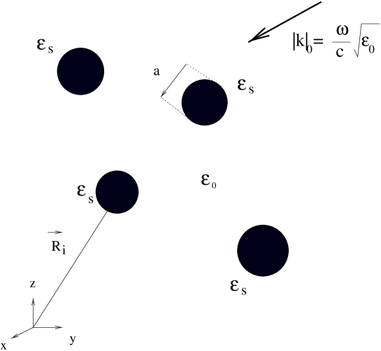
FIG. 1.: Scheme of the disordered medium.

     

FIG. 2.: Scheme for $N$ spheres uniformly distributed in a spherical volume or in a layered volume of finite thickness.

     

FIG. 3.: Scheme for $N$ disks uniformly distributed in a spherical volume or in a layered volume of finite thickness.

FIG. 4.: Localization curve for a set $N=$ 1 million spheres of radius $a=0.01\mu$, and relative permittivity $\epsilon=16$, uniformly distributed in a finite spherical volume of radius $R=2\mu$.

FIG. 5.: Localization curves for a set of $N=$ 1 million spheres, of relative permittivity $\epsilon_{s}=16$, and respective radii $a=0.095$ (plain curve), $a=0.01$ (dotted) and $a=0.0105\mu$ (dashed), uniformly distributed in a finite spherical volume of radius $R=2\mu$.

FIG. 6.: Localization curves for a set of $N=$ 1 million spheres, of radius $a=0.01\mu$, and respective relative permittivities $\epsilon_{s}=15$ (plain curve), $\epsilon_{s}=16$ (dotted) and $\epsilon_{s}=17$ (dashed), uniformly distributed in a finite spherical volume of radius $R=2\mu$.

FIG. 7.: Localization curves for a set of $N=$ 1 million spheres, of radius $a=0.01\mu$, with a relative real permittivity $\epsilon_{s}=16$, and respective relative complex permittivities: 0 (plain curve), 0.4 (dotted), and 0.8 (dashed) and 1.2 (long dashed), uniformly distributed in a finite spherical volume of radius $R=2\mu$.

FIG. 8.: Localization curves for the respectives sets of $N=1$ million (plain curve), $N=1.5$ millions (dotted) and $N=2$ millions (dashed) spheres, of radius $a=0.01\mu$, and relative permittivity $\epsilon_{s}=16$, uniformly distributed in a finite spherical volume of radius $R=2\mu$.

FIG. 9.: Localization curves of a set of $N=$ 1 million spheres of radius $a=0.01\mu$, and relative permittivity $\epsilon=16$, uniformly distributed in finite volumes of respective radii $R=$ 2.1 (plain curve), 2.2 (dotted), 2.3 (dash) and 2.4 $\mu$ (long dashed).

FIG. 10.: Localization curve of a set of $N=10^{5}$ spheres of relative permittivity $\epsilon_{s}=16$, and radius $a=0.01\mu$ uniformly distributed in a layered volume of thickness $e_{z}=1.5\mu$, and transverse lengths $e_{x}=1.5\mu$ and $e_{y}=1.5\mu$.

FIG. 11.: Localization curves for the set of $N=10^{5}$ (plain curve), $N=1.210^{5}$ (dotted) and $1.510^{5}$ (dashed) spheres of radius $a=0.01\mu$, and relative permittivity $\epsilon_{s}=16$, uniformly distributed in a medium of thickness $e_{z}=1.5\mu$ and of transverse lengths $e_{x}=1.5\mu$ and $e_{y}=1.5\mu$.

FIG. 12.: Localization curves for a set of $N=10^{5}$ spheres of radius $a=0.01\mu$ and relative permittivity $\epsilon_{s}=16$, uniformly distributed in different media of respective thickness $e_{z}=1\mu$ (plain curve), $e_{z}=1.5\mu$ (dotted) and $e_{z}=1.8\mu$ (dashed), and of respective lengths $e_{x}=1.5\mu$ and $y=1.5\mu$.

FIG. 13.: Localization curve for a set of $N$ = 1 billion of perfectly conducting disks of radius $a=0.05\mu$, uniformly distributed in spherical volume of radius $R=12.5\mu$.

FIG. 14.: Localization curve for a set of $N$=150 millions perfectly conducting disks, of radius $a=0.05\mu$ uniformly distributed in a layered volume of thickness $e_{z}=10\mu$ and transverse widths $e_{x}=10\mu$ and $e_{y}=10\mu$.

FIG. 15.: Localization curves for the respective sets of $N$=1 (plain curve), $N$=1.5 (dotted), $N$=2 billions (dashed) perfectly conducting disks of radius $a=0.05\mu$, uniformly distributed in a spherical volume of radius $R=15\mu$.

FIG. 16.: Localization curves for a set of $N$=1 billion disks of radius $a=0.05\mu$ uniformly distributed in different media of respective radii $R=10$ (plain curve), $R$=12.5 (dotted), $R=15\mu$ (dashed).

FIG. 17.: Localization curves for the respective sets of $N$=150 (plain curve), $N$=200 (dotted) and $N$=250 millions (dashed) perfectly conducting disks of radius $a=0.05\mu$, uniformly distributed in a layered medium of thickness $e_{z}=10\mu$, and transverse widths $e_{x}=10\mu$ and $e_{y}=10\mu$.

FIG. 18.: Localization curves for a set of $N=150$ millions disks of radius $a=0.05\mu$, uniformly distributed in several media of respective thickness $e_{z}=10\mu$ (plain curve), $e_{z}=15\mu$ (dotted) and $e_{z}=20\mu$ (dashed), and transverse widths $e_{x}=10\mu$ and $e_{y}=10\mu$.

FIG. 19.: Averaged intensities over 20 configurations as a function of the scattering angle $\theta$, for an $x$ incident polarization of the electric field for different media, where $N$ =300, 500, 700, 900 spherical scatterers of radius $a=0.01\mu$, and relative permittivity $\epsilon_{s}=16$ uniformly distributed in a spherical volume of radius $R=2\mu$. The incident wavelength is $\lambda_{0}=0.082\mu$.

FIG. 20.: Averaged intensities over 20 configurations as a function of the scattering angle $\theta$ for an $x$ incident polarization of the electric field in a layered medium of thickness $z=0.28\mu$, where $N$=200, 400, 600, 800 spherical scatterers of radius $a=0.01\mu$, and relative permittivity $\epsilon_{s}=16$. The incident wavelength is $\lambda_{0}=0.082\mu$.

REFERENCES

- [1] P. W. Anderson, ”Absence of Diffusion in Certain Random Lattices” , Phys. Rev. 109 (1958) p. 1492-1505.
- [2] D. Vollhardt and P. Wolfle, ”Diagrammatic, self-consistent treatment of the Anderson localisation problem in dimensions” , Phys. Rev B22 (1980) p. 4666-4679.
- [3] K. Arya, Su Zhao-Bin and J.L. Birman, ”Anderson localisation of the classical electromagnetic waves in a disordered dielectric medium”, in ”Scattering and localisation of classical waves in random media”, editor P. Sheng, World Scientific Series on Directions in Condensed Matter Physics - vol 8 (1990), p. 635.
- [4] P. Sheng, ”Introduction to Wave Scattering, Localization, and Mesoscopic Phenomena” , Academic Press (1995).
- [5] C. Ordenovic, ”Diffusion d’ondes électromagnétiques par des structures complexes. Phénomène de localisation”, Thesis, Université de Provence, Aix-Marseile I (1998).
- [6] Chen To-Tai, ”Dyadic Green fonctions in electromagnetic theory”, IEEE Press Series on Electromagnetic Waves, Donald G. Dudley Series (1993), p. 343.
- [7] U. Frisch , ”Wave propagation in random media”, Probabilistic Methods in Applied Mathematics, Bharucha, Reid, p. 75-198.
- [8] Van De Hulst, ”Light scattering by small particules”, Dover publications, Inc. New-York (1957), p. 470.
- [9] S. Katsura and Y. Nomura, ”Diffraction of Electromagnetic Waves by Circular Plate and Circular Hole”, J. Phys. Soc. Japan 10 (1955), p. 285-304.
- [10] C. Bourrely, P. Chiappetta, T. Lemaire and B. Torrésani, ”Multidipole Formulation of the Coupled Dipole method for Electromagnetic Scattering by an Arbitrary Particle”, J. Opt. Soc. Am. A., vol 9 (1992), p. 1336-1340 .
- [11] E.M. Purcell and C.R. Pennypacker, ”Scattering and absorption of light by nonspherical dielectric grains”, Astrophys. J. 186 (1973), p. 705.
- [12] P. Chiappetta and B. Torresani, ”Some approximate methods for computing electromagnetic fields scattered by complex objects”, Meas. Sci. Technol. 9 (1998), p. 171-182.
- [13] E. Akkermans, P.E. Wolf and R. Maynard, ”Coherent Backscattering of Light by Disordered Media : Analysis of the peak Line Shape”, Phys. Rev Letters, vol 56, no 14 (1986), p. 1471-1474.