[

Short time dynamics with initial correlations

Abstract

The short-time dynamics of correlated systems is strongly influenced by initial correlations giving rise to an additional collision integral in the non-Markovian kinetic equation. Exact cancellation of the two integrals is found if the initial state is thermal equilibrium which is an important consistency criterion. Analytical results are given for the time evolution of the correlation energy which are confirmed by comparisons with molecular dynamics simulations (MD).

]

Although the Boltzmann kinetic equation is successfully applied to many problems in transport theory, it has some serious shortcomings [1]. Among these, the Boltzmann equation cannot be used on short time scales, where memory effects are important [2, 3]. In such situations, a frequently used non-Markovian kinetic equation is the so-called Levinson equation [4, 5]. One remarkable feature of this equation is that it describes the formation of correlations in good agreement with molecular dynamics simulations [6]. Nevertheless, the Levinson equation is incomplete by two reasons: (i) It does not include correlated initial states. (ii) When the evolution of the system starts from the equilibrium state, the collision integral does not vanish, but gives rise to spurious time evolution. The latter point has been addressed by Lee et al. [7] who clearly show that from initial correlations there must appear terms in the kinetic equation which ensure that the collision integral vanishes in thermal equilibrium.

The aim of this letter is to derive the contributions from initial correlations to the non-Markovian Levinson equation within perturbation theory. We will restrict ourselves to the Born approximation which allows us to present the most straightforward derivation. The inclusion of higher order correlations can be found in [3, 8, 9, 10]. The effect of initial correlations becomes particularly transparent from our analytical results which may also serve as a bench-mark for numerical simulations.

The outline of this Letter is as follows. First we give the general scheme of inclusion of initial correlations into the Kadanoff and Baym equations in terms of the density fluctuation function. We show that initial correlations enter the kinetic equation as self-energy corrections and meanfield-like contributions in terms of the initial two-particle correlation function. An analytical expression for the time dependent correlation energy of a high temperature plasma is presented and then compared with molecular dynamics simulations.

To describe density fluctuations we start with the causal density–density correlation function [11]

$$L(121^{\prime}2^{\prime})=G_{2}(121^{\prime}2^{\prime})-G(11^{\prime})G(22^{\prime}),$$ (1)

where $1$ denotes cumulative variables $(x_{1},t_{1},..)$. $G(1,2)={1\over i}\langle T\Psi(1)\Psi(2)^{+}\rangle$ and $G_{2}(121^{\prime}2^{\prime})$ are the one- and two-particle causal Green’s functions. Their dynamics follows the Martin- Schwinger hierarchy

$$\left[i\hbar\frac{\partial}{\partial t_{1}}+\frac{(\frac{\hbar}{i}\nabla_{1})^{2}}{2m}-\Sigma_{H}(1)\right]G(1,1^{\prime})=\delta(1-1^{\prime})$$ (3)

$$\qquad\qquad\qquad\qquad+\int d3V(1,3)L(1,3,1^{\prime},3^{+}),$$

$$\left[i\hbar\frac{\partial}{\partial t_{1}}+\frac{(\frac{\hbar}{i}\nabla_{1})^{2}}{2m}\right]G_{2}(121^{\prime}2^{\prime})=$$ (6)

$$\qquad\qquad\delta(1-1^{\prime})G(2,2^{\prime})-\delta(1-2^{\prime})G(2,1^{\prime})$$

$$\qquad\qquad\qquad+\int d3V(1,3)G_{3}(1,2,3,1^{\prime},2^{\prime},3^{+}),$$

where $V(1,2)$ is the interaction amplitude and $\Sigma_{H}(1)=\int d2V(1,2)G(2,2^{+})$ is the Hartree self-energy.

Using for $G_{3}$ the polarization approximation

$$G_{3}(1231^{\prime}2^{\prime}3^{\prime})=G(11^{\prime})G(22^{\prime})G(33^{\prime})+$$ (7)

$$G(11^{\prime})L(232^{\prime}3^{\prime})+G(22^{\prime})L(131^{\prime}3^{\prime})+G(33^{\prime})L(121^{\prime}2^{\prime}),$$ (8)

leads to a closed equation for $L$ which is conveniently rewritten as integral equation

$$L(1,2,1^{\prime},2^{\prime})=L_{0}(1,2,1^{\prime},2^{\prime})-G_{H}(1,2^{\prime})G(2,1^{\prime})$$ (9)

$$+\int d4G_{H}(1,4)G(4,1^{\prime})\int d3V(4,3)L(2,3,2^{\prime},3^{+})$$ (10)

where $(G^{R}_{H})^{-1}$ denotes the l.h.s. of the first equation (6) and we have taken into account the boundary condition

$$(G^{R}_{H})^{-1}L_{0}=0.$$ (11)

In the case that all times in (10) approach $t_{0}$, the right-hand side vanishes except $L_{0}$ which represents, therefore, the contribution from initial correlations. They propagate in time according to the solution of (11) [9]

$$L_{0}(121^{\prime}2^{\prime})=\int dx_{1}dx_{2}dx_{1}^{\prime}dx_{2}^{\prime}G^{R}_{H}(1,x_{1}t_{0})G^{R}_{H}(2,x_{2}t_{0})$$ (12)

$$\times L_{00}(x_{1},x_{2},x_{1}^{\prime},x_{2}^{\prime},t_{0})G^{A}_{H}(1^{\prime},x_{1}^{\prime}t_{0})G^{A}_{H}(2^{\prime},x_{2}^{\prime}t_{0}).$$ (13)

Here $L_{00}$ is the initial two-particle correlation function.

Inserting (10) into the first equation of (6) and restricting to the Born approximation we obtain for the causal function [$G_{HF}^{-1}(1,2)=G_{H}^{-1}(1,2)+V(1,2)G^{<}(1,2)$]

$$G_{HF}^{-1}(1,3)G(3,2)=\delta(1-2)+{\cal S}_{\rm init}(1,2)$$ (14)

$$\qquad+\int\limits_{\cal C}d4\left\{\Sigma_{0}(1,4)+\Sigma(1,4)\right\}G(4,2),$$ (15)

where the integration is performed along the Keldysh contour ${\cal C}$ with the self-energy in Born approximation

$$\Sigma(1,2)=$$ (16)

$$\int d3d5V(1,3)G_{H}(1,2)V(2,5)G_{H}(3,5^{++})G(5,3^{+}).$$ (17)

Two new terms appear due to initial correlations

$$\Sigma_{0}(1,2)=\int d3d5V(1,3)G_{H}(1,2)V(2,5)L_{0}(3,5,3^{+},5^{++}),$$ (18)

$${\cal S}_{\rm init}(1,2)=\int d3V(1,3)L_{0}(1,3,2,3^{+}).$$ (19)

The integral form of (15) is given in figure 1 from which the definitions (19) are obvious.

FIG. 1.: The Dyson equation including density fluctuation up to second Born approximation. Besides the initial correlation term ${\cal S}_{\rm init}$ discussed in [8, 9], a new type of self energy $\Sigma_{0}$ appears which is induced by initial correlations. Since the latter one contains interaction by itself, this term is of next order Born approximation.

The equation for the retarded Green’s function $G^{R}(1,2)=-i\Theta(t_{1}-t_{2})(G^{>}(1,2)+G^{<}(1,2))$, where $G^{<}(1,2)=\langle\Psi^{+}(2)\Psi(1)\rangle$ and $G^{>}(1,2)=\langle\Psi(1)\Psi^{+}(2)\rangle$, is derived from (15) as

$$(G_{HF}^{-1}-\Sigma_{0}^{R}-\Sigma^{R})G^{R}=\delta(1-2)+{\cal S}_{\rm init}^{R}(1,2)$$ (20)

and leads to the Kadanoff-Baym equation

$$(G_{HF}^{-1}-\Sigma^{R})G^{<}-G^{<}(G_{HF}^{-1}-\Sigma^{A})$$ (21)

$$=(\Sigma+\Sigma_{0})^{<}G^{A}-G^{R}(\Sigma+\Sigma_{0})^{<}+{\cal S}_{\rm init}-{\cal S}_{\rm init}^{*}.$$ (22)

Using the generalized Kadanoff-Baym ansatz [12]

$$G^{<}(t_{1},t_{2})=iG^{R}(t_{1},t_{2})\rho(t_{2})-i\rho(t_{1})G^{A}(t_{1},t_{2})$$ (23)

we obtain the kinetic equation for the reduced density matrix $\rho(t)=G^{<}(t,t)$

$${\partial\over\partial t}{\rho}(k,t)={\cal I}(k,t)+{\cal I}_{0}(k,t)+{\cal I}_{1}(k,t)$$ (24)

with

$${\cal I}(k,t)={2\over\hbar^{2}}{\rm Re}\int\limits_{t_{0}}^{t}dt_{1}\int{dqdp\over(2\pi\hbar)^{6}}V^{2}(q)$$ (25)

$$\times G^{R}(t,t_{1},k-q)G^{A}(t_{1},t,k)G^{R}(t,t_{1},p+q)G^{A}(t_{1},t,p)$$ (26)

$$\times\left[\rho(t_{1},k-q)\rho(t_{1},p+q)(1-\rho(t_{1},p))(1-\rho(t_{1},k))\right.$$ (27)

$$\left.-\rho(t_{1},k)\rho(t_{1},p)(1-\rho(t_{1},p+q))(1-\rho(t_{1},k-q))\right],$$ (28)

$${\cal I}_{0}(k,t)={2\over\hbar}{\rm Im}\int{dqdp\over(2\pi\hbar)^{6}}V(q)$$ (29)

$$\times G^{R}(t,t_{0},k-q)G^{A}(t,t_{0},k)G^{R}(t,t_{0},p+q)G^{A}(t,t_{0},p)$$ (30)

$$\times\langle{p-k\over 2}+q|L_{00}(p+k,t_{0})|{p-k\over 2}\rangle,$$ (31)

$${\cal I}_{1}(k,t)={2\over\hbar^{2}}{\rm Re}\int\limits_{t_{0}}^{t}dt_{1}\int{dq\over(2\pi\hbar)^{3}}{\cal L}_{0}(q,t,t_{1})V^{2}(q)$$ (32)

$$\times G^{R}(t,t_{1},k-q)G^{A}(t_{1},t,k)\left[\rho(t_{1},k-q)-\rho(t_{1},k)\right]$$ (33)

where $L_{00}(x_{1},x_{2},x_{3},x_{4})=<x_{1}-x_{2}|L_{00}({x_{1}+x_{2}\over 2}-{x_{3}+x_{4}\over 2})|x_{3}-x_{4}>$ and ${\cal L}_{0}(q,t,t^{\prime})=\int dx{\rm e}^{-iqx}<{x\over 2}|L_{0}(0)|{x\over 2}>$. We like to note that the equation (24) is valid up to second order gradient expansion in the spatial coordinate. This variable has to be added simply in all functions and on the left side of (24) the standard meanfield drift appears.

The first part (28) is just the precursor of the Levinson equation in second Born approximation $\sim V^{2}$. The term (33) coming from $\Sigma_{0}$ leads to corrections to the third Born approximation since it is $\sim V^{2}{\cal L}_{0}$. A more general discussion of higher-order correlation contribution within the T-matrix approximation can be found in [2, 10] and of general initial conditions in [13]. The second part (31) following from ${\cal S}$ gives just the correction to the Levinson equation, which will guarantee the cancellation of the collision integral for an equilibrium initial state. Recently the analogous term in the collision integral has been derived by other means [9].

Multiplying the kinetic equation equation (24-31) with a momentum function $\phi(k)$ and integrating over k, one derives the balance equations

$$\langle\dot{\phi}(k)\rangle=\int{dk\over(2\pi\hbar)^{3}}\phi(k){\cal I}+\int{dk\over(2\pi\hbar)^{3}}\phi(k){\cal I}_{0}.$$ (34)

For the standard collision integral follows

$$\langle\phi(k){\cal I}\rangle={1\over\hbar^{2}}{\rm Re}\int{dkdqdp\over(2\pi\hbar)^{9}}\int_{t_{0}}^{t}dt_{1}V^{2}(q)$$ (35)

$$\times G^{R}(t,t_{1},k-q)G^{A}(t_{1},t,k)G^{R}(t,t_{1},p+q)G^{A}(t_{1},t,p)$$ (36)

$$\times\rho(t_{1},k-q)\rho(t_{1},p+q)(1-\rho(t_{1},p))(1-\rho(t_{1},k))$$ (37)

$$\times\biggl{\{}\phi(k)+\phi(p)-\phi(k-q)-\phi(p+q)\biggr{\}},$$ (38)

from which it is obvious that density and momentum ($\phi=1,k$) are conserved, while a change of kinetic energy $\phi=k^{2}/2m$ is induced which exactly compensates the two-particle correlation energy and, therefore, assures total energy conservation of a correlated plasma [14]. Initial correlations, Eq. (31), give rise to additional contributions to the balance equations [3, 9]. We get

$$\langle\phi(k){\cal I}_{0}\rangle={1\over 4\hbar}\int{dkdqdp\over(2\pi\hbar)^{9}}V(q)$$ (39)

$$\times\left(\langle{p-k\over 2}+q|L_{0}(p+k)|{p-k\over 2}\rangle-c.c.\right)$$ (40)

$$\times\left\{\phi(k)+\phi(p)-\phi(k-q)-\phi(p+q)\right\}$$ (41)

which keeps the density and momentum also unchanged and only a correlated energy is induced. The self-energy corrections from initial correlations which correct the next Born approximation, (33), would lead to

$$\langle\phi(k){\cal I}_{1}\rangle={2\over\hbar^{2}}{\rm Re}\int{dkdq\over(2\pi\hbar)^{6}}\int\limits_{t_{0}}^{t}dt_{1}V^{2}(q){\cal L}_{0}(q,t,t_{1})\rho(t_{1},k)$$ (42)

$$\times G^{R}(t,t_{1},k-q)G^{A}(t_{1},t,k)\biggl{\{}\phi(k-q)-\phi(k)\biggr{\}}$$ (43)

which shows that the initial correlations induce a flux besides an energy in order to equilibrate the correlations imposed initially towards the correlations developed during dynamical evolution if higher than $\sim V^{2}$ correlations are considered.

We will consider in the following only second Born approximation $\sim V^{2}$ and have therefore to use from (20)

$$G^{R}(t_{1},t_{2},k) \approx -i\Theta(t_{1}-t_{2}){\rm e}^{i{k^{2}\over 2m\hbar}(t_{2}-t_{1})},$$ (44)

and for $L_{00}$ the first Born approximation

$$\left\langle{k-p\over 2}\left|L_{00}(k+p)\right|{k-p\over 2}-q\right\rangle$$ (45)

$$=-{{\cal P}\over\Delta\epsilon}V_{0}(q)\left\{\rho_{0}(k)\rho_{0}(p)(1-\rho_{0}({k-q}))(1-\rho_{0}({p+q}))\right.$$ (46)

$$\left.\,\,\,-(1-\rho_{0}(k))(1-\rho_{0}(p))(\rho_{0}({k-q}))(\rho_{0}({p+q}))\right\}.$$ (47)

where ${\cal P}$ denotes the principal value, $\Delta\epsilon={k^{2}\over 2m}+{p^{2}\over 2m}-{(k-q)^{2}\over 2m}-{(p+q)^{2}\over 2m}$ and $\rho_{0}$ the initial Wigner distribution. Then the explicit collision integral (28) reads

$${\cal I}(k,t)={2\over\hbar^{2}}\int_{t_{0}}^{t}dt_{1}\int{dqdp\over(2\pi\hbar)^{6}}V^{2}(q)$$ (48)

$$\times\cos{\biggl{[}\left({k^{2}\over 2m}+{p^{2}\over 2m}-{(k-q)^{2}\over 2m}-{(p+q)^{2}\over 2m}\right){(t-t_{1})\over\hbar}\biggr{]}}$$ (49)

$$\times\left\{\rho(t_{1},k-q)\rho(t_{1},p+q)(1-\rho(t_{1},p)-\rho(t_{1},k))\right.$$ (50)

$$\times\left.-\rho(t_{1},k)\rho(t_{1},p)(1-\rho(t_{1},p+q)-\rho(t_{1},k-q))\right\}$$ (51)

and the new term due to initial correlations (31) is

$${\cal I}_{0}(k,t)={2\over\hbar^{2}}\int_{t_{0}}^{t}dt_{1}\int{dqdp\over(2\pi\hbar)^{6}}V(q)V_{0}(q)$$ (52)

$$\times\cos{\biggl{[}\left({k^{2}\over 2m}+{p^{2}\over 2m}-{(k-q)^{2}\over 2m}-{(p+q)^{2}\over 2m}\right){(t-t_{1})\over\hbar}\biggr{]}}$$ (53)

$$\times\left\{\rho_{0}(k-q)\rho_{0}(p+q)(1-\rho_{0}(p)-\rho_{0}(k))\right.$$ (54)

$$\times\left.-\rho_{0}(k)\rho_{0}(p)(1-\rho_{0}(p+q)-\rho_{0}(k-q))\right\}.$$ (55)

To show the interplay between collisions and correlations, we have calculated the initial two-particle correlation function in the ensemble, where the dynamical interaction $V(q)$ is replaced by some arbitrary function $V_{0}(q)$. Therefore the initial state deviates from thermal equilibrium except when $V(q)=V_{0}(q)$ and $\varrho(t_{0})=\varrho_{0}$.

The additional collision term, ${\cal I}_{0}$, cancels exactly the Levinson collision term in the case that we have initially the same interaction as during the dynamical evolution ($V_{0}=V$) and if the system starts from the equilibrium $\rho(t)\equiv\rho_{0}$. Therefore we have completed our task and derived a correction of the Levinson equation which ensures the cancellation of the collision integral in thermal equilibrium [15].

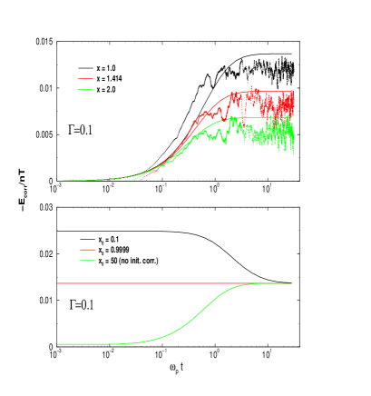
FIG. 2.: The formation of correlation energy $-{\cal E}_{\rm corr}={\rm E}_{\rm total}-{\cal E}_{\rm init}-{\cal E}_{\rm coll}={\cal E}_{\rm kin}$ in a plasma with Debye interaction $V_{i}$. The upper panel compares the analytical results (58) with MD simulations from [16] for three different ratios of $\kappa_{D}$ to the inverse Debye length $x=\kappa_{D}/\kappa$. In the lower panel we compare theoretical predictions for the inclusion of Debye initial correlations characterized by $x_{0}=\kappa_{0}/\kappa$ where $x=\kappa_{D}/\kappa=1$.

On very short time scales we can neglect the change in the distribution function. Assuming a Maxwellian initial distribution with temperature $T$ and neglecting degeneracy, we can calculate explicitly the collision integrals and obtain analytical results. We choose as a model interaction a Debye potential $V_{i}(q)=4\pi e^{2}\hbar^{2}/[q^{2}+\hbar^{2}\kappa_{i}^{2}]$ with fixed parameter $\kappa_{i}=\kappa_{D}$ and for the initial correlations $\kappa_{i}=\kappa_{0}$. We obtain for the change of kinetic energy on short times from (38) and (41)

$${\partial\over\partial t}E_{\rm kin}(t)={\cal E}[V(q)^{2}](t)-{\cal E}[V_{0}(q)V(q)](t),$$ (56)

which can be integrated [6] to yield

$$E_{\rm kin}(t)=E_{\rm total}-E_{\rm init}(t)-E_{\rm coll}(t).$$ (57)

For the classical limit we obtain explicitly the time dependent kinetic energy

$${E_{\rm coll}(t)\over nT}=-{\sqrt{3}\Gamma^{3/2}\over 4x}\partial_{y}(y{\cal F}(y))_{y=x\tau},$$ (58)

where ${\cal F}(y)=1-{\rm e}^{y^{2}}{\rm erfc}(y),$ $\tau=t\omega_{p}/\sqrt{2}$, $x=\kappa_{D}/\kappa$ and $\kappa^{2}=4\pi e^{2}n/T=\omega_{p}^{2}T/m$. The plasma parameter is given as usually by $\Gamma={e^{2}\over a_{e}T}$, where $a_{e}=({3\over 4\pi n})^{1/3}$ is the Wigner-Seitz radius.

In Fig. 2, upper panel, we compare the analytical results of (58) with MD simulations [16] using the Debye potential $V_{i}$ as bare interaction. The evolution of kinetic energy is shown for three different ratios $x$. The agreement between theory and simulations is quite satisfactory, in particular, the short time behavior for $x=2$. The stronger initial increase of kinetic energy observed in the simulations at $x=1$ may be due to the finite size of the simulation box which could more and more affect the results for increasing range of the interaction.

Now we include the initial correlations choosing the equilibrium expression (47) which leads to

$${E_{\rm init}(t)\over nT} = -{\sqrt{3}\Gamma^{3/2}\over{2(x_{0}^{2}-x^{2})}}\left[x{\cal F}(x\tau)-x_{0}{\cal F}(x_{0}\tau)\right],$$ (59)

where $x_{0}=\kappa_{0}/\kappa$ characterizing the strength of the initial Debye correlations (47) with the Debye potential $V_{0}$ which containes $\kappa_{0}$ instead of $\kappa_{D}$. Besides the kinetic energy (59) from initial correlations, the total energy $E_{\rm total}$ (57) now includes the initial correlation energy which can be calculated from the long time limit of (58) leading to

$${E_{\rm total}\over nT}={\sqrt{3}\Gamma^{3/2}\over 2(x+x_{0})}.$$ (60)

The result (57) is seen in Fig. 2, lower panel. We observe that if the initial correlation is characterized by a potential range larger than the Debye screening length, $x_{0}<1$, the initial state is over–correlated, and the correlation energy starts at a higher absolute value than without initial correlations relaxing towards the correct equilibrium value. If, instead, $x_{0}=1$ no change of correlation energy is observed, as expected. Similar trends have been observed in numerical solutions [9].

In summary, in this Letter initial correlations are investigated within kinetic theory. Explicit correction terms appear on every level of perturbation theory correcting the non-Markovian kinetic equation properly in a way that the collision integral vanishes if the evolution starts from a correlated equilibrium state. Furthermore, the conservation laws of a correlated plasma are proven including the contributions from initial correlations. It is shown that besides the appearance of correlation energy a correlated flux appears if higher than Born correlations are considered.

Deriving analytical formulas for high temperature plasmas allowed us to investigate the time dependent formation of the correlation energy and the decay of initial correlations. The comparison with molecular dynamics simulations is found to be satisfactorily. Including initial correlations the cases of over- and under-correlated initial states are discussed. While starting from equilibrium the correlation energy does not change, for over- and under-correlated states the equilibrium value is approached after a time of the order of the inverse plasma frequency.

The many interesting discussions with Pavel Lipavský, Václav Špička and D. Semkat are gratefully acknowledged. G. Zwicknagel is thanked for providing simulation data prior to publication.

REFERENCES

• [1] V. Špička, P. Lipavský, and K. Morawetz, Phys. Lett. A 240, 160 (1998).
• [2] D. Kremp, M. Bonitz, W. Kraeft, and M. Schlanges, Ann. of Phys. 258, 320 (1997).
• [3] M. Bonitz, Quantum Kinetic Theory (Teubner, Stuttgart, 1998).
• [4] I. B. Levinson, Fiz. Tverd. Tela Leningrad 6, 2113 (1965).
• [5] I. B. Levinson, Zh. Eksp. Teor. Fiz. 57, 660 (1969), [Sov. Phys.–JETP 30, 362 (1970)].
• [6] K. Morawetz, V. Špička, and P. Lipavský, Phys. Lett. A 246, 311 (1998).
• [7] D. Lee, S. Fujita, and F. Wu, Phys. Rev. A 2, 854 (1970).
• [8] P. Danielewicz, Ann. Phys. (NY) 152, 239 (1984).
• [9] D. Semkat, D. Kremp, and M. Bonitz, Phys. Rev. E 59, 1557 (1999).
• [10] V.G. Morozov, G. Röpke, Ann. Phys. (NY) submitted.
• [11] L. P. Kadanoff and G. Baym, Quantum Statistical Mechanics (Benjamin, New York, 1962).
• [12] P. Lipavský, V. Špička, and B. Velický, Phys. Rev. B 34, 6933 (1986).
• [13] D. N. Zubarev, V. Morozov, and G. Röpke, Statistical Mechanics of Nonequilibrium Processes (Akademie Verlag, Berlin, 1997), Vol. 2.
• [14] K. Morawetz, Phys. Lett. A 199, 241 (1995).
• [15] It is interesting to note that the corrections to the next Born approximation (33) due to initial correlations is of the type found in impurity scattering. Therefore the initial correlations higher than $\sim V^{2}$ are governed by another type of dynamics than the build up of correlations involved in ${\cal I}$ and ${\cal I}_{0}$.
• [16] G. Zwicknagel, Contrib. Plasma Phys. 39 (1999) 1-2,155, and private communications