Beam Test of Gamma-ray Large Area Space Telescope Components

Abstract

A beam test of GLAST (Gamma-ray Large Area Space Telescope) components was performed at the Stanford Linear Accelerator Center in October, 1997. These beam test components were simple versions of the planned flight hardware. Results on the performance of the tracker, calorimeter, and anti-coincidence charged particle veto are presented.

1 Introduction

GLAST[1] is the next high-energy gamma-ray mission, scheduled to be launched by NASA in 2005. This mission will continue and expand the exploration of the upper end of the celestial electromagnetic spectrum uncovered by the highly successful EGRET[2] experiment, which had full sensitivity up to $\approx 10$ GeV. The design of the GLAST instrument is based on that of EGRET, which is a gamma-ray pair-conversion telescope, with the primary innovation being the use of modern particle detector technologies. GLAST will cover the energy range 20 MeV-300 GeV, with capabilities up to 1 TeV. It will have more than a factor of 30 times the sensitivity of EGRET in the overlapping energy region (20 MeV - 10 GeV). With unattenuated sensitivity to higher than 300 GeV, GLAST will cover one of the most poorly measured regions of the electromagnetic spectrum. These new capabilities will open important new windows on a wide variety of science topics, including some of the most energetic phenomena in Nature: gamma-ray bursts, active galactic nuclei and supermassive black holes, the diffuse high-energy gamma-ray extra-galactic background, pulsars, and the origins of cosmic rays. GLAST will also make possible searches for galactic particle dark matter annihilations and other particle physics phenomena not currently accessible with terrestrial accelerators. In addition, GLAST will provide an important overlap in energy coverage with ground-based air shower detectors, with complementary capabilities. GLAST has been developed by an interdisciplinary collaboration of high-energy particle physicists and high-energy astrophysicists.

The pair-conversion measurement principle allows a relatively precise determination of the direction of incident photons and provides a powerful signature for the rejection of charged particle cosmic ray backgrounds, which have a flux as great as $10^{4}$ times that of cosmic gamma-ray signals. The instrument consists of three subsystems: a plastic scintillation anti-coincidence detector (ACD) to veto incident charged particles, a precision converter-tracker to record gamma conversions and to track the resulting $e^{+}e^{-}$ pairs, and a calorimeter to measure the energy in the electromagnetic shower. Particles incident through the instrument’s aperture first encounter the ACD, followed by the converter-tracker, and finally the calorimeter. The technologies selected for the subsystems are in common use in many high-energy particle physics detectors. In GLAST, the scintillation light from the ACD tiles is collected and transported by wavelength-shifting fibers to miniature photomultipliers. The tracking pair converter section (tracker) has layers of thin sheets of lead, which convert the gammas, and the co-ordinates of resulting charged tracks are measured in adjacent silicon strip detectors. The calorimeter is a 10 radiation length stack of segmented, hodoscopically-arranged CsI crystals, read out by photodiodes. While the basic principles of these components are well-understood, adapting them for use in a satellite-based instrument presents challenges particularly in the areas of power and mass. The tracker, calorimeter and associated data acquisition system are modular: the baseline instrument comprises a 5x5 array of 32x32 cm towers. In addition to simplifying the construction of the flight instrument, the modularity also allows detailed testing and characterization of all critical aspects of detector performance in the full, flight-size configuration early in the development program.

A detailed Monte Carlo simulation of GLAST was used to quantify our understanding of these technology choices and to optimize the design. To verify the results obtained by the computer analysis simple versions of all three subsystems were constructed and tested together in an electron and tagged photon beam in End Station A at SLAC. The goals of these tests for each of the subsystems included the following:

ACD

1. Check the efficiency for detecting minimum ionizing particles (MIPs) using fiber readout of scintillating tiles.

2. Investigate the backsplash from showers in the calorimeter, which causes false vetoes, as a function of energy and angle (this self-veto was the primary limitation of the sensitivity of EGRET at high energy).

Tracker

1. Demonstrate the merits of a silicon strip detector (SSD) pair conversion telescope.

2. Validate the computer modeling and optimization studies with respect to converter thickness, detector spacing and SSD pitch.

3. Validate the prototype, low power front end electronics used to read out the SSDs.

CsI Calorimeter

1. Demonstrate the hodoscopic light sharing concept for co-ordinate measurement in transversely mounted CsI logs, and validate the shower imaging performance.

2. Measure the energy resolution.

3. Study leakage corrections using longitudinal shower profile fitting at high energies.

For each of these tests, the presence of the other subsystems proved valuable: for tracker studies (particularly at low energies) the calorimeter provided the measurement of the photon energy; for calorimeter studies the tracker provided a precision telescope to locate the entry point and direction of the beam particle; and for all tests the ACD system was used to discard contaminated events (e.g., accompanying low-energy particles coming down the beam pipe). We report here the results of these studies. In section 2, the experimental setup of the beamline and the detectors is described. The performance of the individual detectors is given in section 3, followed by a compendium of results from the studies for each subsystem in section 4 and a summary in section 5.

2 Experimental setup

2.1 Beamline and Trigger

The experiment was performed in End Station A (ESA) at the Stanford Linear Accelerator Center (SLAC). A technique was recently developed[3] to produce relatively low-intensity secondary electron and positron beams parasitically from the main LINAC beamline, which delivers beams with energy up to 50 GeV at a 120 Hz repetition rate. A schematic is shown in figure 1. A small fraction of the LINAC electron beam is scraped by collimators, producing bremsstrahlung photons that continue downstream, past bending magnets, producing secondary electrons and positrons when they hit a 0.7 $X_{0}$ target. Electrons within an adjustable range of momentum (typically 1-2%) are transported to ESA. Beamline parameters were adjusted to allow an average of one electron per machine pulse into ESA.

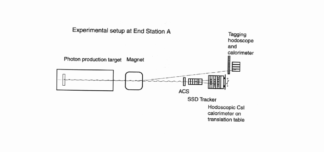
Figure 2: Schematic of the tagged photon beam.

In addition to the electron beam, a tagged photon beam was also generated, as shown in figure 2. A movable target with 2.5%, 5% and 10% $X_{0}$ copper foils produced bremsstrahlung photons from the ESA electron beam (a 25 GeV ESA electron beam was used for most of the photon runs). A large sweeping magnet ($B0$) deflected the electron beam toward an 88-channel two-dimensional scintillator hodoscope, followed by a set of four lead-glass block calorimeters.

The data acquisition system[4] collected data from every machine pulse. More than 400 data runs were taken during a four week period, resulting in $2.1\times 10^{8}$ triggers and over 200 GB of data.

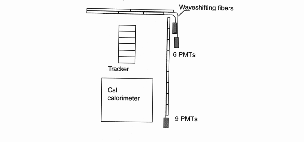
Figure 3: Schematic of the GLAST beam test detectors.

The GLAST experimental setup is shown schematically in figure 3. Each of the subsystems is described in the following sections.

2.2 ACD

Although an anticoincidence system is essential to distinguish the cosmic gamma-ray flux from the much larger charged particle cosmic ray flux seen by a gamma-ray telescope in orbit, a monolithic scintillator detector such as used by SAS-2[5], COS-B[6], and EGRET is neither practical for an instrument the size of GLAST nor desirable. The highest-energy gamma rays (especially with energies above 10 GeV) produce backsplash: low energy photons originating in the calorimeter as the products of the electromagnetic shower. Such backsplash photons can cause a veto pulse in the ACD through Compton scattering. The EGRET detector has a monolithic ACD and suffers a $\approx$50% loss of detection efficiency at 10 GeV due to this effect[7]. This self-veto can be reduced by segmenting the GLAST ACD into tiles and vetoing an event only if the pulse appears in the tile through which the reconstructed event trajectory passes. Monte Carlo simulations indicate that this approach reduces the self veto rate at 30 GeV by at least an order of magnitude.

The beam test ACD consisted of two modules, as shown in figure 3. One module contained 9 scintillating paddles (Bicron BC-408) and was placed on the side of the tracker/calorimeter. The front module consisted of two superimposed layers with 3 paddles in each and was placed just upstream of the tracker. Wave-shifting fibers (BCF-91A, 1 mm diameter), matching the BC-408 scintillator, were embedded in grooves across the 1 cm-thick paddles to collect and transfer light to Hamamatsu R647 photo-multiplier tubes. Each phototube was packaged in a soft-iron housing for magnetic field shielding and was equipped with a variable resistor to adjust the gain. The signal from each phototube was pulse-height analyzed by a CAMAC 2249A PHA module.

2.3 Tracker

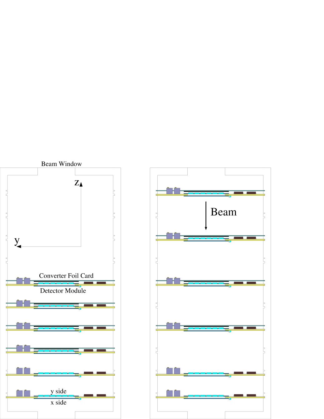
Figure 4: Layout of the beam test tracker. The “pancake” configuration is shown on the left and the “stretch” configuration on the right. Both configurations are shown with converter foil cards installed in front of the first four modules. The $x$ coordinate axis goes into the page.

The silicon-strip tracker consisted of six modules, each with two detector layers, one oriented to measure the $x$ coordinate and the other oriented to measure $y$. The detectors were single-sided AC-coupled silicon strip detectors manufactured by Hamamatsu Photonics. They were 6 cm by 6 cm in size and 500 $\mu$m thick with an $n$-type substrate and $p$-type strip implants. The strips were 57 $\mu$m in width and 236 $\mu$m in pitch, with a total capacitance of about 1.2 pF per centimeter of strip length. The strip implants were biased at about 10 V via punchthrough structures, while the back side was biased at 140 V for full depletion, except during special runs in which the bias voltage was varied in order to study the efficiency as a function of depletion depth. The detectors were mounted on the two sides of a printed-circuit card, along with the readout electronics and cable connectors. To minimize scattering of the beam, each card was cut out under the detector active area, and windows were cut out of the acrylic housing. The entire assembly was wrapped in aluminized mylar for shielding from light and electromagnetic interference. Figure 4 shows the two general configurations used in the beam test. The “pancake” configuration had a 3 cm spacing between modules, similar to the baseline GLAST design, while in the “stretch” configuration that spacing was doubled, except for the space between the last two modules. The configuration was easily changed by sliding the modules in and out of grooves machined in the housing. The lead converter foils were mounted on separate cards that could also be slid in and out of grooves located directly in front of each detector plane. In figure 4 the converter foils are shown installed in the first four modules. The gap between the lead and the first detector was about 2 mm, while the gap between the two detector sides within a module was 1.5 mm.

Each readout channel was connected to a single 6 cm long strip, except for the $y$ side of the first module encountered by the beam which had five detectors connected in series to make 30 cm long strips. Only that module was used for studies of the noise performance, since only it had input capacitance close to that of the GLAST baseline design.

Consecutive strips were instrumented in each detector with six 32-channel CMOS chips that were custom designed to match the detector pitch and satisfy the GLAST power and noise requirements. Due to limitations on the number of available readout chips, only 192 of the total 256 strips on each detector were instrumented with readout electronics. Each channel consisted of a charge-sensitive preamplifier, a shaping amplifier with approximately 1 $\mu$s peaking time, a comparator, a programmable digital mask, and a latch. In addition, the six chips in each readout section provided a 192-wide logical OR of the comparator outputs (after the mask) to provide the self-triggering capability required for GLAST. In the beam test, however, the system was triggered by the beam timing. About 1 $\mu$s after the beam passed through the apparatus the latches were triggered, after which the 192 bits were shifted serially out of each readout section. In addition, the start-time and length of the logical-OR signals were digitized by TDC’s to study the self-triggering capability offline.

The custom readout electronics operated with a power consumption of 140 $\mu$W per channel and an rms equivalent noise charge of 1400 electrons (0.22 fC) for the 30-cm long strips. Except for runs in which it was varied to study efficiency, the threshold was generally set at about 1.5 fC, compared with the more than 6 fC of charge deposited by a single minimum ionizing particle at normal incidence. The typical rms variation of the threshold across a 32-channel chip was under 0.12 fC. The tracker readout electronics are described in more detail in reference [8].

2.4 CsI calorimeters

The calorimeter comprised eight layers of six CsI(Tl) crystals read out by PIN photodiodes. Each layer was rotated $90^{\circ}$ with respect to its neighboring layers, forming an x-y hodoscopic array. The crystal blocks were $3\times 3\times 19$ cm in size and individually wrapped in Tetratek and aluminized mylar. Hamamatsu S3590 PIN photodiodes, with approximately 1 cm² active area, were mounted on each end to measure the scintillation light from an energy deposition in the crystal. The difference in light levels seen at the two ends provided a determination of the position of the energy deposition along the crystal block.

Although 48 crystals would be required to form the complete calorimeter, only 32 CsI(Tl) crystals were available for the test. Brass supporting blocks were therefore used to fill the remaining 16 positions to complete the hodoscopic array. Figure 5 shows the general arrangement of the calorimeter and the positions of the passive blocks. In the figure, the brass blocks are shaded and the CsI blocks are light with PIN photodiodes indicated on the ends. The arrangement of the active CsI blocks was designed to study events normally incident near the front center of the calorimeter. Off-axis response could be studied by directing the beam from the front center toward the lower right corner in the figure where the calorimeter was fully populated with active CsI blocks.

The crystal array was mounted in an aluminum frame consisting of four walls with PIN photodiode access holes and a bottom structural plate. In figure 5, two of the walls have been removed. The frame was open on the front where the beam entered the calorimeter. The calorimeter was enclosed in a light-tight aluminum shield and mounted on a precision translation table which permitted both vertical and horizontal adjustment of the beam position on the front of the calorimeter. This translation table was used to study the position resolution by mapping the relative light levels over the entire length of the CsI blocks. In these tests the tracker remained fixed and provided accurate beam positions, while the calorimeter was moved relative to the beam and tracker to map the entire crystal array.

The PIN diodes were biased by 35 volt batteries and attached to eV Products 5092 hybrid preamps. The preamps were mounted on circuit cards adjacent to the PIN diodes. The outputs of the 64 preamps were routed to a CAMAC/NIM data acquisition system consisting of CAEN shaping amplifiers and Phillips or LeCroy 12 bit analog to digital converters. The CAEN shaping amplifiers provided programmable gain adjustments to optimize the electronics for the specific beam energies of each test.

2.5 Online data spying, event display, and offline filtering

The online system sampled events from the data stream and made simple data selections in real time. This enabled us to monitor the performance of the individual detectors and to tune various beam parameters while collecting data. The online monitoring system included a single event display with rudimentary track reconstruction and full online histogramming capabilities.

Offline processing reduced the volume of data for storage and distribution. Most of the beam pulses did not result in photon events, due to the thin target radiators we used. To separate real events from empty pulses we applied very loose selection criteria on the raw data, requiring either hits in three consecutive x-y tracker planes or at least 6 MeV of energy deposited in the calorimeter. Event filtering removed approximately 80% of the raw data in photon mode and approximately 30% in electron mode.

3 Detector performance

3.1 ACD

The overall response and efficiency of the ACD were investigated using a 25 GeV electron beam. Typical pulse height histograms are shown in figure 6 for (a) a tile that was crossed by a direct electron beam, and (b) a tile outside the direct beam. The peak corresponding to one MIP is clearly seen in (a), near channel 100. The backsplash spectrum appears in low channels of histogram (b).

The efficiency was determined using a sample of electron beam events that had hits in all 12 tracker planes within 1 cm of the beam axis by counting the fraction of these events that had a coincident hit in the relevant ACD tile. For thresholds below 0.35 MIP, the inefficiencies were always smaller than $5\times 10^{-4}$.

3.2 Tracker

The efficiency to detect minimum-ionizing particles and the occupancy due to random noise were measured. The efficiency must be close to 100%: to realize the optimal angular resolution of the device it is crucial not to miss either of the first two $xy$ pairs of measurements on a track. The noise occupancy must be low, not only to avoid flooding the data stream but, more importantly, to avoid saturating the readout system with spurious triggers. In GLAST, the tracker will be employed in the first-level trigger, which simply looks for a coincidence among three consecutive $xy$ pairs of silicon layers. The rate for this trigger depends very strongly on the occupancy: with a 1 $\mu$s coincidence window the single-channel noise occupancy must be less than $10^{-4}$ so that spurious triggers do not dominate the overall trigger rate. A major objective of the beam test was to demonstrate that such a low occupancy can be achieved with the prototype electronics without degrading the detection efficiency.

3.2.1 Tracker noise occupancy

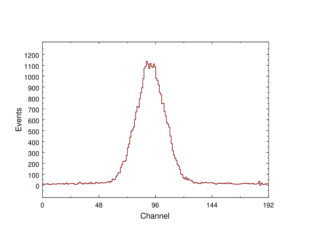
Figure 7: The beam profile as measured in the $y$ coordinate by tracker module 4. The strip pitch is 236 $\mu$m.

Only the first layer of detectors struck by the beam had five detectors ganged in series, so it was the only relevant testbed for studies of the noise occupancy. (Due to poor quality control at the wire bonding vendor, a number of detector strips in the five-detector module were damaged in random locations. These were known prior to the beam test and have been removed from the analysis.) The other single-detector modules had low capacitance and therefore almost unobservably low noise, with the exception of very few damaged strips. The efficiency, however, is not expected to depend significantly on the capacitance, so it could be studied with the single detector modules as well as the first five-detector layer. Figure 7 shows the vertical beam profile. It is well contained within the 4.5 cm instrumented region of the detector.

In the case that random hits are due to electronic noise, the dependence of the threshold-crossing rate, or noise rate, on the threshold level $V_{t}$ is well approximated by [9]

$$f_{n}=f_{0}\cdot e^{-V_{t}^{2}/2\sigma_{n}^{2}}\,,$$ (1)

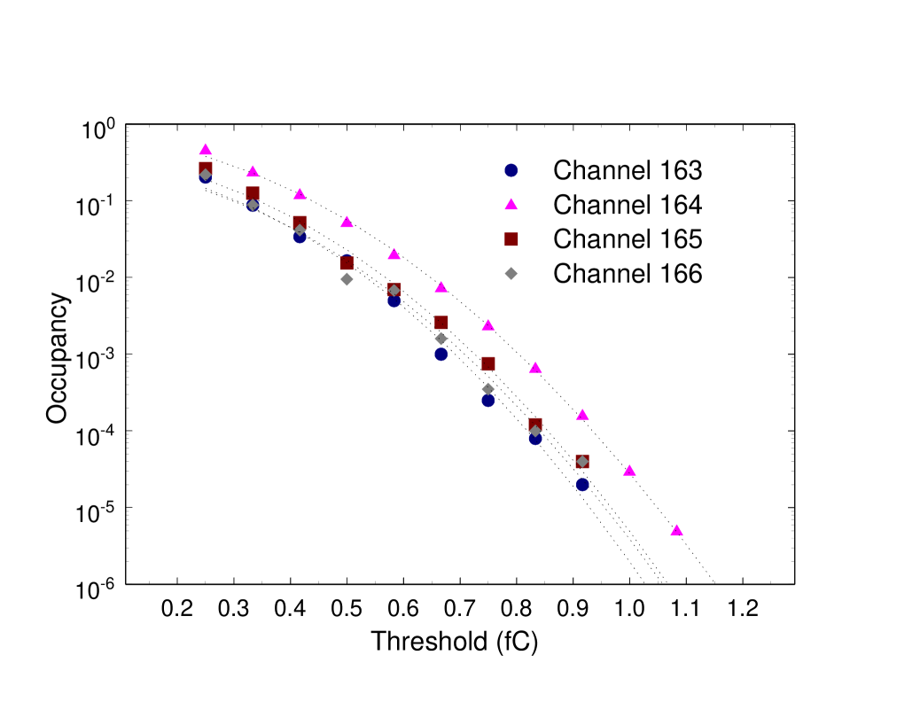
Figure 8: The noise occupancy versus threshold in four channels near the center of the beam profile in the five-detector module. The threshold is given in terms of equivalent noise charge at the preamplifier input. One fC represents a voltage at the discriminator input of about 115 mV. The smooth curves are fits to the equation in the text. From the fits, the rms noise values of channels 163 through 166 are 1277, 1386, 1315, and 1322 electrons respectively.

where $\sigma_{n}$ is the rms noise level at the discriminator input. Figure 8 shows the occupancy for four typical channels of the five detector module. For these measurements all channels but one were masked off at the output of the comparator. The rms noise is extracted by fitting the curves to Eqn. 1, with the results plotted as smooth dotted curves in figure 8. The value of $\sigma_{n}$ in those four fits ranges from 1290 electrons to 1390 electrons (0.21 fC to 0.22 fC) equivalent noise charge referenced to the preamplifier input. The channel-to-channel variation in noise occupancy is primarily due to threshold variations. The typical rms variation across a 32-channel chip was 0.05 fC, with a few chips showing rms variations as large as 0.14 fC.

The occupancy increased significantly, however, when the outputs of all channels were enabled. In that condition the logical-OR of all channels (Fast-OR) —which is to be used for triggering— runs much faster, and its signal was observed to feed back to the amplifiers, causing a shift in the effective threshold. Steps have been taken to solve this problem by improving the grounding and and power-supply isolation and decoupling of the circuit board onto which the chips are mounted; by changing the CMOS Fast-OR outputs to low-voltage differential signals; and by decreasing the digital power supply from 5 V to 3 V. A prototype chip and circuit board fabricated with these new features does not exhibit this feedback problem—the occupancy no longer depends on the number of enabled channels.

3.2.2 Tracker efficiency

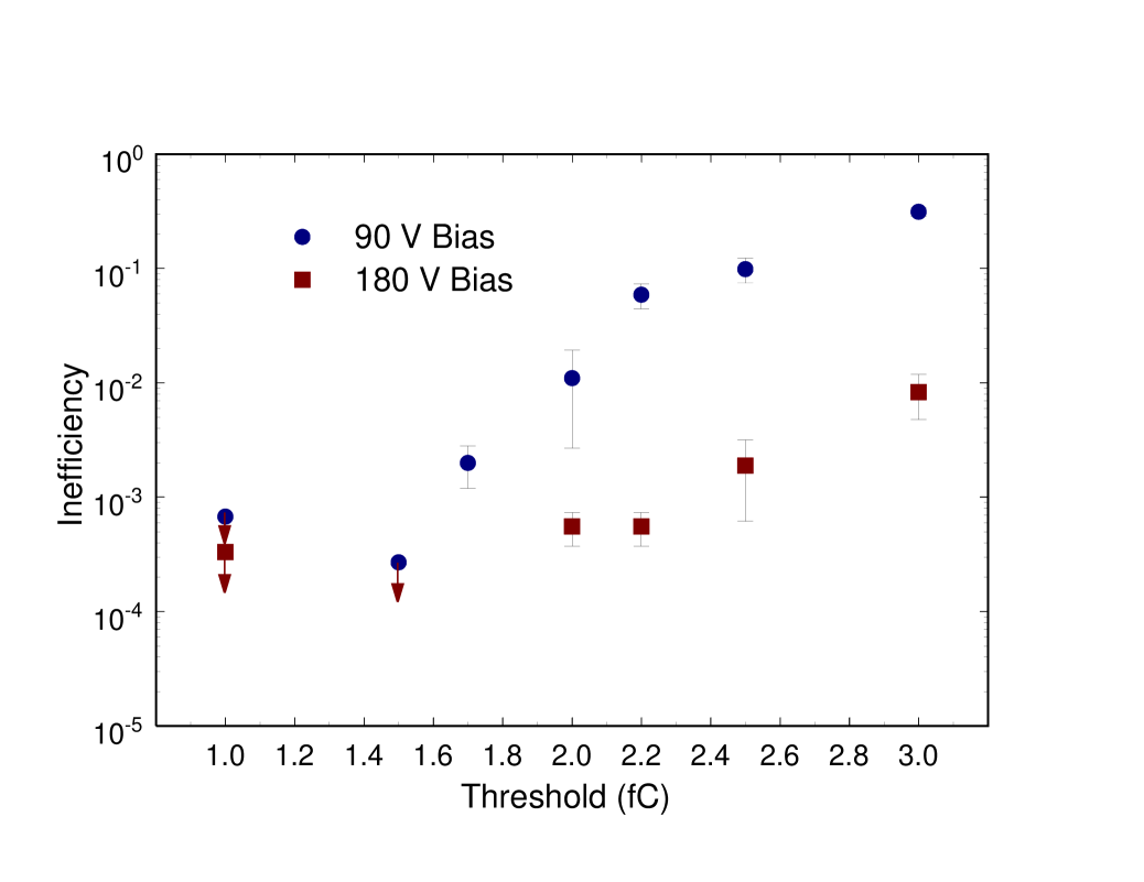
Figure 9: The measured tracker single-plane inefficiency versus threshold setting for two different bias voltages. The measurements were made using events with single 25 GeV electrons.

The efficiency was measured for the five-detector module and a single-detector module. The remaining four modules were used as anchor planes to reconstruct the track. A 25 GeV electron beam was used. Single particle events were selected by requiring that the calorimeter signal was consistent with a single-electron shower and that only one track was reconstructed in the tracker. For the detectors under test, a hit was counted if it was found within 4 strips of the position predicted from the track. The bias voltage was varied to change the depletion thickness and, therefore, the amount of ionization deposited. At about 180 V the 500 $\mu$m detectors were fully depleted. A 90 V bias voltage yielded a depletion thickness between 360 $\mu$m and 390 $\mu$m, close to the envisaged GLAST detector thickness of 400 $\mu$m. Figure 9 shows the inefficiency versus threshold setting for the two bias voltages. The upper limits reflect the limited number of recorded events (about $10^{4}$). No significant difference in efficiency was observed between the single-detector planes and the five-detector plane.

From figures 8 and 9 it is evident that the tracker can be operated at essentially 100% efficiency with an occupancy well below $10^{-4}$ by setting a threshold in the range of 1-1.5 fC. The GLAST signal-to-noise and trigger requirements have been met and exceeded, while the 140 $\mu$W per channel consumed by the amplifiers and discriminators satisfies the GLAST power restrictions. More recent tests with prototype chips containing the full GLAST digital readout capability have demonstrated that, even with the digital activity included, the per-channel power can meet the goal of 200 $\mu$W.

3.2.3 Fast-OR

The Fast-OR signal was studied in the beam test using multi-hit TDC’s. The distribution of the time of the leading edge is important for understanding the GLAST trigger timing requirements. It was measured with high-energy electrons for a variety of detector bias voltages corresponding to depletion depths ranging between 200 $\mu$m and 500 $\mu$m. For full depletion, the full width of the peak at half maximum was only 50 ns. The lower bias voltages resulted in larger time fluctuations, but overall the data indicated that a trigger coincidence window of 0.5 $\mu$s could be used for minimum ionizing particles with essentially 100% efficiency.

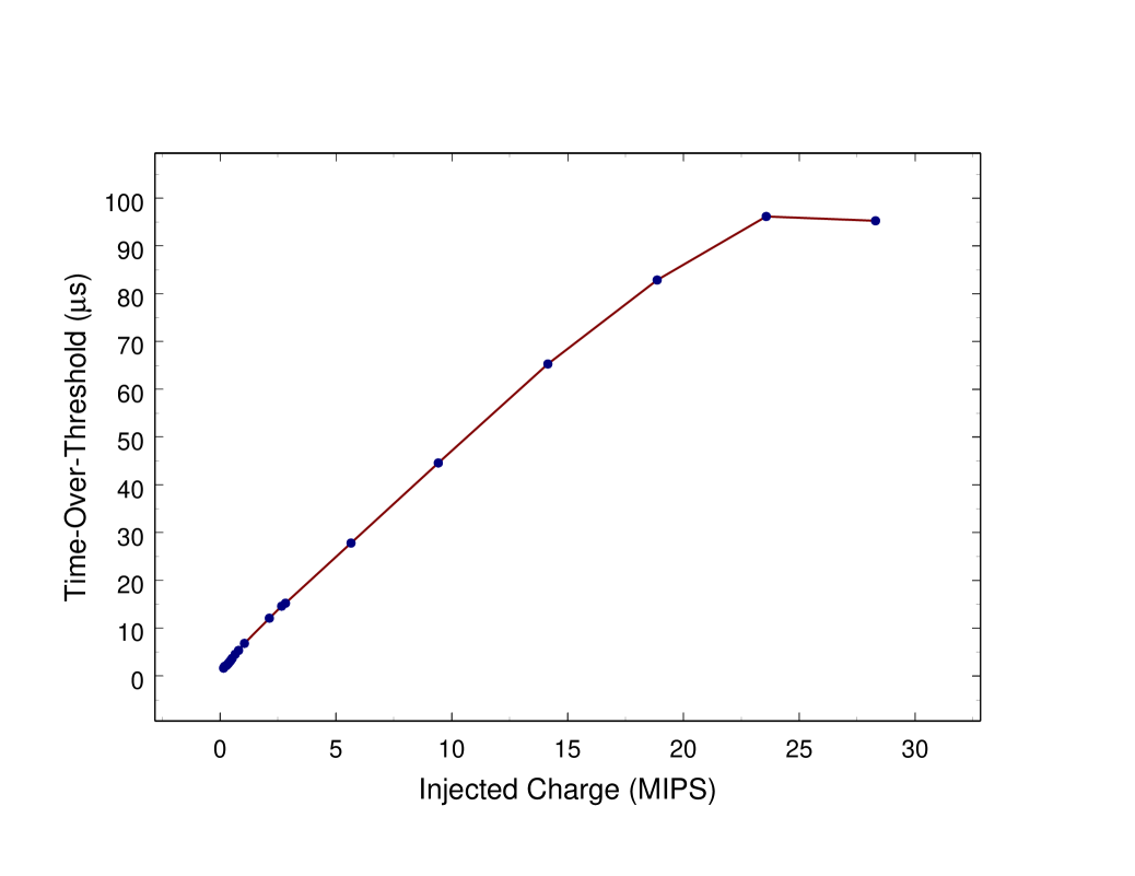
Figure 10: The time-over-threshold of the Fast-OR signal as a function of input charge injected via the internal calibration capacitors.

The GLAST experiment will record the time-over-threshold of the Fast-OR from each detector layer, along with the hit pattern. The time-over-threshold gives a rough measurement of the charge deposited by the most highly ionizing track that passed through the layer. That information can be useful for background rejection as well as for possible cosmic ray studies. Figure 10 shows the measured time-over-threshold versus input signal, obtained via charge injection, since the beam test did not provide a controlled, wide range of charge deposition. The relationship, which would be logarithmic for a true RC/CR filter, is actually fairly linear in the range 0.5-25 MIPs, where it saturates at 95 $\mu$s. This is because, for large amplitudes, the shaping amplifier reset rate is limited by a constant current source.

3.3 Calorimeter

The number of electrons produced in the photodiodes per MeV deposited energy was measured in several channels of the CsI calorimeter array. To calibrate the yield, a known charge was injected into each channel and the response was compared with the pulse height distribution produced by cosmic-ray muons, which typically deposit $\simeq$20 MeV in a crystal. The yield was typically $\sim$12,000-15,000 electrons per MeV per photodiode in the 19-cm CsI bars with a 3 $\mu$s amplifier shaping time.

4 Studies

4.1 ACD studies

The nine scintillator tiles on the side of the tracker/calorimeter and those on the top that were not directly illuminated by the beam were used to measure the backsplash. Figure 11 shows, as a function of threshold, the fraction of events that were accompanied by a pulse in tile number 9 which, when viewed from the center of the shower in the calorimeter, was approximately 90^∘ from the direction of the incident photon. The self-veto effect is a sensitive function of this threshold. In figure 12, the fraction of events that were accompanied by an ACD pulse of greater than 0.2 MIP is shown as a function of angle with respect to the incident photon direction. To present the result in a manner that is insensitive to geometry, the vertical axis is normalized by the solid angle each tile presents when viewed from the center of the shower in the calorimeter. Only the statistical errors are displayed; the systematic errors, which may be substantial, are being evaluated. The increase at 180^∘ may be due to secondary particles in the beam accompanying the photon. Aside from this feature, and the effects of shower leakage, the backsplash is apparently approximately isotropic.

4.2 Tracker studies

4.2.1 Track reconstruction

The incident $\gamma$-ray direction is determined from the electron and positron tracks, which are reconstructed from the set of hit strips. In addition to effects of noise hits, missing hits, and spurious or ambiguous tracks, the pointing resolution is ultimately limited by hit position measurement error and by energy-dependent multiple scattering. Furthermore, the $x$ and $y$ projections of the instrument are read out separately so that, given a track in the $x$ projection, the question of which $y$ track corresponds to it is ambiguous. Clearly, a good method of finding and fitting electron tracks will be critical for GLAST.

The Kalman filter [10] is an optimal linear method for fitting particle tracks. A practical implementation has been developed by Frühwirth[11]. The problem simplifies in the limit where either one of the resolution-limiting effects is negligible: if the measurement error were negligible compared to effects of multiple scattering, as expected at low energies, the filter would simply “connect the dots,” making a track from one hit to the next; however, if the measurement error were completely dominant and multiple scattering effects were negligible (e.g., at high energy), all hits would have information and one would essentially fit a straight line to the hits. The Kalman filter effectively balances these limits.

The basic algorithm we have adopted is based on the Frühwirth implementation. At each plane the Kalman filter predicts, based on the information from the prior planes, the most likely location of the hit for a projected track. Usually, the hit nearest to that predicted location is then assumed to belong to the track. This simple approach is complicated by opportunities for tracks to leave the tracker or to share a hit with another track. For each event, the algorithm looks for electron tracks in the two instrument projection planes ($xz$ and $yz$) independently. The fitted tracks are used to calculate the incident photon direction, as described in the following sections.

4.2.2 Simulations

Simulations of the beam test instrument were made using a version of glastsim [12] specially modified to represent the beam test instrument. glastsim is the code used to simulate the response of the entire GLAST instrument via the detailed interactions of particles with the various instrument and detector components [1]. The Monte Carlo code was modified for the beam test application to include the $e^{-}$ beam, the Cu conversion foil, and the magnet used for analyzing the tagged photon beam, as well as the beam test instrument. Simulated data were analyzed in the same way as the beam test data.

4.2.3 Cuts on the Data

Each event used in the analysis was required to pass several cuts. First, the Pb glass blocks used for tagging must have indicated that there was only one electron in the bunch. This lowered the probability of having multiple $\gamma$-rays produced at the bremsstrahlung target. Second, the Anti-Coincidence tiles through which the $\gamma$-ray beam passed were each required to have less than $1/4$ MIP of energy registered. This ensured that the $\gamma$-ray did not convert inside the ACD tile and that the event was relatively clean of accompanying low-energy particles from the beamline. Depending on run conditions, this left about 30% of the data for further analysis. Three more cuts were imposed based on the parameters of the reconstructed tracks: tracks must have had at least three hits regardless of the energy in the calorimeter, a reduced $\chi^{2}<5$, and the starting position of the track must have been at least $4.7$ mm from the edge of the tracker. This last requirement lowered the probability that a track might escape the tracker, which could bias the reconstructed track directions. These overall track definition cuts further reduced the data by about one third.

In an effort to make the beam test data as directly comparable with Monte Carlo simulations as possible, the Monte Carlo data were subjected to very similar cuts. The Monte Carlo included an anti-coincidence system, and a similar cut was made to reject events which converted in the plastic scintillator. All of the cuts based on track parameters were made in the same way for both the Monte Carlo and the beam test data.

4.2.4 Reconstructing photon directions

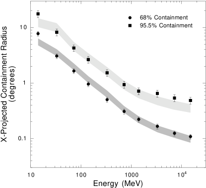
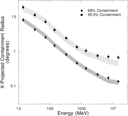
Figure 13: X-Projected angular resolutions for the pancake configuration with no Pb radiators (left) and 4% Pb radiators (right). Circles indicate the 68% containment width, and squares indicate the 95.5% containment width. Error bars are 2$\sigma$ statistical errors, and shaded regions represent the 2$\sigma$ confidence regions of the Monte Carlo estimates.

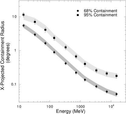
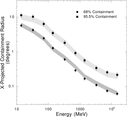
Figure 14: X-Projected angular resolutions for the stretch configuration with no Pb radiators (left) and 4% radiators (right). Circles indicate the 68% containment width, and squares indicate the 95.5% containment width. Error bars are 2$\sigma$ statistical errors, and shaded regions represent the 2$\sigma$ confidence regions of the Monte Carlo estimates.

Since the average pair conversion results in unequal sharing of the $\gamma$-ray energy, and since multiple scattering effects are inversely proportional to the energy of the particle producing the track, the incident $\gamma$-ray angles were calculated using a weighted average of the two track directions, with the straighter track receiving 3/4 of the total weight. The projected instrument angular resolution could be measured by examining the distribution of reconstructed incident angles. As this distribution had broader tails than a Gaussian, the 68% and 95% containment radii were used to characterize it. For each instrument configuration, these parameters were measured as a function of energy in ten bands. The same reconstruction code was used to analyze the Monte Carlo simulations, and the distribution widths were compared (figures 13 and 14). The simulated distributions show good agreement with the data out to the 95% containment radius and beyond.

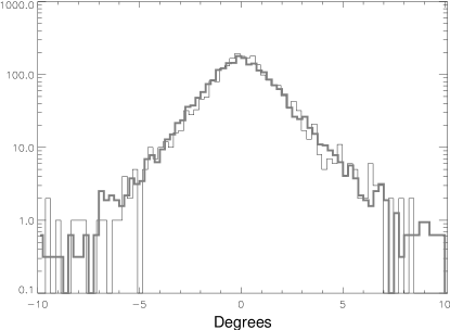
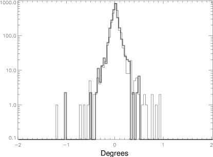
Figure 15: Reconstructed $\gamma$-ray angle distributions for beam test and Monte Carlo data for pancake 4% $X_{0}$ (left) and stretch with no Pb radiators (right). Thin lines are the beam test distributions, thick lines are the normalized Monte Carlo distribution.

The containment radii in each projection fall off with increasing energy somewhat faster than the $1/E$ dependence expected purely from multiple scattering, for a number of reasons. The containment radii at low energies are smaller than might be expected because of self-collimation: the finite width of the detector prevents events from being reconstructed with large incident angles. At higher energies, measurement error becomes a significant contributor to the angular resolution. While these effects cause deviations from theoretical estimates of the pointing resolution, they are well-represented by Monte Carlo simulations (see figure 15). Details of the angular resolution determination, including specifics of the track-finding algorithm, methods of dealing with noisy strips, alignment of the instrument planes, and possible systematic biases are discussed elsewhere [13].

4.3 Calorimeter studies

4.3.1 Energy reconstruction

The principal function of the calorimeter is to measure the energy of incident $\gamma$-rays. At the lower end of the sensitive range of GLAST, where electromagnetic showers are fully contained within the calorimeter, the best measurement of the incident gamma-ray energy is obtained from the simple sum of all the signals from the CsI crystals. At energies above $\sim$1 GeV, an appreciable fraction of the shower escapes out the back of the calorimeter, and this fraction increases with $\gamma$-ray energy. At moderate energies ($\sim$ few GeV), fluctuations in the shower development thus create a substantial tail to lower energy depositions; at higher energies these fluctuations completely dominate the resolution and the response distribution is again symmetric, but broader.

Figure 16 shows the distributions of energy deposition for 25 GeV electron showers in each of the 8 layers of the beam test calorimeter. A pair of distributions is shown for each layer: the left member of the pair is from the beam test data, with one event producing one point in each layer; the right member of the pair is the same distribution from the Monte Carlo simulation. The centroid and width of the beam test and Monte Carlo distributions in each layer are in good agreement quantitatively (with the exception of layers 7 and 8, where a configuration error in the ADCs blurred the distributions). The broad energy distributions seen in the figure are dominated by shower fluctuations, and the energy depositions are strongly correlated from layer to layer. Using a monoenergetic 160 MeV/nulceon ${}^{12}C$ beam at the National Superconducting Cyclotron Laboratory at Michigan State University, the intrinsic energy resolution of these CsI crystals with PIN readout was measured to be 0.3% (rms) at $\approx$ 2 GeV.

Using the longitudinal shower profile provided by the segmentation of the CsI calorimeter, one can improve the measurement of the incident electron energy by fitting the profile of the captured energy to an analytical description of the energy-dependent mean longitudinal profile. This shower profile is reasonably well-described by a gamma distribution[14] which is a function only of the location of the shower starting point and the incident energy $E_{0}$:

$$\frac{1}{E_{0}}\frac{dE}{d\xi}=\\ \frac{b(b\xi)^{a-1}\mbox{e}^{-b\xi}}{\Gamma(a)}$$ (2)

The parameter $\xi$ is the depth into the shower normalized to radiation lengths, $\xi=x/X_{0}$. The parameter $b$ scales the shower length and depends weakly on electron energy and the $Z$ of the target material; however, a good approximation is simply to set $b=0.5$. The parameter $a$ is energy-dependent with the form $a=1+b(\ln(E_{0}/E_{c})-0.5)$. $E_{c}$ is the critical energy where bremsstrahlung energy loss rate is equal to the ionization loss rate ($E_{c}\sim 14$ MeV in CsI).

The free parameters in the fit were the starting position of the shower relative to the edge of the first layer of the calorimeter and the initial electon energy, $E_{0}$. In the fitting, the shower profile of Eqn. 2 was integrated over the path length in each of the layers. The fitting permitted both early and late starts to the shower. The results of the fitting are shown in Figure 17. Panel (a) of the figure shows the histograms of the measured energy loss in the calorimeter for electron beams of 2, 25, and 40 GeV. The tails to low energy are clearly evident for the beam energies of 25 and 40 GeV. Figure 17b shows the results of the fitting as histograms of the fitted energy for 25 and 40 GeV runs. Fitting was not performed for the 2 GeV run and the slight tailing to low energy is still evident. The resolutions, $\sigma_{E}/E$, as seen in panel (b) are 4, 7 and 7% for these three energies.

4.3.2 Position reconstruction and imaging calorimetry

The segmentation of the CsI calorimeter allows spatial imaging of the shower and accurate reconstruction of the incident photon direction. Each CsI crystal provides three spatial coordinates for the energy de posited in it, two coordinates from the physical location of the bar in the array and one coordinate along the length of the bar, reconstructed from the difference in the light level measured in the photodiode at each end ($Left$ and $Right$). To reconstruct this longitudinal position, we calculate a measure of the light asymmetry, $A=(Left-Right)/(Left+Right)$, that is independent of the total energy deposited in the crystal. We note that if the light attenuation in the crystal is strictly exponential, the longitudinal position is proportional to the inverse hyperbolic tangent of the light asymmetry, $x=K\tanh^{-1}A$.

Figure 18 demonstrates that this relationship does indeed hold in the 32-cm CsI bar, and simple analytic forms can be used to convert light asymmetry to position. Positions were determined by the Si tracker for 2 GeV electrons, which typically deposited $\sim$150 MeV in this crystal. The rms error in the position, determined from light asymmetry, is 0.28 cm.

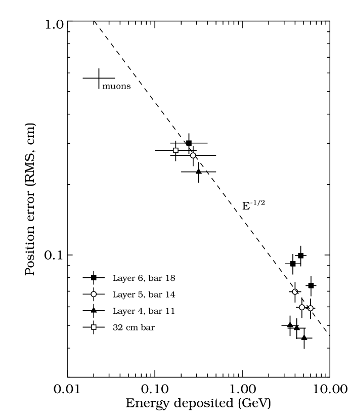
Figure 19: Position resolution, in cm, along the CsI bars for electromagnetic showers and cosmic ray muons as a function of deposited energy.

The measured rms position error is summarized in the following two figures. Figure 19 shows the position error from three crystals at increasing depth in the eight-layer CsI array at four beam energies: 2, 25, 30, and 40 GeV. The dashed line indicates that the error scales roughly as $1/\sqrt{E}$, indicating that the measurement error is dominated by photon statistics. Also shown is the position error deduced from imaging cosmic-ray muons in the array, along with that from a 2 GeV electron run in a 32-cm CsI bar identically instrumented. The muon point falls below those from electron showers because ionization energy-loss tracks do not have the significant transverse spread that EM showers have (the Moliere radius for CsI is 3.8 cm).

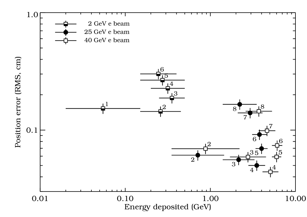
Figure 20: Energy and depth dependence of the position resolution in the calorimeter. Ordinal numbers indicate the layer in the CsI stack. The resolution degrades significantly after shower maximum.

The effect of transverse shower development on position determination can be seen in figure 20. The rms position error is shown as a function of energy deposited and depth in the calorimeter (indicated by the ordinal layer numbers on the data points) for three beam energies. We see that the position resolution is best early in the shower, where the radiating particles are few in number and tightly clustered, and at shower maximum, where the energy deposited is greatest and statistically easiest to centroid. The position resolution degrades past shower maximum, where the shower multiplicity falls and the energy deposition is spread over a larger area with variations from shower to shower.

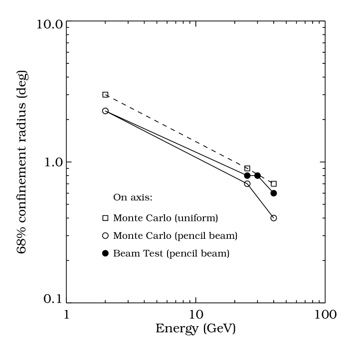
Figure 21: Measured angular resolution using only calorimeter information, as described in the text, compared with the Monte Carlo simulation.

To test the ability of the hodoscopic calorimeter to image showers, we reconstructed the arrival direction of the normally-incident beam electrons from the measured positions of the shower centroids in each layer, without reference to the tracker information. The angular resolution, given by the 68% confinement space angle, is shown by the filled circles in figure 21. The open circles indicate the angular resolution derived from a Monte Carlo simulation of a pencil beam normally incident and centered on a 3-cm $\times$ 3-cm crossing of crystals. The slightly poorer measured resolution is presumably due to systematic errors in the mapping of light asymmetry to position. Also indicated, in open squares, is the angular resolution expected from a uniform illumination at normal incidence. Here the angular resolution is degraded because of transverse sharing of the shower within crystals in a layer of the array.

5 Summary and Conclusion

The basic detector elements for GLAST were assembled and tested together for the first time in an electron and tagged photon beam at SLAC. The performance of each detector subsystem has been evaluated, and the concept of a silicon strip pair conversion telescope has been validated. The critical tracker performance characteristics (efficiency, occupancy, and power) have been investigated in detail with flight-size ladders and meet the requirements necessary for the flight instrument. Most importantly, comparison of the results with Monte Carlo simulations confirmed that the same detailed software tools that were used to design and optimize the full GLAST instrument accurately represent the beam test instrument performance. A follow-up beam test of a full GLAST prototype tower is planned for late 1999.

6 Acknowledgments

We thank the SLAC machine group and SLAC directorate for their strong support of this experiment.

7 Figures

Figure 1: Schematic layout of the SLAC ESA beamline.

Figure 5: Layout of the beam test calorimeter, as described in the text.

Figure 6: Typical ACD pulse height spectra for (a) a tile that was crossed by a direct electron beam, and (b) a tile outside the direct beam. The peak corresponding to one MIP is clearly seen in (a), near channel 100. The backsplash spectrum appears in the low channels of histogram (b).

Figure 11: Fraction of events with a backsplash pulse in tile 9, approximately 90^∘ from the incident photon direction, as a function of threshold for 5-10 and 20-25 GeV photons.

Figure 12: The fraction of events accompanied by an ACD pulse of greater than 0.2 MIPs as a function of angle with respect to the incident photon direction. The number accompanying each point indicates the ACD tile number. The vertical axis is normalized by the solid angle each tile presents when viewed from the center of the shower in the calorimeter. Errors are statistical only.

Figure 16: Energy loss distributions for each of 8 layers in the calorimeter. There are two distributions shown per layer: the distribution to the left of the layer number is from beam test events; the distribution to the right is from Monte Carlo simulations. The widths of the distributions along the abscissa are arbitrary and serve only to spread the distribution of energies for display.

Figure 17: Calorimeter response to 2, 25, and 40 GeV electrons. Panel (a) displays the total energy captured in the calorimeter. Panel (b) shows the results of longitudinal shower fitting for the 25 and 40 GeV runs as described in the text.

Figure 18: Correlation between the light asymmetry, $A=(Left-Right)/(Left+Right)$, and the incident 2 GeV electron beam position along the 32-cm CsI bar, as described in the text.

References

-
[1]
W.B. Atwood et al., Nucl.Instr.Meth. A342(1994)302;
P.F. Michelson, GLAST, a detector for high-energy gamma rays, Proc.SPIE Vol.2806, Ramsey and Parnell eds.(1996)31;
GLAST Collaboration, Proposal for the Gamma-ray Large Area Space Telescope, E.D. Bloom, G. Godfrey, and S. Ritz, ed., SLAC-R-522, 1998. - [2] E.B. Hughes et al., IEEE Trans.Nucl.Sci.,NS-27(1980)364.
- [3] M. Cavalli-Sforza et al., A method for obtaining parasitic or beams during SLAC Linear Collider Operation, SLAC-PUB-5891, 1992.
- [4] P.L. Anthony and Z.M. Szalata, Flexible high performance VME based data acquisition system for the ESA physics program, SLAC-PUB-7201, 1996.
- [5] C.E. Fichtel et al., Ap.J.198(1975)163.
- [6] G.F. Bignami et al., Space Sci.Instr. 1(1975)245.
- [7] D.J. Thompson et al., Ap.J.86(1993)629.
- [8] R.P. Johnson et al., An Amplifier-Discriminator Chip for the GLAST Silicon-Strip Tracker, to be published in IEEE Trans. Nucl. Sci., 1997 NSS/MIC conference issue, SCIPP 97-33.
- [9] S.O. Rice, Bell System Technical Journal, 23 (1944) 282 and 24 (1945) 46–156.
- [10] R.E. Kalman, Transaction of the ASME—Journal of Basic Engineering, p. 35, March 1960.
- [11] R. Frühwirth, Nucl.Instr.Meth.A262(1987)444.
- [12] T. Burnett et al., Simulating the GLAST Satellite with Gismo, submitted to Computers in Physics, 1998.
-
[13]
B.B. Jones, A Search for Gamma-Ray Bursts and Pulsars, and
the Application
of Kalman Filters to Gamma-Ray Reconstruction, Stanford University Thesis, Oct. 1998.
W.F. Tompkins, Applications of Likelihood Analysis in Gamma-Ray Astrophysics, Stanford University Thesis, March 1999. - [14] Longo, E. & Sestili, I., 1975, Nucl. Instr. and Meth. 128, 283.