Dynamics of lattice spins as a model of arrhythmia

Abstract

We consider evolution of initial disturbances in spatially extended systems with autonomous rhythmic activity, such as the heart. We consider the case when the activity is stable with respect to very smooth (changing little across the medium) disturbances and construct lattice models for description of not-so-smooth disturbances, in particular, topological defects; these models are modifications of the diffusive $XY$ model. We find that when the activity on each lattice site is very rigid in maintaining its form, the topological defects—vortices or spirals—nucleate a transition to a disordered, turbulent state.

I Introduction

Physical mechanisms underlying many cardiac arrhythmias, in particular the transition from ventricular tachycardia (VT) to ventricular fibrillation (VF), are not fully understood. The ventricular tissue is known, both experimentally and theoretically, to support long-living spiral excitations, and it is thought that a breakup of such a spiral could give rise to a turbulent, chaotic activity commonly associated with VF. (Spirals are reviewed in books [1].) A considerable effort is now being directed towards understanding of these defect-mediated transitions to turbulence within mathematical models of ventricular tissue. The currently popular approach (reviewed in Ref. [2]) considers a spiral in a patch (or slab) of ventricular tissue; the patch is taken in isolation from any pacemaking source. One then follows numerically the time evolution of that initial spiral.

In the real beating heart, however, the ventricles are not isolated from other regions, and the heart, viewed as a whole, supports a (more or less) periodic autonomous activity—the heartbeat itself. In this case, any defect should be properly viewed as a disturbance of the normal heartbeat, rather than a structure in isolated tissue. In this paper we present some general results on the evolution of initial disturbances in autonomously active media and discuss their possible applications to cardiac arrhythmias. In particular, we identify a simple mechanism of defect-induced transition to turbulence in discrete (lattice) systems. We also find that the more rigid is the system in maintaining locally the undisturbed form of activity, the more easily the transition to turbulence occurs. This observation can potentially identify a useful therapeutic target.

The assumed lattice structure need not (though it may) be related to the mechanical structure of the medium. The size of the lattice spacing in our models simply represents the smallest spatial scale on which the rhythmic activity can be desynchronized: a region smaller than that scale will necessarily fire as one. Discrete models of fibrillation have a long history, cf. the 1964 model of Moe et al. [3]. (Unlike these authors, though, we do not introduce any frozen inhomogeneity in the parameters of the medium, apart from the lattice structure itself.) In addition, the importance of a discrete (granular) structure of the medium has been emphasized in theoretical studies of defibrillation [4].

We introduce an interaction of an excitable region (like the ventricles) with a pacemaking region using the following simplified (not anatomical) model. We consider a three-dimensional (3d) slab of simulated medium whose extent in the $z$ direction is limited by the planes $z=0$ and $z=L_{z}$. The properties of the medium change in the $z$ direction: the region near $z=0$ is spontaneously oscillatory and represents the pacemaking region; the region at larger $z$ is merely excitable and represents the ventricular tissue. The $z$ direction will be also called longitudinal, and the other two directions, $x$ and $y$, will be called transverse. The medium supports a spontaneous rhythmic activity, in which an infinite train of pulses propagates from small to large $z$. This steady activity is independent of $x$ and $y$ and is supposed to model the heart’s normal rhythm, in which pulses propagate from the inner surface of the ventricles out.

The goal of our study was to see what happens if at some instant the spontaneous rhythmic activity is disturbed in a spatially nonuniform fashion, and then the system is left to itself. We approach this question in two steps. First, we consider the case when the initial disturbance is very smooth, i.e. almost uniform across the medium; in particular, it captures no topological defects. In this case, we expect that locally the activity rapidly relaxes close to its undisturbed form. The state can then be described using a single field $\tau(x,y,z;t)$, which measures the space- and time-dependent delay (or advance) in activity among the local regions. This field is a phase variable: it is defined modulo the period $T$ of the steady rhythm. For these smooth perturbations, we expect that the dynamics of $\tau$ at large times will be universal: it will be described by an equation whose form (although not the precise values of the coefficients) does not depend on the details of electrophysiology or on the microstructure of the medium. In particular, this large-time dynamics does not “see” the granular structure of the medium. The form of the equation depends on the symmetries of the medium at large scales and can be obtained by keeping terms of the lowest order in space and time derivatives consistent with the symmetries. For simplicity, we will assume that at large scales the properties of the medium are invariant under translations and rotations in the $x$–$y$ plane and that $\tau$ does not depend on $z$, i.e. the disturbance is effectively two-dimensional (2d). (Recall that $z$ is the direction of propagation of the normal rhythm.) In this case, the equation describing the large-time dynamics has the form

$$\partial_{t}\theta=a\nabla_{2}^{2}\theta+c(\nabla_{2}\theta)^{2}\;,$$ (1)

where the phase $\theta(x,y;t)$ is related to $\tau$ via

$$\theta(x,y;t)=2\pi\tau(x,y;t)/T\;,$$ (2)

and $a$ and $c$ are coefficients; $\nabla_{2}$ is the 2d gradient: $\nabla_{2}=(\partial_{x},\partial_{y})$.

We define a smooth disturbance by the condition

$$|\nabla_{2}\theta|\ll 2\pi/L\;,$$ (3)

where $L=\max\{L_{x},L_{y}\}$ is the transverse size of the medium. Under this condition, the second term in on the right-hand side of (1) is much smaller than the first. We keep it nonetheless, because it is the leading term that breaks the $\theta\to-\theta$ symmetry. As we will see, terms breaking this symmetry play an important role in evolution of non-smooth disturbances, such as topological defects. So, it is essential to establish that the coefficient $c$ is indeed nonzero. For smooth disturbances, though, the second term is unimportant, and eq. (1) shows that when $a>0$ a smooth initial disturbance relaxes back to the uniform steady rhythm ($\theta=\rm const$). The relaxation process is ordinary diffusion.

It is important to provide a derivation of (1) from an electrophysiological model. In particular, that would supply certain values for the yet unknown coefficients $a$ and $c$. In Sect. 2 we show how $\theta$ (or $\tau$) can be defined within such a model. The smaller are gradients of $\theta$, the slower it evolves. One might think that, given an electrophysiological model, it should be easy to separate away the slow dynamics and obtain, quite generally, a closed equation for $\theta$. This task, however, turns out to be far from straightforward, and as of this writing we have not been able to obtain a general derivation of (1); in Sect. 2 we illustrate the nature of the difficulty.

To establish that the coefficient $c$ is indeed nonzero, we then have resorted to the following argument. The simple electrophysiological model that we consider can be driven, by a choice of the parameters, to a critical (bifurcation) point, at which the autonomous rhythmic activity is extinguished. Near the critical point, the system can be described by a complex Ginzburg-Landau (CGL) model of a complex order parameter whose phase is our time-delay field $\theta$. For a smooth, almost uniform, perturbation, the CGL description reduces to an equation for $\theta$ alone, and that has the precise form (1), with definite values of $a$ and $c$. In particular, we find that $a>0$ and $c\neq 0$. As we move away from the critical point and towards the form of activity representative of the normal heartbeat, the CGL description ceases to be valid. But as it is difficult to imagine how $c$ would now suddenly become identically zero, we assume that the large-time dynamics of $\theta$ is still described by (1) with a nonzero $c$. We also assume that $a>0$, so that the uniform state is stable. The electrophysiological model that we use is reviewed in Sect. 3, and the CGL description is derived in Sect. 4.

The second step of our program is promoting the above description of smooth perturbations to a description including not-so-smooth perturbations, in particular, topological defects. The latter description will not be universal. The lack of universality means (by definition) that the description, and the type of the resulting dynamics, depend on the microstructure of the medium. Because no activity can be fine-grained indefinitely, it is natural to assume a granular, or lattice, structure. In Sect. 5, we construct lattice models and study their dynamics. In Sect. 6 we summarize our results.

II Description of smooth disturbances

In this section we want to show how the slow variable $\theta$, or equivalently $\tau$, can be defined within the context of an electrophysiological model. This variable evolves arbitrarily slow in the limit of arbitrarily small gradients; it should not be confused with “slow” recovery variables of electrophysiology. Our definition of $\tau$ works for any medium supporting an autonomous periodic activity that is stable with respect to smooth, almost uniform, perturbations. For definiteness, we consider here an electrophysiological equation of the form

$$\epsilon\ddot{g}-\nabla^{2}\dot{g}-b\nabla^{2}g-F(g,\dot{g};z)=0\;.$$ (4)

Overhead dots denote time derivatives, $\nabla$ is the 3d gradient, and $\epsilon$ and $b$ are parameters. The change in properties of the medium in the $z$ direction is described by the function $F$, which explicitly depends on $z$. Eq. (4) obtains, for instance, when a medium described by the two-variable FitzHugh-Nagumo (FHN) model [5] is placed in an external static electric field (we will show that below). In that case, $g$ is the deviation of the recovery variable of the FHN model from the static solution.

We consider cases when eq. (4) (or, more precisely, a suitable boundary problem based on it) has a periodic in time solution of the form

$$g(\mbox{\bf r},t)=\phi(z,t)\;.$$ (5)

For example, this solution may describe a train of pulses propagating in the $z$ direction. The periodicity means that $\phi(z,t+T)=\phi(z,t)$ for some period $T$. Notice that, because of the translational invariance of (4) in time, $\phi(z,t-\tau)$ is also a solution of (4), for any real $\tau$ (albeit with different initial conditions). We now consider a smooth (in space) perturbation of the periodic activity described by (5) and assume that a sufficiently smooth perturbation relaxes back to the periodic state. After the relaxation has been under way for a while, we expect that deviations of $g$ from $\phi$ are already small—except perhaps in the softest mode, associated with the time translation. We thus seek a solution to (4) of the form

$$g(\mbox{\bf r},t)=\phi(z,t-\tau(\mbox{\bf r},t))+\chi(\mbox{\bf r},t)\;,$$ (6)

where $\tau(\mbox{\bf r},t)$ is a slowly changing (on the scale of the period $T$) function of time: $\dot{\tau}\ll\tau/T$. In the limit $\dot{\tau}\to 0$, we should return to the solution (5) merely shifted in time, so in this limit $\chi$ should vanish. Thus, when $\dot{\tau}$ is small, $\chi$ is also small, although not necessarily slowly changing. Because of the periodicity of $\phi$ in time, $\tau(\mbox{\bf r},t)$ is a phase variable: at each spatial point, it is defined modulo the period $T$. The condition that the perturbation be smooth reduces this ambiguity to a common shift by $T$ in the entire space.

Note that separation of a perturbation into $\tau$ and $\chi$ is not completely defined by (6): a time-dependent variation in $\tau$ can be absorbed by a variation in $\chi$. This ambiguity can be fixed by an additional condition—for instance, by requiring that $\chi$ is orthogonal to $\dot{\phi}$ with respect to a certain inner product. Eq. (6) together with the additional condition will then provide a complete definition of the slow variable $\tau$.

Now, let us illustrate the nature of the difficulty that arises when one tries to derive a closed equation for $\tau$ from eq. (4). We substitute (6) into (4) and expand the right-hand side to the leading order in small quantities—the function $\chi$ and the derivatives of $\tau$. The dependence on $\chi$ will be contained in an expression of the form ${\hat{M}}(\phi)\chi$, where ${\hat{M}}$ is a linear operator, which acts on $\chi$ and depends on $\phi(z,t-\tau(\mbox{\bf r},t))$. Because of the translational invariance of (4) in time, the operator ${\hat{M}}(\phi)$ almost annihilates $\dot{\phi}(z,t-\tau(\mbox{\bf r},t))$:

$${\hat{M}}(\phi)\dot{\phi}\approx 0\;;$$ (7)

the approximate equality means an equality up to terms of order of the small quantity $\partial_{t}\tau$. If the operator ${\hat{M}}(\phi)$ were Hermitean with respect to an inner product of the form

$$\langle\chi_{1},\chi_{2}\rangle=\int_{0}^{L_{z}}dz\int_{0}^{T}dtw(z,t)\chi_{1}(z,t)\chi_{2}(z,t)\;,$$ (8)

for some fixed weight $w(z,t)$, then taking the inner product of (4) with $\dot{\phi}$ would, to the leading order, project away $\chi$ and produce a closed equation for $\tau$. In the case of eq. (4), however, the explicit form of the operator ${\hat{M}}$ is

$${\hat{M}}(\phi)\chi=\left(\epsilon\partial_{t}^{2}-\nabla^{2}\partial_{t}-b\nabla^{2}-\frac{\partial F}{\partial\phi}-\frac{\partial F}{\partial\dot{\phi}}\partial_{t}\right)\chi\;,$$ (9)

where $F$ is $F(\phi,\dot{\phi};z)$. This operator is clearly not Hermitean with respect to (8) with $w=1$, and indeed we have not found any weight that would render it Hermitean. Thus, we were unable to directly separate the slow dynamics of $\tau$ from the fast dynamics of $\chi$. While it seems intuitively clear that the slow dynamics will be described by an equation of the form (1), to establish that the coefficients $a$ and $c$ are indeed both nonzero, we had to resort to an indirect method, which we describe below.

III A model of the heartbeat

In this section, we describe in some detail the pacemaking mechanism with which we model the heartbeat. This simple model, based on the two-variable FitzHugh-Nagumo (FHN) kinetics, will be sufficient for our argument justifying (4) with nonzero $a$ and $c$.

Consider a slab of medium described by a FitzHugh-Nagumo model,

$$\epsilon\frac{\partial E}{\partial t} = \nabla^{2}E+f(E)-G\;,$$ (10)

$$\frac{\partial G}{\partial t} = E-bG\;,$$ (11)

placed in a static uniform external electric field, such as the field of a parallel capacitor. Here $E$ is the transmembrane voltage, $G$ is the recovery variable, $\epsilon>0$ and $b>0$ are parameters, and $\nabla$ is the 3d gradient. The direction of the external field is our longitudinal, or $z$, direction, and the slab extends in that direction from $z=0$ to $z=L_{z}$. The boundary conditions corresponding to this arrangement are

$$\partial E/\partial z(0)=\partial E/\partial z(L_{z})=-{\cal F}\;,$$ (12)

where ${\cal F}$ is a positive constant—the magnitude of the external field.

The boundary problem (10)–(12) has a static solution, $E_{0}(z)$, $G_{0}(z)$. Deviations from the static solution are $e(\mbox{\bf r},t)=E(\mbox{\bf r},t)-E_{0}(z)$ and $g(\mbox{\bf r},t)=G(\mbox{\bf r},t)-G_{0}(z)$. Excluding the variable $e$ with the help of (11), we obtain an equation of the form (4) with

$$F(g,\dot{g};z)=f(E_{0}+bg+\dot{g})-f(E_{0})-g-\epsilon b\dot{g}\;.$$ (13)

The explicit dependence of $F$ on $z$ appears through the $z$ dependence of $E_{0}$.

For a range of ${\cal F}$ the static solution to (10)–(12) is unstable, for various choices of $f(E)$, with respect to arbitrarily small fluctuations of $E$ and $G$, and the instability gives rise to an unending time-dependent activity [6]. This will be our pacemaking mechanism. The corresponding linear stability analysis introduces a number of useful definitions, so we briefly go over it here.

Expanding eqs. (10)–(11) to the first order in $e$ and $g$, we obtain

$$\left(\begin{array}[]{c}\partial e/\partial t\\ \partial g/\partial t\end{array}\right)=\left(\begin{array}[]{cc}\frac{1}{\epsilon}\left(\nabla_{2}^{2}+\frac{\partial^{2}}{\partial z^{2}}+f^{\prime}[E_{0}(z)]\right)&-{1\over\epsilon}\\ 1&-b\end{array}\right)\left(\begin{array}[]{c}e\\ g\end{array}\right)\;.$$ (14)

This equation should be supplemented by the boundary conditions

$$\frac{\partial e}{\partial z}(0)=\frac{\partial e}{\partial z}(L_{z})=0\;.$$ (15)

Consider eigenfunctions $\psi_{n}(z)$, $n\geq 0$, of the $z$-dependent operator in (14),

$$\left(-\frac{\partial^{2}}{\partial z^{2}}-f^{\prime}[E_{0}(z)]\right)\psi_{n}(z)=\lambda_{n}\psi_{n}(z)\;,$$ (16)

with the boundary conditions

$$\frac{\partial\psi_{n}}{\partial z}(0)=\frac{\partial\psi_{n}}{\partial z}(L_{z})=0\;.$$ (17)

We assume that the eigenfunctions $\psi_{n}$ are real and form a complete orthonormal system on $L_{2}[0,L_{z}]$.

The fields $e$ and $g$ can be expanded in the complete orthonormal system $\{\psi_{n}\}$:

$$e(\mbox{\bf r},t) = \sum_{n=0}^{\infty}u_{n}(\mbox{\bf r}_{2},t)\psi_{n}(z)\;,$$ (18)

$$g(\mbox{\bf r},t) = \sum_{n=0}^{\infty}v_{n}(\mbox{\bf r}_{2},t)\psi_{n}(z)\;;$$ (19)

here $\mbox{\bf r}_{2}$ is the two-dimensional coordinate: $\mbox{\bf r}_{2}=(x,y)$. Eq. (14) then reduces to the following second-order in time linear equation

$$\ddot{v}_{n}+\left(b+\frac{\lambda_{n}-\nabla_{2}^{2}}{\epsilon}\right)\dot{v}_{n}+{1\over\epsilon}\left(1+b[\lambda_{n}-\nabla_{2}^{2}]\right)v_{n}=0\;.$$ (20)

Eq. (20) describes a collection of independent oscillators, one for each value of the integer $n\geq 0$ and of the 2d wave number k. These oscillators have frequencies squared equal to $\omega_{n}^{2}+bk^{2}/\epsilon$ and friction coefficients equal to $\gamma_{n}+k^{2}/\epsilon$, where

$$\omega_{n}^{2} = (1+b\lambda_{n})/\epsilon\;,$$ (21)

$$\gamma_{n} = b+\lambda_{n}/\epsilon\;.$$ (22)

Assuming that the boundary conditions in the $x$–$y$ plane allow for the $\mbox{\bf k}=0$ mode, we conclude that the necessary and sufficient condition for instability is that

$$\lambda_{n}<\max\{-\epsilon b,-1/b\}$$ (23)

for at least one of the eigenvalues $\lambda_{n}$. This condition corresponds to there being a negative $\omega_{n}^{2}$ or a negative $\gamma_{n}$, or both.

The parameter $\epsilon$ sets the ratio of time scales characterizing changes in the voltage $E$ and in the recovery variable $G$ and is typically small. When $\epsilon<1/b^{2}$, the condition (23) becomes

$$\lambda_{n}<-\epsilon b\;,$$ (24)

or equivalently $\gamma_{n}<0$, where $\gamma_{n}$ is the friction (22).

The question that we now address is whether the condition (24) is ever satisfied for physiologically relevant values of the parameters. We choose $\epsilon=0.06$, $b=0.7$, and $f(E)=6.75E(E-0.25)(1-E)$, as recommended in Ref. [7] for ventricular tissue with “normal” Na and K conductances. The only other parameter (besides ${\cal F}$) that we need to choose is $L_{z}$, the thickness of the slab in the $z$ direction. This represents the thickness of the ventricles in our simplified model. We have done numerical simulations with $L_{z}=3.2$. For lengths, Ref. [7] recommends scaling by a factor of 0.5 cm. A somewhat smaller scaling factor of 0.2 cm is obtained if we equate the characteristic (“Debye”) length $\xi=0.57$, at which a weak static field gets screened inside the medium, to a realistic value of 1 mm. With either scaling, though, $L_{z}=3.2$ corresponds to a physical length of order 1 cm.

To find out if the instability occurs for a given value of ${\cal F}$, one can numerically solve the boundary problem (16)–(17) and check the condition (23). Alternatively, one can numerically integrate the time-dependent problem (10)–(12) with initial conditions corresponding to small fluctuations near the static solution. This second approach also allows one to find the form of the time-dependent attractor emerging as the instability is cutoff by nonlinear effects, so we have adopted it. For the purposes of this section, it is sufficient to consider initial fluctuations that are independent of $x$ and $y$. Using numerical integrations of (10)–(12) with such initial conditions and with the above values of the parameters, we have found that the static solution is stable as long as ${\cal F}\leq{\cal F}_{1}\approx 0.4$. The value ${\cal F}_{1}$ is the lower critical value, at which the static solution first becomes unstable as ${\cal F}$ is increased. The instability persists as long as ${\cal F}_{1}<{\cal F}<{\cal F}_{2}$ but disappears when ${\cal F}$ reaches the upper critical value ${\cal F}_{2}\approx 1$.

The form of the time-dependent attractor, which develops from small initial fluctuations near the static solution, is qualitatively different for values of ${\cal F}$ that are close to the upper critical field as compared to those elsewhere in the instability window. These two different forms correspond to propagating versus nonpropagating activity [6]. In the range ${\cal F}_{1}<{\cal F}<{\cal F}_{p}$, where ${\cal F}_{p}$ is somewhat smaller than ${\cal F}_{2}$, the attractor is an unending train of pulses propagating in the positive $z$ direction. In our model, this corresponds to the normal heartbeat. On the other hand, when ${\cal F}_{p}<{\cal F}<{\cal F}_{2}$, the development of the instability is cut off by nonlinear effects when the deviation from the static solution is too small to generate a full-fledged pulse. In this case, the entire attractor lies in the proximity of the static solution. As ${\cal F}$ approaches ${\cal F}_{2}$, the activity is extinguished gradually: the closer is ${\cal F}$ to ${\cal F}_{2}$, the smaller is the deviation from the static solution. This gradual disappearance of activity is reminiscent of a second-order phase transition.

IV The CGL description

Near the upper critical field, which from now on we will call the critical point, the fields $e(\mbox{\bf r},t)=E(\mbox{\bf r},t)-E_{0}(z)$ and $g(\mbox{\bf r},t)=G(\mbox{\bf r},t)-G_{0}(z)$ are small ($E_{0}$ and $G_{0}$ denote the static solution). Expanding the system (10)–(11) in $e$ and $g$ so as to retain the leading nonlinearities, we obtain

$$\epsilon\frac{\partial e}{\partial t} = \nabla^{2}e+f^{\prime}(E_{0})e+{1\over 2}f^{\prime\prime}(E_{0})e^{2}+{1\over 6}f^{\prime\prime\prime}(E_{0})e^{3}-g\;,$$ (25)

$$\frac{\partial g}{\partial t} = e-bg\;.$$ (26)

As it turns out, the effect of the $e^{2}$ term is relatively suppressed and is of the same order as the effect of the $e^{3}$ term. So, we kept both types of terms in eq. (25).

Substituting the expansions (18)–(19) into (25)–(26), we obtain

$$\epsilon\frac{\partial u_{n}}{\partial t} = (\nabla_{2}^{2}-\lambda_{n})u_{n}-v_{n}-\alpha_{nmm^{\prime}}u_{m}u_{m^{\prime}}-\beta_{nmm^{\prime}m^{\prime\prime}}u_{m}u_{m^{\prime}}u_{m^{\prime\prime}}\;,$$ (27)

$$\frac{\partial v_{n}}{\partial t} = u_{n}-bv_{n}\;;$$ (28)

repeated indices are summed over. Here $\nabla_{2}$ is the 2d gradient: $\nabla_{2}=(\partial_{x},\partial_{y})$, $\lambda_{n}$ is the eigenvalue of the Schrödinger problem (16)–(17), and $\alpha$ and $\beta$ are defined as

$$\alpha_{nmm^{\prime}} \equiv -{1\over 2}\int_{0}^{L_{z}}dzf^{\prime\prime}(E_{0})\psi_{n}\psi_{m}\psi_{m^{\prime}}\;,$$ (29)

$$\beta_{nmm^{\prime}m^{\prime\prime}} \equiv -{1\over 6}\int_{0}^{L_{z}}dzf^{\prime\prime\prime}(E_{0})\psi_{n}\psi_{m}\psi_{m^{\prime}}\psi_{m^{\prime\prime}}\;.$$ (30)

We stay closely enough to the critical point, so that on that side of it where the static solution is unstable there will be only one $\lambda_{n}$ satisfying the instability condition (23). That will be $\lambda_{0}$. In what follows we only consider cases when $\epsilon<1/b^{2}$. Then, the instability condition takes the form

$$\gamma_{0}<0\;,$$ (31)

where $\gamma_{0}=b+\lambda_{0}/\epsilon$ is the friction coefficient (22) for $n=0$. The closer the system is to the critical point, the smaller is $|\gamma_{0}|$. We make it small enough, so that the frequency squared (21) with $n=0$ (and hence with all $n>0$ as well) is positive and much larger than $\gamma_{0}^{2}$:

$$\omega_{0}^{2}=1/\epsilon-b^{2}+b\gamma_{0}\gg\gamma_{0}^{2}\;.$$ (32)

The large positive $\omega_{0}$ sets the time scale of rapid oscillations of $u_{n}$ and $v_{n}$.

We now want to show that when the system is sufficiently close to the critical point its dynamics on time scales of order of and larger than $|\gamma_{0}|^{-1}$ is described by a 2d complex Ginzburg-Landau (CGL) model. The field $\Psi(\mbox{\bf r}_{2},t)$ of this CGL model is defined via the expansion

$$v_{0}(\mbox{\bf r}_{2},t)=\left({\Psi\over b-i\omega_{0}}{\rm e}^{-i\omega_{0}t}+{A_{0}\Psi^{2}\over b-2i\omega_{0}}{\rm e}^{-2i\omega_{0}t}+{\rm c.c.}\right)+{C_{0}\over b}\Psi^{\dagger}\Psi+\ldots\;,$$ (33)

where the omitted terms are higher harmonics, proportional to the third and higher powers of $\exp(\pm i\omega_{0}t)$; c.c. means complex conjugate. The coefficients $A_{0}$ and $C_{0}$ are in principle series in $\Psi^{\dagger}\Psi$, but near the critical point $\Psi$ is small, and to the leading order $A_{0}$ and $C_{0}$ can be regarded as constants, which will be determined later. The definition (33) separates away the rapid oscillations with frequency $\omega_{0}$ and its multiples and, in this sense, is analogous to a transition to the nonrelativistic limit in field theory.

The CGL description is obtained by substituting (33) into eqs. (27)–(28), expanding to the third order in $\Psi$, and finally retaining only terms that contain $\exp(\pm i\omega_{0}t)$ in powers 0, 1, and 2. One can verify that terms omitted in (33) will not contribute to the resulting equation. For instance, terms proportional to $\exp(\pm 3i\omega_{0}t)$ are of order $\Psi^{3}$; to convert them into terms of lower order in $\exp(\pm i\omega_{0}t)$ one will need to multiply them by at least one power of $\Psi$ or $\Psi^{\dagger}$, which will make them of the fourth order in $\Psi$.

The CGL description allows us to consider disturbances of the uniform activity that satisfy the conditions

$$\dot{\Psi}=O(\Psi^{3})\;,~{}~{}~{}~{}~{}\nabla_{2}^{2}\Psi=O(\Psi^{3})\;.$$ (34)

These are less restrictive than the smoothness condition (3), which now takes the form

$$|\nabla_{2}\Psi|/|\Psi|\ll 2\pi/L\;.$$ (35)

In particular, unlike (34), the condition (35) explicitly prohibits topological defects, which are centered at zeroes of $|\Psi|$. Under the more restrictive condition (35), the CGL dynamics reduces, at sufficiently large times, to dynamics of the phase of $\Psi$ alone.

To the third order in $\Psi$, $u_{0}$ is obtained from (28) and (33) as

$$u_{0}(\mbox{\bf r}_{2},t)=C_{0}\Psi^{\dagger}\Psi+\left(\Psi{\rm e}^{-i\omega_{0}t}+A_{0}\Psi^{2}{\rm e}^{-2i\omega_{0}t}+{\dot{\Psi}\over b-i\omega_{0}}{\rm e}^{-i\omega_{0}t}+{\rm c.c.}\right)+\ldots\;,$$ (36)

where dots again denote higher harmonics. As will be checked a posteriori, $v_{n}$ and $u_{n}$ with $n>0$ are of order $\Psi^{2}$.

In this approximation, eqs. (27)–(28) with $n=0$ become

$$\epsilon\frac{\partial u_{0}}{\partial t} = (\nabla_{2}^{2}-\lambda_{0})u_{0}-v_{0}-\alpha_{000}u_{0}^{2}-2\alpha_{00\nu}u_{0}u_{\nu}-\beta_{0000}u_{0}^{3}\;,$$ (37)

$$\frac{\partial v_{0}}{\partial t} = u_{0}-bv_{0}\;,$$ (38)

where $\nu>0$, while for $n=\nu>0$ they become

$$\epsilon\frac{\partial u_{\nu}}{\partial t} = -\lambda_{\nu}u_{\nu}-v_{\nu}-\alpha_{\nu 00}u_{0}^{2}\;,$$ (39)

$$\frac{\partial v_{\nu}}{\partial t} = u_{\nu}-bv_{\nu}\;.$$ (40)

We see that in this approximation the modes with $n=\nu>0$ are damped linear oscillators driven by the external force proportional to $u_{0}^{2}$. For the purpose of calculating $u_{\nu}$, it is sufficient to take $u_{0}^{2}$ computed to the second order in $\Psi$:

$$u_{0}^{2}=2\Psi^{\dagger}\Psi+\left(\Psi^{2}{\rm e}^{-2i\omega_{0}t}+{\rm c.c.}\right)+O(\Psi^{3})\;.$$ (41)

Then, the solution for $u_{\nu}$ at large times is

$$u_{\nu}=A_{\nu}\Psi^{2}{\rm e}^{-2i\omega_{0}t}+A_{\nu}^{*}(\Psi^{\dagger})^{2}{\rm e}^{2i\omega_{0}t}+C_{\nu}\Psi^{\dagger}\Psi+O(\Psi^{3})\;,$$ (42)

where

$$A_{\nu} = -\alpha_{\nu 00}\left(\lambda_{\nu}-2i\epsilon\omega_{0}+{1\over b-2i\omega_{0}}\right)^{-1}\;,$$ (43)

$$C_{\nu} = -2\alpha_{\nu 00}\left(\lambda_{\nu}+1/b\right)^{-1}\;.$$ (44)

Substituting this expression for $u_{\nu}$ into eq. (37) for $u_{0}$ we see that the only effect of the modes with $n>0$ is a local (in space and time) renormalization of the dynamics of the $n=0$ mode.

To complete our derivation of the CGL description, we now turn to eq. (37) and compose separate equations for different powers of $\exp(-i\omega_{0}t)$. The equations for the zeroth and second powers give expressions for $C_{0}$ and $A_{0}$ that are of the same form as (43)–(44) but with $\nu$ everywhere replaced by 0. The equation for the first power then gives the CGL equation

$$\dot{\Psi}=D\nabla_{2}^{2}\Psi-{1\over 2}\gamma_{0}\Psi-s\Psi^{2}\Psi^{\dagger}\;,$$ (45)

where the complex diffusion coefficient is

$$D={1\over 2\epsilon}\left(1+{ib\over\omega_{0}}\right)\;,$$ (46)

and the complex coupling constant is

$$s=D\left(-2\sum_{n=0}^{\infty}\alpha_{00n}^{2}\left({2b\over\epsilon\omega_{n}^{2}}+\left(\lambda_{n}-2i\epsilon\omega_{0}+{1\over b-2i\omega_{0}}\right)^{-1}\right)+3\beta_{0000}\right)\;.$$ (47)

Recall that the condition of instability of the static solution is $\gamma_{0}<0$, and near the critical point $|\gamma_{0}|$ is small.

Spatially uniform activity near the critical point (for $\gamma_{0}<0$) is described by the following solution of (45):

$$\Psi_{0}(t)=\rho_{0}\exp(-is_{I}\rho_{0}^{2}t)\;,$$ (48)

where $\rho_{0}=(|\gamma_{0}|/2s_{R})^{1/2}$; $s_{R}$ and $s_{I}$ are the real and imaginary parts of $s$. Of course, this solution exists only when $s_{R}>0$. For a smooth perturbation of this uniform activity (which, in particular, contains no topological defects), we can define the modulus $\rho(\mbox{\bf r}_{2},t)$ and the phase $\theta(\mbox{\bf r}_{2},t)$ via

$$\Psi(\mbox{\bf r}_{2},t)=\rho(\mbox{\bf r}_{2},t)\exp(-is_{I}\rho_{0}^{2}t+\theta(\mbox{\bf r}_{2},t))\;.$$ (49)

Substituting this into eq. (33) shows that $\theta$ measures the phase shifts in periodic activity among local regions, so it is precisely the variable that we defined in Sect. 2. As the modulus $\rho$ relaxes close to $\rho\approx\rho_{0}$ everywhere in the 2d space, eq. (45) reduces to an equation for the phase $\theta$ alone. That equation is of the form (1), with $a={\rm Re}D$, and $c=-{\rm Im}D$.

V Construction of lattice models

As we move away from the critical point and towards the form of activity that is more representative of the normal heartbeat, the CGL description ceases to be valid. Nevertheless, we expect that eq. (1) will still apply for sufficiently smooth perturbations. That is because $\theta$ is the only variable that can change arbitrarily slowly (for arbitrarily small gradients), and the two terms on the right-hand side of (1) are the only two terms of the lowest (second) order in gradients that are consistent with the symmetries of our model and the assumption that $\theta$ does not depend on $z$. Moreover, we now have a reason to believe that both coefficients $a$ and $c$ will be nonzero: we have seen that they were both nonzero near the critical point, and it is hard to imagine how either of them would vanish identically when we move away. So, we consider eq. (1) to be reasonably well justified.

The next step is to build upon (1) to construct models that would apply to not-so-smooth perturbations of the normal rhythm, in particular, to those containing topological defects. As we consider perturbations of progressively smaller spatial scales, there are two effects that lead to deviations from (1). On the one hand, the granular (lattice) structure of the medium becomes important; on the other hand, the local form of activity deviates from its unperturbed form, so that other variables besides $\theta$ come into play. We have found that the resulting dynamics depends crucially on which of these two effects becomes important first, i.e. at larger spatial scales. In what follows, we contrast the corresponding two types of the dynamics. Finding out which one is realized in a specific medium will require a detailed electrophysiological model. The required model will have to include the details of the granular structure, so it cannot be a simple continuum model of the type we used to justify eq. (1).

First, consider the case when the local activity is very rigid in maintaining its form. That means that each grain—or lattice site—still carries on essentially the undisturbed activity, so the field $\theta$ remains the only requisite variable. In this case, the dynamics is described by a model of classical lattice $XY$ spins. For definiteness, we consider here a model on a square lattice, with interactions restricted to the nearest neighbors (NN). (Similar results were obtained for a model that includes interactions of next-to-nearest neighbors.) We take the model equation in the form

$$\partial_{t}\theta_{i}=h^{-2}\sum_{j\in{\rm NN}(i)}\left[a\sin(\theta_{j}-\theta_{i})+c(1-\cos(\theta_{j}-\theta_{i}))\right]\;.$$ (50)

The index $i$ labels the sites of a 2d square lattice, and $h$ is the lattice spacing. Matching to the long-wave limit (1) identifies $a$ and $c$ in (50) with those in (1).

Near the critical point, $c/a=-b/\omega_{0}$, which is proportional to the small $\sqrt{\epsilon}$. Away from the critical point, however, there is no reason to expect $|c/a|$ to be small, and we need to explore the dynamics of the model for diverse values of this ratio. We assume that $a>0$ and set $a=1$ by a rescaling of time.

When $c=0$, eq. (50) becomes the usual diffusive $XY$ model. This model has stable topological defects—vortices and antivortices. A nonzero $c$ gives these defects a rotation (clockwise or counterclockwise, depending on the sign of $c$), so vortices and antivortices become spirals. By numerically integrating (50), we have found that for small values of $|c|$ these spirals are stable—or at least no instability could be detected during finite times of our computer runs.

As $|c|$ is increased, the spirals become more tightly wound and at a sufficiently large $|c|$ they become unstable. Formation of a tightly wound but still stable spiral is illustrated by Figs. 1, 2. Fig. 1 shows an initial state, containing a single vortex, and Fig. 2 shows the spiral that develops from that initial state for $a=1$ and $c=-0.5$. The values of $\theta$ at a given time are represented as directions of lattice spins, as measured clockwise from 12 noon [8]. These results were obtained via Euler’s explicit time-stepping scheme on a $33\times 33$ lattice with side length $L=10$ and discretized Neumann boundary conditions. For picture clarity, only a $22\times 22$ square is shown.

Evolution of an unstable defect is illustrated by Fig. 3. This picture was obtained for $a=1$ and $c=-2$ on the same lattice and with the same initial condition as Fig. 2. The center of the defect now serves as a nuclei of a new phase, a featureless turbulent state. A bubble of the new phase originates at the center of the defect and rapidly grows, eating up the “normal” phase, until the new phase occupies the entire volume. As far as we can tell, the resulting turbulent state is persistent. Fig. 3 shows the bubble during its growth. This growth is indeed so rapid that the initial vortex does not have time to fully develop into a spiral, although some fragments of spiral structure can be seen near the wall of the bubble. A patch of the turbulent state is seen inside the bubble, away from the wall. When the turbulent state occupies the entire volume, it remains disordered: directions of the spins are uncorrelated beyond a few lattice spacings. In addition, spins in the turbulent state rapidly change their directions with time.

Next, we consider a case when the local activity is flexible, i.e. it readily changes its form in response to a short-scale perturbation. For instance, we can supply the lattice spins with a variable length by making $\theta$ the phase of a complex field $\Phi=|\Phi|\exp(i\theta)$. This introduces an additional degree of freedom associated with $|\Phi|$. As an illustration, consider $\Phi$ that obeys a complex Ginzburg-Landau (CGL) equation:

$$\frac{\partial\Phi}{\partial t}=D\nabla^{2}\Phi+r\Phi(1-|\Phi|^{2})\;,$$ (51)

where $D=a-ic$; for simplicity we take the coupling $r$ to be real: $r>0$. We can now discretize eq. (51) on a 2d square lattice of spacing $h$ and vary the parameter $r$ in relation to $h^{-2}$. At large $r$, the modulus $|\Phi|$ freezes out at $|\Phi|\approx 1$, and we obtain a lattice model of $\theta$ alone, in the spirit (although not necessarily of the exact form) of eq. (50). At small $r$, the natural size of a defect’s core will be set by $(|D|/r)^{1/2}$, rather than the lattice spacing, so we expect that the discretization will be irrelevant, and the dynamics will approach that of the continuum 2d CGL model. This latter model has spiral solutions that are at least core-stable in a certain range of its parameters [9]. Numerically integrating discretized eq. (51), we have found that by varying $r$, for a fixed $c/a$, one can interpolate between the unstable spirals of a lattice model with fixed-length spins and the stable spirals of the continuum CGL model.

VI Conclusion

In this paper we tried to implement consistently the idea that a disturbance in the normal heartbeat can be viewed as a collection of “clocks”, each of which measures the local phase of the activity. In conjunction with the view that the heart has a granular (or lattice) structure, this idea leads to a description of the heart via lattice models of classical spins. Our main results are as follows.

(i) Assuming that sufficiently smooth (almost uniform across the medium) disturbances of the normal rhythm relax back to it, one can write down a universal description of this relaxation process. Universality means that the form of the equation is independent of details of microscopics. For a simplified model of the heartbeat, and disturbances depending only on the transverse (with respect to the direction of pulse propagation) coordinates, the universal description is eq. (1). Although we have not derived this equation in the general case, we have justified it by presenting a derivation near a critical (bifurcation) point.

(ii) For not-so-smooth disturbances, including topological defects, dynamics begins to depend on the assumed lattice structure and the details of electrophysiology. In particular, we have found that it depends strongly on how rigid the local activity is in maintaining its form. When the activity is very rigid (fixed length spins), the system, for a range of the parameter space, is prone to a defect-induced instability, which leads to a disordered, turbulent state.

We expect that the local rigidity of the medium (in the above sense) will depend on its longitudinal size (the thickness of the ventricles) and on the electrophysiological parameters, such as Na and K conductances. Since, according to our results, the local rigidity plays such an important role in the transition to turbulence (fibrillation), its dependence on the parameters may serve to identify useful therapeutic targets.

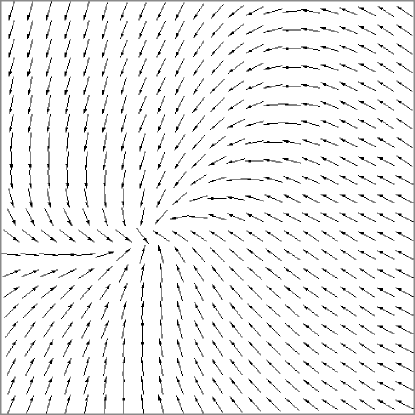
FIG. 1.: Field distribution at $t=0$.

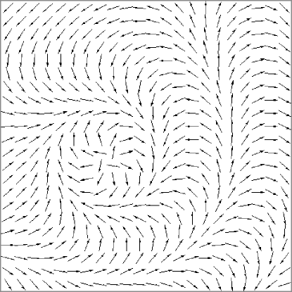
FIG. 2.: Field distribution at $t=20$ in the model (50) with $a=1$ and $c=-0.5$.

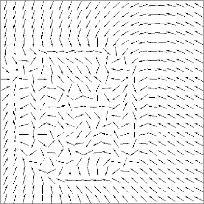
FIG. 3.: Field distribution at $t=0.3$ in the model (50) with $a=1$ and $c=-2$.

REFERENCES

- [1] A. T. Winfree, When Time Breaks Down (Princeton University Press, Princeton, 1987); V. S. Zykov, Simulation of Wave Processes in Excitable Media (Manchester University Press, Manchester, 1987).
- [2] A. V. Panfilov, Chaos 8, 57 (1998).
- [3] G. K. Moe, W. C. Rheinboldt, and J. A. Abildskov, Am. Heart. J. 67, 200 (1964).
- [4] R. Plonsey and R. C. Barr, Med. Biol. Eng. Comp. 24, 130, 137 (1987); W. Krassowska, T. C. Pilkington, and R. E. Ideker, IEEE Trans. Biomed. Eng. 34, 555 (1987); more recent work is reviewed by J. P. Keener, Chaos 8, 175 (1998); V. Krinsky and A. Pumir, ibid., p. 188; B. J. Roth and W. Krassowska, ibid., p. 204; N. Trayanova, K. Skouibine, and F. Aguel, ibid., p. 221.
- [5] R. FitzHugh, Biophys. J. 1, 445 (1961).
- [6] J. Rinzel, J. Math. Biol., 5, 363 (1978); J. Rinzel and J. P. Keener, SIAM J. Appl. Math. 43, 907 (1983).
- [7] C. F. Starmer et al., Biophys. J. 65, 1775 (1993).
- [8] Visualization of the lattice field was done using the program DynamicLattice from Cornell, see http://www.lassp.cornell.edu/LASSPTools/LASSPTools.html.
- [9] I. Aranson, L. Kramer, and A. Weber, Phys. Rev. Lett. 72, 2316 (1994); H. Chaté and P. Manneville, Physica A 224, 348 (1996).