Time-dependent calculation of ionization in Potassium at mid-infrared wavelengths

Abstract

We study the dynamics of the Potassium atom in the mid-infrared, high intensity, short laser pulse regime. We ascertain numerical convergence by comparing the results obtained by the direct expansion of the time-dependent Schrödinger equation onto $B$-Splines, to those obtained by the eigenbasis expansion method. We present ionization curves in the 12-, 13-, and 14-photon ionization range for Potassium. The ionization curve of a scaled system, namely Hydrogen starting from the 2s, is compared to the 12-photon results. In the 13-photon regime, a dynamic resonance is found and analyzed in some detail. The results for all wavelengths and intensities, including Hydrogen, display a clear plateau in the peak-heights of the low energy part of the Above Threshold Ionization (ATI) spectrum, which scales with the ponderomotive energy $U_{p}$, and extends to $(2.8\pm 0.5)U_{p}$.

I Introduction

The motivation for this work has its origin in recent experimental data by DiMauro et al [1] who studied high order harmonic generation (HOHG) and above threshold ionization (ATI) in potassium driven by strong radiation in the wavelength range 3200–3900 nm. Although HOHG and ATI have been and continue to be studied extensively, the bulk of the data and theory have concentrated on the noble gases. Experimental convenience has been one of the reasons for this preference, but, at least as far as HOHG is concerned, their relatively high ionization potentials and resistance to ionization have also tilted attention in their direction. The alkali atoms belong to an entirely different class, when it comes to their behavior under strong field excitation. For atomic numbers comparable to the respective noble gas (potassium versus argon in our context), their ionization potential is lower by more than a factor of three. Their excited states and distribution of the oscillator strength for transitions from the ground state are also considerably different. The energy of the first excited state in potassium is much closer to the ground state than it is in argon. As a consequence, if we consider, for example, 12-photon ionization in potassium, five of the photons reach above the first excited state, and the rest seven must be absorbed within the manifold of its excited states. In contrast, for 12-photon ionization of argon, it takes nine photons to reach the energy range of the first excited state and only the remaining three will involve excitation within the manifold of excited states. In addition, the wavelength needed for potassium (about 3000 nm) is longer by a factor of three than that needed for argon (about 1100 nm).

One might thus expect that, in the process of ionization, an extensive manifold of excited and Rydberg states will be strongly driven and perhaps populated. This should lead to a structure in the ATI energy spectrum different in appearance from what we are accustomed to. One might also anticipate that the behavior should have similarities with that observed in Rydberg states driven by microwave fields. Resolution requirements in photoelectron energy analysis do not allow the observation of individual ATI peaks in that case, although it is quite feasible to resolve such peaks in potassium driven from its ground state by radiation at mid-infrared wavelengths; as Sheehy et al. [1] have shown. It is the exploration of possible links and similarities between these two situations that induced us to undertake this work. Clearly, the requirements on intensity for saturation are expected to be lower in potassium than in argon. Moreover, given the expected participation of manifolds of excited states in potassium, the Keldysh parameter as a criterion for the departure from multiphoton ionization may not be as valid as it should be in argon where most of the energy interval from the ground state to the continuum is empty of excited states; imitating thus better the Keldysh model which is essentially based on a ground state and an ionization threshold.

The outline of this paper is as follows: The theory, namely the model used to describe the atom, and the two propagation methods used to solve the time-dependent Schrödinger equation are briefly presented in section (II). Section (III), starts with a presentation of the parameter range of the simulations that follow and a demonstration of convergence by comparing two different methods. It then moves on to present results in the 12-, 13-, and 14-photon ionization range, and discuss a low-energy plateau in the ATI spectrum. 12-photon ionization of Hydrogen starting from the 2s is compared to the results from Potassium. We conclude in section (IV), by summarizing the main findings of our results. In the appendix we present some details of the atomic structure model, and compare it with an alternative approach.

II Method

Potassium, being an alkali atom, can be considered a single electron system for most of the phenomena in which double excitation does not play an essential role. The first ionization threshold is about 4.34 eV above the ground state; 18.8 eV are needed to reach the lowest doubly excited state, which leaves us with enough room to study single electron dynamics. The simplest way to do this is by using a model potential that incorporates the effect of the core electrons, and thus reduces the dynamics to a single electron scheme. Different implementations of this basic idea have been used so far, with some success, in the Single Active Electron approach, pioneered by Kulander [2], the frozen core calculations [3], and other model potential calculations [4]. For the purpose of studying the dynamics in the mid-infrared, it is sufficient to use a simple form of the potential, proposed by Hellmann [5], which in atomic units is given as:

$$V_{m}=-\frac{1}{r}+A\frac{e^{-Kr}}{r},$$ (1)

where $A$ is 1.989 and $K$ is 0.898. All formulas that follow are given in atomic units. The Hellmann potential with the above mentioned parameters, results in a ground state energy of 38950 wavenumbers from the first ionization threshold, which is lower than the energy of the actual ground state (35010 wavenumbers) by 11%. Owing to the difference between the ground state energies of the model potential and of the real atom, we also use a scaled wavelength, namely we rescale the energy of the photon needed in an experiment that studies the same process, by the ratio of the model to the theoretical ground state energy. An alternative approach is to correct the energy of the ground state, and probably some matrix elements to satisfy the oscillator strength sum rules, but this leads to nonlocal modifications in the Hamiltonian and is difficult to implement effectively when the propagation is not done in an eigenbasis expansion.

The dynamical part of the problem is treated by solving the resulting time-dependent Schrödinger equation in the dipole approximation:

$${\mathrm{i}}\partial_{t}\Psi(\mbox{\boldmath{$r$}},t)=\left[H_{a}+D(t)\right]\Psi(\mbox{\boldmath{$r$}},t),$$ (2)

where $\Psi$ is the wavefunction describing the outer electron, and depends on the spatial electronic coordinates and on time, $H_{a}$ is the time-independent field-free atomic Hamiltonian, and $D(t)$ is the dipole interaction of the atom with the field. We only use the velocity form of the interaction operator, following detailed studies on the convergence properties of the solution [6], which have shown that the expansion of the wavefunction in terms of spherical harmonics can be shortened dramatically if the velocity gauge is used instead of the length gauge. In the velocity gauge, the dipole operator can be cast in the following form:

$$D(t)=-\alpha{\mbox{\boldmath{$A$}}(t)}\cdot\mbox{\boldmath{$p$}},$$ (3)

where $\alpha$ is the fine structure constant, $p$ is the momentum operator, and ${\mbox{\boldmath{$A$}}(t)}$ is the vector potential which, within the dipole approximation, has no spatial dependence. We choose a convenient form for the pulse envelope, namely a $\cos^{2}$, avoiding the long tails of a Gaussian that make the numerics more difficult, without significantly affecting the results. The explicit form is:

$$A(t)=\frac{{\cal E}_{0}}{\omega}\cos(\frac{\pi t}{\tau})^{2}\cos(\omega t),\quad\text{with }t\in[\frac{-\tau}{2},\frac{\tau}{2}],$$ (4)

where $A(t)$ is the amplitude of the vector potential, $\tau/2$ is the Full Width at Half Maximum (FWHM), ${\cal E}_{0}$ and $\omega$ the maximum field strength and fundamental frequency respectively. The solution of the resulting time-dependent equation is written in a system of spherical coordinates and expanded in terms of radial functions and angular spherical harmonics. This choice is dictated by the central symmetry of the atomic system and has the advantage of requiring the discretization of only one coordinate. Note that this choice leads to efficient algorithms only if the linearly polarized field is not too strong (compared to the coulomb field) in which case the global symmetry of the entire system would rather be cylindrical. Writing the solution in the cylindrical system would require discretization of 2 coordinates [7] greatly increasing the numerical cost of the algorithm. The problem is therefore treated within ”a box” (a sphere in the present case) whose radius is chosen sufficiently large to contain the expanded atom during the interaction. Part of the procedure for testing convergence consists in ascertaining that the ATI spectrum is insensitive to the radius of the box.

We have used two methods of propagating the TDSE, namely a propagation onto eigenstates in a box [8, 9], and a propagation on a $B$-Splines basis [6, 10]. The expansion of the time-dependent wavefunction on an eigenbasis set reads:

$$\Psi(t)=\sum_{l,n}b_{l,n}(t)\Phi^{l}_{n(E)},$$ (5)

where $\Phi^{l}_{n(E)}$ are the field-free box eigenstates of the atom of angular momentum $l$. Since we use linearly polarized light, we only need the $m=0$ magnetic quantum number, as the initial state has $m=0$, and dipole transition selection rules forbid mixing of other magnetic sublevels. The time-dependent Schrödinger equation is transformed into:

$$\mbox{i}\frac{d}{dt}b_{l,n}(t)=\sum_{n^{\prime}l^{\prime}}(E_{nl}\delta_{nn^{\prime}}\delta_{ll^{\prime}}-D_{nl,n^{\prime}l^{\prime}}(t))b_{l^{\prime},n^{\prime}}(t),$$ (6)

with the initial condition $|b_{l=0,n=1}(0)|^{2}=1$. $E_{nl}$ are the eigenvalues in the box; $D_{nl,n^{\prime}l^{\prime}}$ are the dipole matrix elements. Thus the problem has been transformed to a set of ordinary differential equations for the coefficients $b_{l,n}(t)$ of the wavefunction, which are solved using a high order, explicit propagation technique, namely a fifth-order and sixth-order Runge-Kutta-Verner method. The ionization yield is calculated by adding up the occupation probabilities of all discretized continuum states at the end of the pulse; the above threshold ionization (ATI) spectrum is obtained by the window operator projection technique [11, 12]. Bound state populations are given directly by the square of the norm of the coefficients of equation (5). For the construction of the box-eigenstates that are used as our basis, we use an expansion onto $B$-Splines, a method that is gaining momentum in many parts of atomic physics as was pointed out in [13]. The codes we use are based on ideas published in [3, 8], which have been expanded to accommodate the need for large boxes. It should be stressed that after the basis has been constructed (i.e. energies and matrix elements have been calculated), the rest of the procedure is neutral to the technique for the construction of the basis.

The second approach rests on expanding the radial part of the time-dependent wavefunction directly onto $B$-splines [6, 10]:

$${\Psi({\mbox{\boldmath{$r$}}},t)}={\sum\limits_{il}}b_{i}^{l}(t)\frac{B_{i}^{(k)}(r)}{r}{\mathrm{Y}_{lm}(\theta,\phi)}$$ (7)

where in addition to the spherical harmonics, $B_{i}^{(k)}(r)$ is the $i$-th $B$-spline of order $k$ depending only on the radial coordinate and $b_{i}^{l}(t)$ are time-dependent coefficients to be determined by the solution of the TDSE. Again, only $m=0$ magnetic quantum numbers are relevant. The major difference in this approach is that we need not prediagonalize anything other than the initial state. Substitution of equation (7) into the Schrödinger equation (2) leads to a banded system of differential equations, which is solved by implicit propagation techniques, currently involving a Bi-conjugate gradient method with preconditioner. This second method of propagation scales only linearly with increasing box size: it is thus more efficient when we need a large box. Although our original exploratory calculations have been made with the eigenbasis expansion method, which works quite well for small boxes, most of the results presented in what follows have been obtained through the direct expansion of the time-dependent Hamiltonian onto $B$-Splines.

III Results & Discussion

A General Considerations

The only guideline as to what to expect in our study are the experimental data by Sheehy et al. [1], in which 12-, 13-, and 14-photon ionization of Potassium has been studied, with 3.2 $\mu$m, 3.6 $\mu$m, and 3.9 $\mu$m, 1.5 ps pulses respectively, and intensities close to saturation. The 1.5 ps pulse is computationally impractical in the TDSE framework, thus we have chosen to place our study in the short pulse regime, with the total pulse duration $\tau$ of the $\cos^{2}$ pulse being 20 optical cycles, which (depending on the wavelength) corresponds to a width of 96 fs to 136 fs for the results that we present. The wavelengths we use are scaled, to compensate for the inaccuracy of the ground state energy, and are such that 12-, 13- and 14-photon ionization takes place. An intensity range estimate is obtained by calculating the generalized cross-section through a scaling technique [14, 15], using the energy (0.295 Hartree), and radius (5.24 a.u.) obtained with the general Hartree-Fock code published by Froese-Fischer [16]. From the cross-section, we obtain a saturation intensity estimate by solving $\Gamma t_{\text{eff}}=1$, where $\Gamma$ is the ionization width, and $t_{\text{eff}}$ an effective pulse duration, of the order of its FWHM [17]. After the first time-dependent calculations, it was established that scaling was underestimating saturation intensity by more than an order of magnitude. We also calculate the Ammosov, Delone, Krainov (ADK) rate of tunneling ionization [18], which does not depend on the wavelength. Solving $\Gamma t_{\text{eff}}=1$, we obtain a saturation intensity estimate of about $4\times 10^{12}$ W/cm², in agreement with the results of the simulations.

For some characteristic wavelengths, corresponding to 12-photon ionization scaled from the experimental wavelength, and the limits of the 13-photon ionization range, we show, in table (I), the FWHM duration $\tau/2$, the scaled-theory saturation intensity I_s, the ADK theory saturation intensity estimate I_ADK, and the upper limit E_c of the converged ATI spectrum for a 3000 atomic units box. E_c is calculated by estimating the energy needed for a free electron originally placed at the nucleus to reach the boundary of the box during the pulse; it is a useful simple estimate of the box size needed to study ATI spectra, as has been shown in section (5) of [10]. Next, and for two intensities, we show the ponderomotive energy $U_{p}$, which is the major component of the shift of the Rydberg states and the continuum [19, 20, 21]. It is given by:

$$U_{p}=\frac{I}{4\omega_{0}^{2}}\sim I\lambda^{2}$$ (8)

where $I$ is the laser intensity, $\omega_{0}$ the photon energy and $\lambda$ the corresponding wavelength. For the highest intensities that we use, the ponderomotive energy is a multiple of the photon energy, which is around a third of an eV for the wavelengths in the table. We also present the Keldysh tunneling parameter $\gamma$ [23], defined by:

$$\gamma^{2}=\frac{I_{p}}{2U_{p}}$$ (9)

where $I_{p}$ is the ionization potential, and $U_{p}$ the ponderomotive potential. Note that for all wavelengths, and for intensities up to $2\times 10^{12}$ W/cm², $\gamma$ is larger than one. Thus, according to the Keldysh theory of tunneling ionization, the process lies in the multiphoton regime, and it is meaningful to refer to the order of the transitions involved.

TABLE I.: Parameters for some of the calculations in Potassium.

$\lambda(nm)$	$\tau/2(fs)$	$I_{\mathrm{s}}$(W/cm2)	$I_{\mathrm{ADK}}$(W/cm2)	$E_{\mathrm{c}}(eV)$	$I$(W/cm2)	$U_{p}(eV)$	$\gamma$
$2880$	$96$	$1.5\times 10^{11}$	$4.1\times 10^{12}$	$7.76$	$10^{11}$	$0.073$	$5.23$
					$10^{12}$	$0.733$	$1.65$
$3125$	$104$	$1.3\times 10^{11}$	$4.0\times 10^{12}$	$6.59$	$10^{11}$	$0.086$	$4.82$
					$10^{12}$	$0.863$	$1.52$
$3300$	$110$	$1.2\times 10^{11}$	$4.0\times 10^{12}$	$5.91$	$10^{11}$	$0.096$	$4.56$
					$10^{12}$	$0.961$	$1.44$

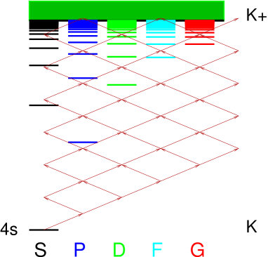
FIG. 1.: Truncated atomic structure of Potassium (calculated by the Hellmann potential), and quantum paths leading to 13-photon ionization

In figure (1) we show a visual representation of Potassium in a 3300 nm field, corresponding to the lowest energy photons in the 13-photon ionization range. A truncated part of the bound atomic levels, of angular momentum up to 4, is shown, together with the quantum paths leading to 13-photon ionization. Graphs of this type prove to be useful tools in the qualitative analysis of the processes involved in multiphoton phenomena.

In our study, we analyze the wavefunction at the end of the pulse, and thus obtain information on the electron spectrum and ionization. Depending on the physical quantity we are looking for, the parameters needed to achieve convergence vary, making it easier to obtain the value of angle and energy integrated ionization, than the ATI spectrum. We have ensured the convergence of our results, by varying the box size and the grid sampling density, in a way similar to what has been presented in [10], and by relying on empirical findings such as the definition of E${}_{\text{c}}$, or the needed density of discretized continuum states per photon energy, to guide our parameter choice. We have in addition conducted a further independent test of the numerics involved, by comparing the two different methods, i.e.  the expansion in terms of box-eigenstates, or the direct expansion of the radial part in a $B$-Splines basis. A sample result, for a demanding quantity such as the ATI spectrum in the 13-photon range, is shown in figure (2), where the results of the two simulations at 3300 nm, $7\times 10^{11}$ W/cm² and 110 fs are displayed on top of each other. The direct $B$-Splines method involves a box of 3000 a.u., with 3000 linearly sampled $B$-splines of order 7, for each angular momentum up to $l=20$, parameters that have proven more than sufficient for the method to converge in the range shown. After the propagation is over, a projection to scattering states is used to obtain the ATI spectrum. The eigenstates expansion involves a box of 2500 a.u., with 2500 linearly sampled $B$-Splines of order 9 for each angular momentum up to $l=15$ for constructing the eigenbasis. This basis was then truncated to the lowest 1000 basis elements per angular momentum; using only the 1000 lowest states proved to be sufficient for the energy range presented here, since the higher energy discretized continuum states play a role in the high energy, low-yield part of the spectrum. The window-operator technique [11] was used to obtain the photoelectron spectrum after the simulation, and the spectrum was renormalized for the comparison with the $B$-Splines spectrum.

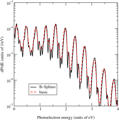
FIG. 2.: Two different, time-dependent methods of calculation of the dynamics of the Potassium model potential, for a 3300 nm, $7\times 10^{11}$ W/cm², 110 fs, $\cos^{2}$ pulse. The full line is the ATI spectrum obtained through the $B$-splines expansion method, and the dashed line is the ATI spectrum obtained through the eigenbasis calculation.

Despite the differences in the methods used, we observe an excellent agreement of the results in figure (2), even on a logarithmic scale. The $B$-Splines method shows richer structure at the minima between the peaks, demonstrating its superiority at the finest parts of the results. In detailed analysis of the ATI results (too long to be presented here), we have studied the behavior of the side peaks with intensity and we have noted that different peaks show different shifts with intensity, which helps us in classifying them as either Freeman resonances [24] or Bardsley fringes [22, 6]. Note further the clean formation of a plateau in the ATI-peak heights, showing up in both methods, and extending over the first 5 to 6 peaks; we study this plateau later in the paper. Since, in theory, the two methods are related by a unitary transformation of the basis from a spatially localized ($B$-Splines) to a field-free diagonal (eigenbasis) representation, the agreement of the results is expected; however, practice has shown that convergence is strongly affected by the underlying numerics, especially when it comes to ATI spectra that stress the subtle parts of our codes. It is the first time we have used such an elaborate procedure to ascertain the accuracy of our results. All results presented from now on are from calculations with the direct expansion onto $B$-splines, which is more efficient both in computer space and time, when the scale of the simulation increases. We have compared the results of both methods for all intensities at 3300 nm (13-photon range) and some intensities in the 12-photon range (2880 nm). The convergence of all other calculations presented was ensured within the $B$-Splines propagation method only, using well documented techniques [10]: variation of box-size, $B$-Splines density and order, and variation of the number of angular momenta.

B Behavior of ion yields as a function of intensity

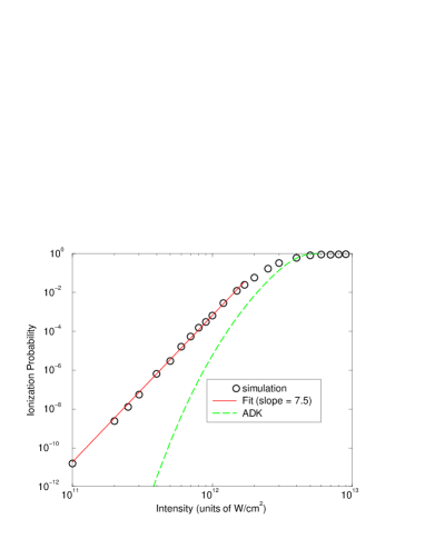
FIG. 3.: The ion yield versus intensity, and a fit of the low-intensity data to a power law. A 2880 nm, 96 fs, cos ² pulse is used. The dashed line shows the ADK-theory prediction.

We begin the presentation of our results with a study of ion yields, beginning with the 12-photon process at a 2880 nm pulse, of 96 fs temporal width, and intensities ranging from $10^{11}$ W/cm² to $10^{13}$ W/cm². A 2000 a.u. box with 2000 linearly sampled $B$-Splines of order 7, for each angular momentum up to $l=20$, proves sufficient for obtaining the ion yield. In figure (3) we present the results, together with a power-law fit to the low-intensity part of the spectrum. In the same figure we also show the ionization yield estimate obtained by the ADK-theory: in this and the following figures where the ADK predictions are displayed, we have integrated the ADK-rate over a square pulse of maximum intensity equal to the FWHM of the pulse used. Saturation sets in at about $3\times 10^{12}$ W/cm², substantially higher than the scaled estimate of $10^{11}$ W/cm², and in very good agreement with the ADK prediction. The low-intensity spectrum seems to follow a multiphoton perturbative behavior, in agreement with the value of the tunneling parameter $\gamma$ in table (I), and thus the power-law; but the least squares fit yields a slope of 7.5, substantially smaller than the lowest-order perturbation theory expectation of 12. The same behavior appears in the experimental results [1], where in the 12-photon ionization curve, a slope of 7 has been measured. Note that the ADK-theory, which is often used in comparisons to experiments due to its simplicity, markedly fails to predict the low-intensity yield.

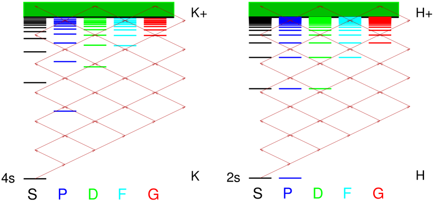
FIG. 4.: Potassium under 2880 nm radiation (left), and Hydrogen starting from the 2s under 4090 nm radiation (right). A truncated part of the atomic structure is shown, together with the quantum paths leading to ionization.

A scaled system, namely the 12-photon ionization process in Hydrogen starting from the metastable 2s state and interacting with 4090 nm light, is used as a test for these results. These two different systems are compared in figure (4), where we show bound states of Potassium and Hydrogen for the 4 lowest angular momenta, together with the 12-photon quantum paths leading to ionization, in energy units scaled to the photon energy. The 2s state is chosen instead of the ground state of Hydrogen as the initial state, so that the ionization threshold energy and the distribution of the bound states, other than the degeneracies, resemble those of Potassium.

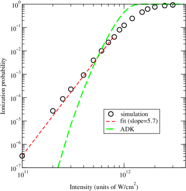
FIG. 5.: Ion yield for Hydrogen starting from the 2s in the 12-photon regime, and a fit of the low-intensity part to a power law. A 4090 nm, 136 fs, cos² pulse is used. The dashed line shows the ADK-theory prediction.

The resulting ion yield for a 136 fs pulse is shown in figure (5). A 3500 a.u. box with 3500 linearly sampled $B$-Splines of order 7 for each of the 21 angular momenta is used; this is certainly an overkill just for obtaining the ionization spectrum, but we also analyzed the ATI spectra which need such large boxes due to the long propagation times involved. We see the same kind of structureless saturated spectrum; albeit this time the yield is higher for the same intensities (notice the scales in the figures), and the saturation intensity is smaller by a factor of 2, in accordance with the scaling relations that predict a higher cross-section for Hydrogen starting from the 2s. The ADK theory (shown as the dashed line in the figure) departs at the lower part of the spectrum, and predicts a smaller saturation intensity. The low-intensity part again shows a linear dependence in the log-log plot, and this time the slope is 5.7, even less than what it is in Potassium. The slopes in both Potassium and Hydrogen 2s, roughly equal the order needed to ionize from the first exited state, the 4p and 3s or 3d respectively, yet, no unambiguous model conforming to all of our data could be constructed. Working in a related context, Pont et al. [25] have constructed a theory describing multiphoton ionization in a strong field of low frequency $\omega$, obtaining an asymptotic expansion of the ac quasienergy in powers of $\omega^{2}$. Their paper contains results for the rate of ionization from the 1s state of hydrogen in a circularly polarized 1064 nm field. When translated into a log-log plot of the rate vs intensity, the rate seems to increase roughly like the eighth power of the intensity, instead of the twelfth power as should be expected if the rate was perturbative.

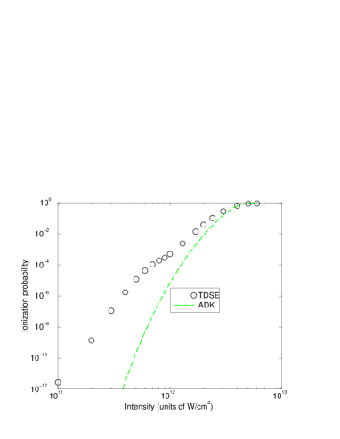
FIG. 6.: Ion yield versus intensity. A 3300 nm, 110 fs, cos² pulse is used. The dashed line shows the ADK-theory prediction.

We move on to 13-photon ionization, where the spectrum shows an unexpected feature. In figure (6) we show the ion yield versus intensity, using 3300 nm, 110 fs pulses, calculated within a box of 3000 a.u. with 3000 $B$-Splines per angular momentum up to $l=20$; for comparison we also display the predictions of the ADK theory. The saturation intensity is similar to the one in the 12-photon case, and again a power-law behavior of the signal with intensity holds for the lowest intensities. We observe, however, a “knee” in the ion-yield curve, for intensities around $8\times 10^{11}$ W/cm². This feature resembles a dynamic resonance, rather unexpected given the very high order of the processes involved.

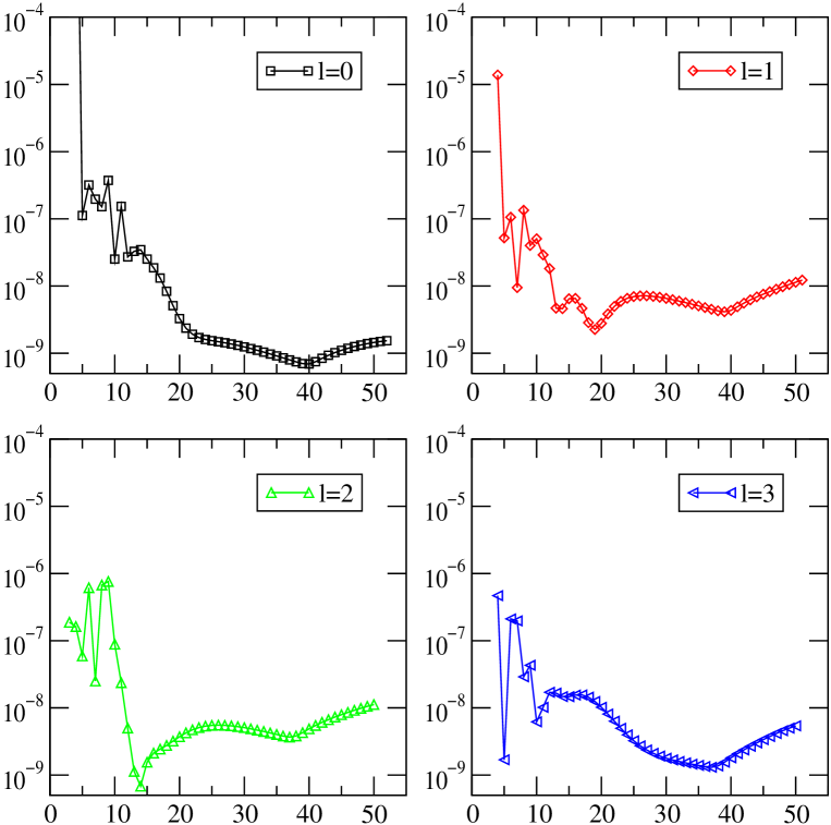
FIG. 7.: Bound state distribution at the end of a 3300 nm, 110 fs, cos² pulse. We present the population probability of bound states with respect to their main quantum number, for the four lowest angular momenta $l$. The lines have no physical meaning, and are only meant as a guide to the eye.

In figure (7) we plot the distribution of the final bound states for an intensity of $7\times 10^{11}$ W/cm². We plot the population probability, versus the principal quantum number for a few of the lowest angular momenta. Most of the population is still in the ground state at this intensity; most of the excited population is concentrated in the $4p$ state, and this is true for all lower intensities. Structure appears in the low-angular momentum, low-excited states, then a smooth, flat part, and a bump at the highest excitations. This bump turns out to be artificial, created by the pseudostates lying between the true bound states and the discretized continuum states. This was confirmed by observing that by making the box smaller, and thus changing the number of supported bound states, the same effect always appeared in the region just before the continuum. The smooth region just before the bump is expected, given the small energy differences of these states, compared with the shifts experienced during the pulse.

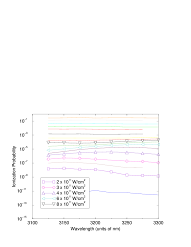
FIG. 8.: The ion yield versus wavelength is shown. A 20 cycles cos² pulse is used. We use boxes of 2000 a.u., with 2000 linearly sampled $B$-Splines of order 7, for each of the 21 lowest angular momenta.

In order to shed more light on the behavior of the “knee”, we performed a series of calculations, for different wavelengths, scanning the entire 13-photon range, from 3125 nm, to 3300 nm, with a step of 25 nm, and with pulses of 20 optical cycles, whose widths correspond to 104 fs for the 3125 nm wavelength, and to 110 fs for 3300 nm. In figure (8), we plot the ion yield as a function of the wavelength, for a series of intensities ranging from $10^{11}$ W/cm², to $3\times 10^{12}$ W/cm². The curves separate in a natural way, since for a fixed wavelength a higher intensity yields more ionization, and we note that for the highest intensities, above about $10^{12}$ W/cm², all wavelengths result in practically the same yield. In the graph we label only the intensities of interest that are in the range of 2–8$\times 10^{11}$ W/cm², where we see a broad resonance shifting to higher wavelengths with increasing intensity; this suggests a resonance shifting downwards by increasing the intensity.

In figure (9) we plot (for a few, selected wavelengths) the ionization curves, together with the total excitation, which is defined as the population in all bound states other than the ground state at the end of the pulse. The excitation is essentially dominated by the population of the 4p state, for most of the low- to mid-intensity range. Note the smooth variation of the curves with the wavelength; the results for the other wavelengths of figure (8), essentially interpolate the ones shown here. All curves exhibit a “knee” which is more pronounced in the excitation spectrum; after that, ionization mimics excitation in its behavior, whereas for the lower intensities — see especially 3150nm and 3200 nm — their behavior may differ substantially. One can argue that the low intensity part is typical in the multiphoton picture, where the difference in the orders of the processes involved is expected to show up as a difference in excitation compared to ionization. In a Floquet picture, few selected avoided crossings would describe the bulk of the dynamics. As the intensity increases, and higher excitations play a more important role, a regime is reached, where ionization and excitation are linked, similar to the transition to the classical chaos regime, which has been discussed in the microwave context, for example in [26].

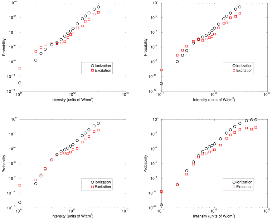
FIG. 9.: The ion yield and the total excitation for (left to right, and top to bottom) 3150, 3200, 3250, and 3300 nm radiation and a 20 cycles pulse. A box of 2000 a.u. is used.

For all wavelengths, and all intensities below the “knee”, the bound state distribution is qualitatively similar to the one in figure (7), with the 4p being by far the most populated excited state. On the basis of figure (1), this could happen assuming the shifts of the 4s and 4p to be such that the two states are brought closer together when the field is on. Indeed, by calculating the lowest order shift in the presence of the field and at the wavelengths of interest, it turns out that the 4s state shift is negative, and relatively small, whereas the 4p state, repelled by 5s, shifts down by more than three times as much. Thus, for the larger energy photons in the 13-photon range, a resonant excitation of the 4p state during the pulse occurs; for the lower energy photons of the same range, the shift pushes the states towards each other easing a near-resonant transfer. The phenomenon of a low excitation playing an essential role in a 13-photon ionization process, is easier to imagine in an atom like Potassium, than in Hydrogen starting from the ground state, since the excitation lies at less than half the energy that is needed to reach ionization. It should be noted here that 13-photon ionization simulations in Hydrogen, starting from the 2s at a scaled 13-photon wavelength of 4474 nm, display no corresponding characteristic, which can be attributed to the difference in the lowest excitation, as figure (4) shows.

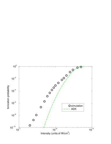
FIG. 10.: The ion yield for a 14-photon ionization process. A 3510 nm, 117 fs, cos² pulse is used. The dashed line shows the ADK theory prediction.

We close our discussion of ionization curves, by presenting in figure (10) the results of 14-photon ionization calculations, at a 3510 nm wavelength, with a 117 fs pulse. A 3000 a.u.  box was used, with 3000 $B$-Splines of order 7 per angular momentum, up to angular momentum $l=20$. We also present the ADK theory predictions: the departure at the lower intensities is not so dramatic as it was at the shorter wavelengths.

C Photoelectron energy spectra and ATI

We move on to the presentation of the ATI spectra, which, as seen in figure (2), exhibit a clean plateau in the low energy range. This plateau shows up at all wavelengths we have checked, in Potassium as well as in the Hydrogen simulations starting from the 2s, and it may thus be considered a global feature for mid-infrared wavelengths. In figure (11) a series of ATI spectra at 3300 nm, 110 fs $\cos^{2}$ pulses, and for selected intensities between $10^{11}$ W/cm² and $10^{12}$ W/cm² is shown; the higher the intensity, the higher the signal shown in the figure. A box of 3000 a.u., with 3000 $B$-splines of order 7 for each of the angular momenta up to $l=20$ is used. The vertical axis in the figure corresponds to the ionization probability density in units of 1/eV. The shift of the ATI peaks to lower energies with increasing intensity is linear with intensity, and, as expected, is well described by the ponderomotive shift of the ionization threshold. We note that the extent of the plateau grows, almost in proportion to the intensity.

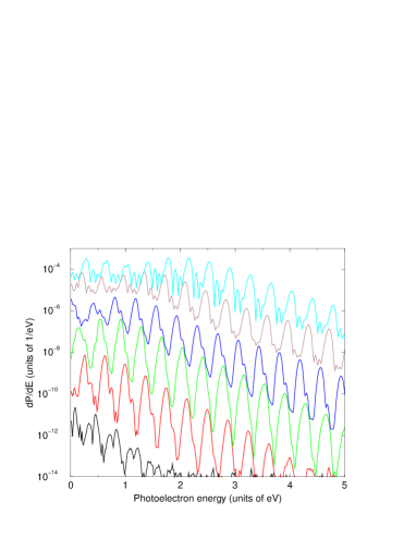
FIG. 11.: ATI spectra for (bottom to top) 1, 2, 3, 4, 6, $9\times 10^{11}$ W/cm². A 110 fs, 3300 nm, cos² pulse is used.

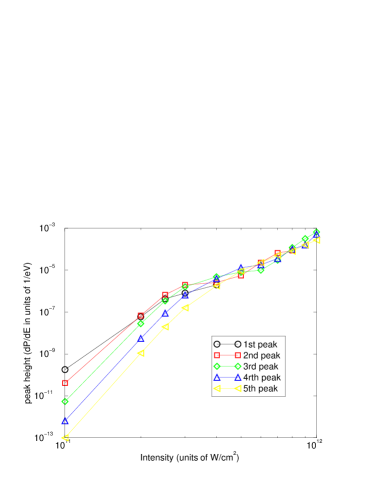
FIG. 12.: The height of the first few ATI peaks as a function of intensity. A 3150 nm, 100 fs, cos² pulse is used. The lines have no physical meaning and are only used as a guide to the eye. We notice the convergence of the peaks which indicates the plateau formation.

A clearer way of viewing this phenomenon is presented in figure (12). We plot the height of the first few ATI peaks versus the intensity of the pulse, this time for a 3150 nm wavelength and a width of 105 fs, corresponding again to a 20-cycle pulse. Note the power law (linear dependence on a log-log plot) of the first few peak-heights with the intensity. This indicates that a perturbative process is taking place. As the intensity increases, more peaks enter the plateau range and the perturbative picture ceases to hold. This is demonstrated in figure (12) by the merging of the curves, which implies that for a range of peaks their heights are basically the same. As the intensity increases, the plateau expands and more curves merge.

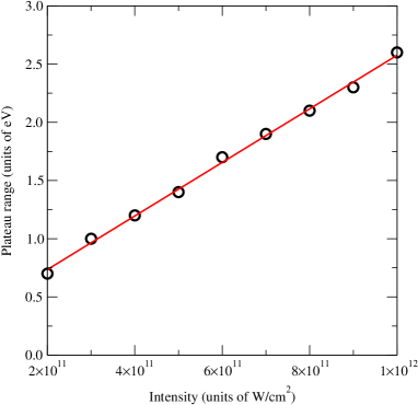
FIG. 13.: ATI spectra plateau range as a function of intensity. A 3300 nm, 110 fs, cos² pulse is used. Hand-read definition of plateau range.

In figure (13), we show the plateau range plotted versus the intensity for the calculation shown in figure (11). In this figure, the plateau range is defined as the abscissa of the interception of a horizontal line joining the first few peaks, and a line over the decreasing peaks of the spectrum. The fit was made by hand, to manually remove the effect of accidental resonances in the first peaks of the spectrum. We notice the sharp linear dependence of the plateau range on the intensity. On the same figure, we show a fit of the selected points to a linear function of intensity. The least squares fit gives a plateau range of $(2.3\times 10^{-12}\pm 4\times 10^{-14})$eV cm²/W$\times I+(0.28\pm 0.03)$eV. Measured in units of $U_{p}$ for the 3300 nm wavelength, the same equation reads: $(2.4\pm 0.04)U_{p}+(0.28\pm 0.03)$ eV. This shows a plateau scaling in proportion to $2.4U_{p}$.

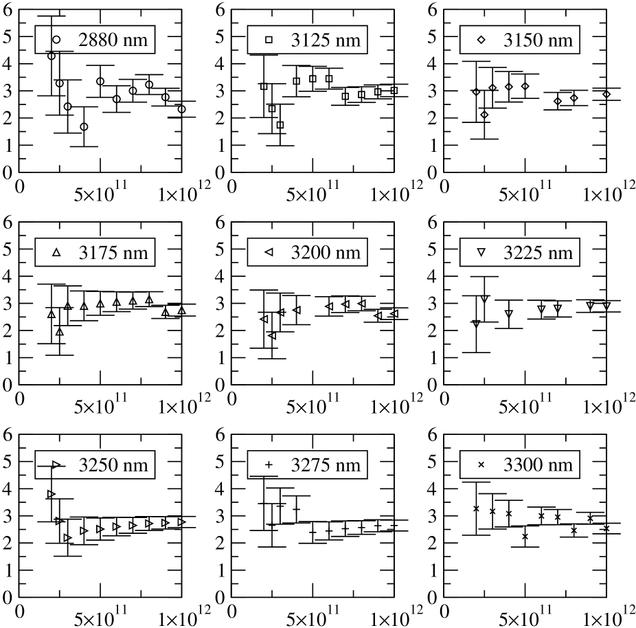
FIG. 14.: ATI spectra plateau range for a wealth of intensities and wavelengths. The horizontal axis shows the intensity in units of W/cm²; the vertical axis shows the extent of the plateau in units of the ponderomotive energy. The large error-bars present in the lowest intensities originate from the rigorous definition of the plateau range described in the text.

To clarify the relation of the plateau to the ponderomotive energy, we combine all of the data from the simulations in the 12-, and 13-photon range. We simplify the definition of the extent of the plateau to a rigorous one, whose extraction from the data is automated, namely, we use the abscissa of the first peak at which the exponential fall of the peak heights begins. The results are shown in figure (14), where for each intensity the plateau range measured in units of $U_{p}$ is shown for all wavelengths. The error-bars reflect the imprecision due to cases in which the plateau ends between two consecutive peaks. From the definition of the plateau range that we use, it follows that the real plateau has the same probability to be located anywhere within our error-bars. Notice the huge uncertainty (larger than $U_{p}$) at small intensities which reflects the fact that $U_{p}$ is smaller than the peak spacing. At higher intensities, the ponderomotive shift grows until it is considerably larger than the peak-spacing, thus shrinking the error-bars to less than $U_{p}$. The data is fitted to a normal distribution with an average value of 2.8 $U_{p}$ and a standard deviation of 0.5 $U_{p}$.

This result relates to the classical theory of the ionization process, as has been first developed in the simpleman’s model [27, 28, 29]. The main arguments have recently been clearly restated in the appendix of [30], although in the context of a rescattering picture [31]. The idea rests upon a free-electron maximally gaining 3.17 $U_{p}$ within a field, returning to its original position. This happens within the first cycle, or the first period of the electronic motion, subsequent cycles lead to 2.4 $U_{p}$, and then to less until the maxima gradually converge to 2 $U_{p}$ over many cycles, and the average kinetic energy becomes $U_{p}$. A relevant study has been made more than 10 years ago by Gallagher in the microwave regime [28], where ionization of Na Rydberg states was studied, and the spectra were explained using the above mentioned theory. In that paper, a plot of the extend of the spectrum starting from the 40 s state of Na, shows approximate scaling with 3.45 $U_{p}$. An energy of $U_{p}$ should be subtracted when compared to short-pulse experiments, as the electrons do not keep the extra ponderomotive energy since they cannot sample the spatial gradient of the field. After the observation, in the optical regime, of the long-range plateau extending from 2 to 8 $U_{p}$ [32, 33], the theory has been extended to include backscattering from the nucleus, having thus provided answers to pertinent questions [31, 34]. It should be noted that other than the original Gallagher experiment, all of these experiments and theories exhibit a steep fall in the region up to $2U_{p}$, which then stabilizes or falls with a lower slope in the region from 2 to 8 $U_{p}$. This is in contrast to our findings in the mid-infrared regime that show a smooth, almost flat region in the low energy spectra, and an increased downward slope afterwards. Due to the numerical demands on convergence, in the present study we do not analyze the region up to and beyond 8 $U_{p}$, and cannot therefore establish the presence or not of a second plateau.

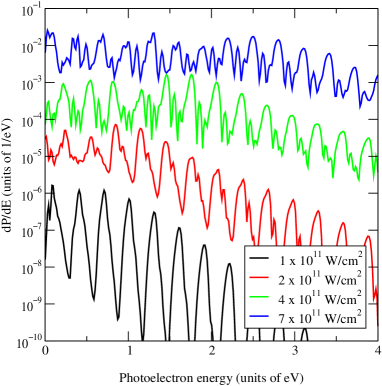
FIG. 15.: ATI spectra of Hydrogen starting from the 2s, in a 4090 nm field. The spectra for 1, 2, 4, and $7\times 10^{11}$ W/cm² are shown. A box of 3500 a.u.  with 3500 $B$-Splines per angular momentum is used.

We have also confirmed that the plateau characteristic has no relation to the atomic structure involved, by examining the ATI spectrum in the scaled problem, namely 12-photon ionization of Hydrogen starting from the 2s state. The data are from the simulations corresponding to the wavelength displayed in figure (4), and the parameters used are the same as those used to plot figure (5). Few selected ATI spectra are shown in figure (15), all of which display the plateau, whose range is estimated as $2.6\pm 0.3U_{p}$, close to what we obtained from the cumulative data in Potassium.

IV Conclusions

In summary, we have conducted a theoretical study of the dynamics of Potassium interacting with a high intensity, mid-infrared, short, laser pulse. We chose Potassium because it has recently been studied experimentally by Sheehy et al. [1]. We have performed time dependent calculations in terms of both a direct expansion of the Schrödinger equation onto $B$-Splines, as well as an expansion onto field-free eigenstates within a box, and obtained remarkable agreement between the two methods. We have studied a 12-photon ionization process, and have observed that the low-intensity, power-law behavior of the ion yield has an exponent much lower than the perturbative expectation of 12. We have obtained the same behavior from the study of a scaled system, namely Hydrogen starting from the 2s in the 12-photon range. In the 13-photon ionization of Potassium, we noted a “knee” structure in the ion yield, and linked it to a similar, more pronounced, behavior in the excitation. We interpret this feature as a broad dynamical resonance with the lowest excited state. The ATI spectra, in all cases that we have studied, display a clean formation of a plateau in the first few peak-heights. Although the extension of a plateau in the ATI spectrum at optical wavelengths from 2 to 8 times the ponderomotive energy has been discussed in the literature, the existence of a clear low-energy plateau has (to the best of our knowledge) not been observed in other studies in the optical or UV regime, but has been measured in the microwave regime and interpreted by the simpleman’s theory of ionization [28]. Through the analysis of the cumulative data from our simulations, we have determined the extent of the plateau to scale with the ponderomotive energy $U_{p}$ as $(2.8\pm 0.5)U_{p}$, which is compatible with the predictions of the classical theory. Given the much longer wavelength and therefore longer optical period, an initially launched wavepacket will have more time to spread before it backscatters from the core. This raises the question as to whether backscattering would play an important role at this wavelength. Recall that backscattering for shorter wavelengths has been associated with changes of the slope of the ATI spectrum up to around 10 $U_{p}$. A related question of course is whether the initially launched wavepacket might be narrower as a result of which their might not be substantial additional spreading by the time it reaches the core. A definitive evaluation of this aspect would require much more extensive calculations which may be worth undertaking in the future.

V Acknowledgements

We would like to thank Dr. L. F. DiMauro for making available their experimental results [1] prior to publication. Computer time, space and support from the Rechnenzentrum Garching, and especially John Cox and Dr. R. Volk is gratefully acknowledged. One of us (P. M.) would like to thank Dr. L. A. A. Nikolopoulos for useful discussions.

VI Appendix

In the appendix we discuss the model potential used, by comparing it to the accepted structure of Potassium and to the alternative frozen core Hartree-Fock model. The atomic structure of Potassium can be found in several places. Since we cannot in a straightforward manner incorporate relativistic effects in our theory, we use the weighted energy levels, which are calculated as:

$$E_{\text{av}}=\frac{1}{\sum\limits_{J_{i}}(2J_{i}+1)}\sum\limits_{J_{i}}(2J_{i}+1)E_{J_{i}}$$ (10)

The atomic eigenenergies $E_{J_{i}}$ are taken from [35]. For easier comparison with the numerical results, we measure the energies from the ionization threshold which is at 35009.814 wavenumbers according to Sugar and Corliss [36].

The multiplet oscillator strengths are calculated using the approximate formula [37]:

$$f_{ik}^{\text{multiplet}}=\frac{1}{\sum\limits_{J_{i}}(2J_{i}+1)}\sum\limits_{J_{i}J_{k}}(2J_{i}+1)f(J_{i},J_{k})$$ (11)

The data needed in this formula are taken from [35]. Note that in this database the quantity that is given is $\log((2J_{i}+1)f(J_{i},J_{k}))$. The multiplet oscillator strengths are shown in the second column of table (III). A few oscillator strengths are also presented in page 300 of [38]. They are in agreement with the ones shown in the table.

TABLE II.: Potassium energy levels measured from first ionization threshold. E${}_{\text{Exp}}$ (cm^-1) is the weighted nonrelativistic value, E${}_{\text{HF}}$ is the Frozen Core Hartree-Fock result, and E${}_{\text{H}}$ is the Hellman Potential value.

$State$	$E_{\text{Exp}}(cm^{-1})$	$E_{\text{HF}}(cm^{-1})$	$E_{\text{H}}(cm^{-1})$
$4s$	$-35010$	$-32253$	$-38947$
$5s$	$-13983$	$-13376$	$-15761$
$6s$	$-7560$	$-7326$	$-8331$
$4p$	$-21986$	$-20972$	$-22647$
$5p$	$-10296$	$-10000$	$-10696$
$6p$	$-6005$	$-5876$	$-6209$
$3d$	$-13474$	$-12755$	$-11952$
$4d$	$-7612$	$-7213$	$-6735$
$5d$	$-4824$	$-4600$	$-4322$
$4f$	$-6882$	$-6860$	$-6852$
$5f$	$-4403$	$-4390$	$-4384$
$6f$	$-3057$	$-3049$	$-3045$
$5g$	$-4393$	$-4390$	$-4389$

An alternative approach to the model potential, that originally seemed appealing, is the Frozen Core Hartree-Fock method. Its main merit is its ab initio nature, and the comparatively better description of atomic structure. Extensive theoretical discussion exists on the Frozen Core Hartree-Fock method. We used an implementation that is documented in [39]. The work in that paper was concerned with the application of the method to configuration interaction on the Frozen Core Hartree Fock basis, whereas here we are interested only in the single outer electron case. Atomic structure is described quite well, as we see in the third column of Table (II) where we show selected bound state energies, and in columns 3 and 4 of Table (III), where we present bound-bound oscillator strengths in the length and velocity gauge starting from s, p, and d states respectively. The energies are measured from the first ionization threshold and are expressed in wavenumbers for direct comparison with the available data. A 500 a.u. box, with 500 $B$-Splines of order 9 was used for the calculations. We notice that the agreement between oscillator strengths calculated in the length and velocity gauges is quite good for the cases displayed in the tables. The major disadvantage of the method is the inconvenient scaling of the time needed to calculate the basis, and the actual size of the basis calculated, which limits us to small cases, up to 1000 a.u.. The time needed by the frozen core Hartree Fock scales as $N^{4}$, although in principle it is limited by a $N^{3}$ factor. The size scales with $N^{2}$ per angular momentum, so that for a $N=3000$ basis of 20 angular momenta, we need approximately 2 GB and 35 CPU days in our workstation cluster to perform the structure calculations. Thus it is mainly numerical considerations that dictate the use of the pseudopotential method.

TABLE III.: Some Potassium multiplet oscillator strengths, starting from few lowest $s$, $p$, $d$ states. f is the exact multiplet oscillator strengths, f${}_{\text{HF}}$ is the Hartree-Fock result calculated in the length gauge, and f${}_{\text{H}}$ is the Hellmann potential result.

State	$f$	$f_{\text{HF}}(len)$	$f_{\text{HF}}(vel)$	$f_{\text{H}}$
$4s\rightarrow 4p$	$1.01$	$1.07$	$1.02$	$0.96$
$4s\rightarrow 5p$	$0.009$	$0.01$	$0.008$	$0.026$
$4s\rightarrow 6p$	$0.0009$	$0.0012$	$0.0008$	$0.0055$
$5s\rightarrow 5p$	$1.49$	$1.52$	$1.49$	$1.42$
$5s\rightarrow 6p$	$0.031$	$0.026$	$0.024$	$0.075$
$6s\rightarrow 6p$	$1.92$	$1.96$	$1.94$	$1.82$
$4p\rightarrow 5s$	$0.18$	$0.18$	$0.17$	$0.19$
$4p\rightarrow 6s$	$0.019$	$0.018$	$0.017$	$0.009$
$4p\rightarrow 3d$	$0.89$	$0.93$	$0.97$	$0.90$
$4p\rightarrow 4d$	$0.0003$	$0.012$	$0.015$	$0.092$
$4p\rightarrow 5d$	$0.003$	$0.0002$	$0.0005$	$0.028$
$5p\rightarrow 6s$	$0.31$	$0.32$	$0.31$	$0.34$
$5p\rightarrow 4d$	$1.20$	$1.25$	$1.29$	$1.00$
$5p\rightarrow 5d$	$0.0077$	$0.032$	$0.036$	$0.14$
$5p\rightarrow 6d$	$1.48\times 10^{-5}$	$0.0037$	$0.0046$	$0.048$
$3d\rightarrow 5p$	$0.14$	$0.16$	$0.18$	$0.14$
$3d\rightarrow 6p$	$0.0066$	$0.0066$	$0.0078$	$6.75\times 10^{-9}$
$3d\rightarrow 4f$	$0.76$	$0.88$	$0.88$	$1.061$
$3d\rightarrow 5f$	$0.17$	$0.16$	$0.16$	$0.14$
$3d\rightarrow 6f$	$0.067$	$0.062$	$0.062$	$0.049$
$4d\rightarrow 6p$	$0.30$	$0.34$	$0.35$	$0.25$
$4d\rightarrow 5f$	$0.39$	$0.17$	$0.17$	$0.97$
$4d\rightarrow 6f$	$0.14$	$0.62$	$0.62$	$0.18$

The last columns in tables (II), and (III) are the results of the Hellmann pseudopotential, as presented in equation (1), calculated with a box of 2500 a.u., with 2500 $B$-Splines of order 9. Since the potential is $l$-independent, length and velocity gauge oscillator strengths agree, without the need of introducing a correction to the dipole operator [40]. We calculated the standard deviation of the length and velocity absorption oscillator strengths starting from a specific state. For all bound states and up to the lower part of the continuum spectrum, which is what interests us, this was less than $10^{-5}$, which reassures us of the completeness of our description. The model potential represents the atom less accurately than the Hartree-Fock does, both energies and oscillator strengths. Nevertheless, its excellent numerical properties, originating from its simplicity, make the large calculations feasible. Scaling techniques help to map the model atom results onto real experiments, but our main aim is to study general features pertaining in the mid-infrared range, thus making the actual atom used of secondary importance.

REFERENCES

- [1] B. Sheehy, P. Agostini, and L. F. DiMauro, experimental measurements of ATI spectra and ion yields of Potassium in the mid-infrared region, private communication (unpublished).
- [2] K. C. Kulander, Phys. Rev. A 38, 778 (1988).
- [3] X. Tang, H. Rudolph, and P. Lambropoulos, Phys. Rev. A 44, R6994 (1991).
- [4] U. Lambrecht, M. Nurhuda, and F. M. Faisal, Phys. Rev. A 57, R3176 (1998).
- [5] L. Szasz, Pseudopotential Theory of Atoms and Molecules (Wiley-Interscience, New York, 1985).
- [6] E. Cormier and P. Lambropoulos, J. Phys. B 29, 2667 (1996).
- [7] P. Maragakis and P. Lambropoulos, Laser Physics 7, 679 (1997).
- [8] P. Lambropoulos, P. Maragakis, and J. Zhang, Phys. Reports 305, 203 (1998).
- [9] P. Lambropoulos, P. Maragakis, and E. Cormier, Laser Physics 8, 625 (1998).
- [10] E. Cormier and P. Lambropoulos, J. Phys. B 30, 77 (1997).
- [11] K. C. Kulander, K. J. Schafer, and J. L. Krause, in Atoms in Intense Laser Fields, edited by M. Gavrila (Academic Press, San Diego, 1992), pp. 247–300. See Ref. [12].
- [12] in Atoms in Intense Laser Fields, edited by M. Gavrila (Academic Press, San Diego, 1992).
- [13] J. Sapirstein and W. R. Johnson, J. Phys. B 29, 5213 (1996).
- [14] P. Lambropoulos, Phys. Rev. Lett. 55, 2141 (1985).
- [15] P. Lambropoulos and X. Tang, J. Opt. Soc. Am. B 4, 821 (1987).
- [16] C. F. Fischer, Comp. Phys. Comm. 43, 355 (1987).
- [17] D. Charalambidis, D. Xenakis, C. J. G. J. Uiterwaal, P. Maragakis, J. Zhang, H. Schröder, O. Faucher, and P. Lambropoulos, J. Phys. B 30, 1467 (1997).
- [18] M. V. Ammosov, N. B. Delone, and V. P. Krainov, Zh. Eksp. Teor. Fiz. 91, 2008 (1986), sov. Phys. JETP 64, 1191 (1986).
- [19] P. Avan, C. Cohen-Tannoudji, J. Dupont-Roc, and C. Fabre, Journal de Physique 37, 993 (1976).
- [20] M. H. Mittleman, Phys. Rev. A 29, 2245 (1984).
- [21] R. P. Freeman, T. J. McIlrath, P. H. Bucksbaum, and M. Bashkansky, Phys. Rev. Lett. 57, 3156 (1986).
- [22] J. N. Bardsley, A Szöke and M. J. Comella, J. Phys. B 21, 3899, (1988).
- [23] L. V. Keldysh, Sov. Phys. JETP 20, 1307 (1965).
- [24] R. H. Freeman, P. H. Bucksbaum, H. Milchberg, S. Darack, D. Schumacher, and M. E. Geusic, Phys. Rev. Lett. 59, 1092 (1987).
- [25] M. Pont, R. Shakeshaft, and R. M. Potvliege, Phys. Rev. A 42, R6969 (1990).
- [26] R. Blümel and U. Smilansky, Z. Phys. D 6, 83 (1987).
- [27] H. B. van Linden van den Heuvell and H. G. Muller, in Multiphoton Processes, edited by S. J. Smith and P. L. Knight (Cambridge Univ. Press, Cambridge, 1988), pp. 25–34.
- [28] T. F. Gallagher, Phys. Rev. Lett. 61, 2304 (1988).
- [29] P. B. Corkum, N. H. Burnett, and F. Brunel, Phys. Rev. Lett. 62, 1259 (1989).
- [30] K. J. LaGattuta and J. S. Cohen, J. Phys. B 31, 5281 (1998).
- [31] B. Walker, B. Sheehy, K. C. Kulander, and L. F. DiMauro, Phys. Rev. Lett. 77, 5031 (1996).
- [32] G. G. Paulus, W. Nicklich, H. Xu, P. Lambropoulos, and H. Walther, Phys. Rev. Lett. 72, 2851 (1994).
- [33] P. Hansch, M. A. Walker, and L. D. V. Woerkom, Phys. Rev. A 55, R2535 (1997).
- [34] B. Hu, J. Liu, and S. Chen, Phys. Lett. A 236, 533 (1997).
- [35] P. L. Smith, C. Heise, J. R. Esmond, and R. L. Kurucz, Atomic spectral line database from Kurucz files, 1995, http://cfa-www.harvard.edu/amdata/ampdata/kurucz23/sekur.html
- [36] J. Sugar and C. Corliss, Atomic Energy Levels of the Iron-Period Elements: Potassium through Nickel, No. Supplement No. 2 in Journal of Physical and Chemical Reference Data (American Chemical Society and American Institute of Physics, National Measurement Laboratory, National Bureau of Standards, Gaithersburg, Maryland 20899, 1985).
- [37] W. L. Wiese, M. W. Smith, and B. M. Miles, Atomic Transition Probabilities (U. S. Department of Commerce, National bureau of standards, 1969), Vol. 2.
- [38] I. I. Sobelman, Atomic Spectra and Radiative Transitions, Springer Series on Atoms+Plasmas, 2nd ed. (Springer-Verlag, Berlin, 1992).
- [39] T. N. Chang, in Many-body theory of Atomic Structure, edited by T. N. Chang (World Scientific, Singapore, 1993), pp. 213–247.
- [40] D. W. Norcross, Phys. Rev. A 7, 606 (1973).