NONLINEAR ACCELERATOR PROBLEMS VIA WAVELETS:
1. ORBITAL MOTION IN STORAGE RINGS

Abstract

In this series of eight papers we present the applications of methods from wavelet analysis to polynomial approximations for a number of accelerator physics problems. In this part, according to variational approach we obtain a representation for orbital particle motion in storage rings as a multiresolution (multiscales) expansion in the base of well-localized in phase space wavelet basis. By means of this ”wavelet microscope” technique we can take into account contribution from each scale of resolution.

1 INTRODUCTION

This is the first part of our eight presentations in which we consider applications of methods from wavelet analysis to nonlinear accelerator physics problems. This is a continuation of our results from [1]-[8], which is based on our approach to investigation of nonlinear problems – general, with additional structures (Hamiltonian, symplectic or quasicomplex), chaotic, quasiclassical, quantum, which are considered in the framework of local (nonlinear) Fourier analysis, or wavelet analysis. Wavelet analysis is a relatively novel set of mathematical methods, which gives us a possibility to work with well-localized bases in functional spaces and with the general type of operators (differential, integral, pseudodifferential) in such bases. In the parts 1-8 we consider applications of wavelet technique to nonlinear dynamical problems with polynomial type of nonlinearities. In this part we consider this very useful approximation in the case of orbital motion in storage rings. Approximation up to octupole terms is only a particular case of our general construction for n-poles. Our solutions are parametrized by solutions of a number of reduced algebraical problems one from which is nonlinear with the same degree of nonlinearity and the rest are the linear problems which correspond to particular method of calculation of scalar products of functions from wavelet bases and their derivatives.

2 Orbital Motion in Storage Rings

We consider as the main example the particle motion in storage rings in standard approach, which is based on consideration in [9]. Starting from Hamiltonian, which described classical dynamics in storage rings ${\cal H}(\vec{r},\vec{P},t)=c\{\pi^{2}+m_{0}^{2}c^{2}\}^{1/2}+e\phi$ and using Serret–Frenet parametrization, we have after standard manipulations with truncation of power series expansion of square root the following approximated (up to octupoles) Hamiltonian for orbital motion in machine coordinates:

$${\cal H}=\frac{1}{2}\cdot\frac{[p_{x}+H\cdot z]^{2}+[p_{z}-H\cdot x]^{2}}{[1+f(p_{\sigma})]}$$

$$+p_{\sigma}-[1+K_{x}\cdot x+K_{z}\cdot z]\cdot f(p_{\sigma})$$ (1)

$$+\frac{1}{2}\cdot[K_{x}^{2}+g]\cdot x^{2}+\frac{1}{2}\cdot[K_{z}^{2}-g]\cdot z^{2}-N\cdot xz$$

$$+\frac{\lambda}{6}\cdot(x^{3}-3xz^{2})+\frac{\mu}{24}\cdot(z^{4}-6x^{2}z^{2}+x^{4})$$

$$+\frac{1}{\beta_{0}^{2}}\cdot\frac{L}{2\pi\cdot h}\cdot\frac{eV(s)}{E_{0}}\cdot\cos\left[h\cdot\frac{2\pi}{L}\cdot\sigma+\varphi\right]$$

Then we use series expansion of function $f(p_{\sigma})$ from [9]: $f(p_{\sigma})=f(0)+f^{\prime}(0)p_{\sigma}+f^{\prime\prime}(0)p_{\sigma}^{2}/2+\ldots=p_{\sigma}-p_{\sigma}^{2}/(2\gamma_{0}^{2})+\ldots$ and the corresponding expansion of RHS of equations corresponding to (1). In the following we take into account only an arbitrary polynomial (in terms of dynamical variables) expressions and neglecting all nonpolynomial types of expressions, i.e. we consider such approximations of RHS, which are not more than polynomial functions in dynamical variables and arbitrary functions of independent variable $s$ (”time” in our case, if we consider our system of equations as dynamical problem).

3 Polynomial Dynamics

The first main part of our consideration is some variational approach to this problem, which reduces initial problem to the problem of solution of functional equations at the first stage and some algebraical problems at the second stage. We have the solution in a compactly supported wavelet basis. Multiresolution expansion is the second main part of our construction. The solution is parameterized by solutions of two reduced algebraical problems, one is nonlinear and the second is some linear problem, which is obtained from the method of Connection Coefficients (CC).

3.1 Variational Method

Our problems may be formulated as the systems of ordinary differential equations

$${\mathrm{d}x_{i}}/{\mathrm{d}t}=f_{i}(x_{j},t),\quad(i,j=1,...,n)$$ (2)

with fixed initial conditions $x_{i}(0)$, where $f_{i}$ are not more than polynomial functions of dynamical variables $x_{j}$ and have arbitrary dependence of time. Because of time dilation we can consider only next time interval: $0\leq t\leq 1$. Let us consider a set of functions $\Phi_{i}(t)=x_{i}{\mathrm{d}y_{i}}/{\mathrm{d}t}+f_{i}y_{i}$ and a set of functionals

$$F_{i}(x)=\int_{0}^{1}\Phi_{i}(t)dt-x_{i}y_{i}\mid^{1}_{0},$$ (3)

where $y_{i}(t)(y_{i}(0)=0)$ are dual variables. It is obvious that the initial system and the system

$$F_{i}(x)=0$$ (4)

are equivalent. In the following parts we consider an approach, which is based on taking into account underlying symplectic structure and on more useful and flexible analytical approach, related to bilinear structure of initial functional. Now we consider formal expansions for $x_{i},y_{i}$:

$$x_{i}(t)=x_{i}(0)+\sum_{k}\lambda_{i}^{k}\varphi_{k}(t)\quad y_{j}(t)=\sum_{r}\eta_{j}^{r}\varphi_{r}(t),$$ (5)

where because of initial conditions we need only $\varphi_{k}(0)=0$. Then we have the following reduced algebraical system of equations on the set of unknown coefficients $\lambda_{i}^{k}$ of expansions (5):

$$\sum_{k}\mu_{kr}\lambda^{k}_{i}-\gamma_{i}^{r}(\lambda_{j})=0$$ (6)

Its coefficients are

$$\mu_{kr} = \int_{0}^{1}\varphi_{k}^{\prime}(t)\varphi_{r}(t){\rm d}t,$$ (7)

$$\gamma_{i}^{r} = \int_{0}^{1}f_{i}(x_{j},t)\varphi_{r}(t){\rm d}t.$$

Now, when we solve system (6) and determine unknown coefficients from formal expansion (5) we therefore obtain the solution of our initial problem. It should be noted if we consider only truncated expansion (5) with N terms then we have from (6) the system of $N\times n$ algebraical equations and the degree of this algebraical system coincides with degree of initial differential system. So, we have the solution of the initial nonlinear (polynomial) problem in the form

$$x_{i}(t)=x_{i}(0)+\sum_{k=1}^{N}\lambda_{i}^{k}X_{k}(t),$$ (8)

where coefficients $\lambda_{i}^{k}$ are roots of the corresponding reduced algebraical problem (6). Consequently, we have a parametrization of solution of initial problem by solution of reduced algebraical problem (6). The first main problem is a problem of computations of coefficients of reduced algebraical system. As we will see, these problems may be explicitly solved in wavelet approach. The obtained solutions are given in the form (8), where $X_{k}(t)$ are basis functions and $\lambda_{k}^{i}$ are roots of reduced system of equations. In our case $X_{k}(t)$ are obtained via multiresolution expansions and represented by compactly supported wavelets and $\lambda_{k}^{i}$ are the roots of corresponding general polynomial system (6) with coefficients, which are given by CC construction. According to the variational method to give the reduction from differential to algebraical system of equations we need compute the objects $\gamma^{j}_{a}$ and $\mu_{ji}$, which are constructed from objects:

$$\sigma_{i} \equiv \int^{1}_{0}X_{i}(\tau)\mathrm{d}\tau,\quad\nu_{ij}\equiv\int^{1}_{0}X_{i}(\tau)X_{j}(\tau)\mathrm{d}\tau,$$

$$\mu_{ji} \equiv \int X^{\prime}_{i}(\tau)X_{j}(\tau)\mathrm{d}\tau,$$ (9)

$$\beta_{klj} \equiv \int^{1}_{0}X_{k}(\tau)X_{l}(\tau)X_{j}(\tau)\mathrm{d}\tau$$

for the simplest case of Riccati systems (sextupole approximation), where degree of nonlinearity equals to two. For the general case of arbitrary n we have analogous to (3.1) iterated integrals with the degree of monomials in integrand which is one more bigger than degree of initial system.

3.2 Wavelet Computations

Now we give construction for computations of objects (9) in the wavelet case. We present some details of wavelet machinery in part 2. We use compactly supported wavelet basis (Fig. 1, for example): orthonormal basis for functions in $L^{2}({\bf R})$.

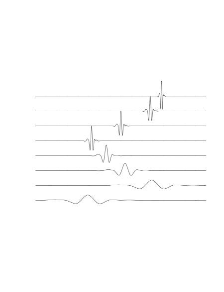
Figure 1: Wavelets at different scales and locations

Let be $f:{\bf R}\longrightarrow{\bf C}$ and the wavelet expansion is

$$f(x)=\sum\limits_{\ell\in{\bf Z}}c_{\ell}\varphi_{\ell}(x)+\sum\limits_{j=0}^{\infty}\sum\limits_{k\in{\bf Z}}c_{jk}\psi_{jk}(x)$$ (10)

If in formulae (10) $c_{jk}=0$ for $j\geq J$, then $f(x)$ has an alternative expansion in terms of dilated scaling functions only $f(x)=\sum_{\ell\in{\bf Z}}c_{J\ell}\varphi_{J\ell}(x)$. This is a finite wavelet expansion, it can be written solely in terms of translated scaling functions. Also we have the shortest possible support: scaling function $DN$ (where $N$ is even integer) will have support $[0,N-1]$ and $N/2$ vanishing moments. There exists $\lambda>0$ such that $DN$ has $\lambda N$ continuous derivatives; for small $N,\lambda\geq 0.55$. To solve our second associated linear problem we need to evaluate derivatives of $f(x)$ in terms of $\varphi(x)$. Let be $\varphi^{n}_{\ell}=\mathrm{d}^{n}\varphi_{\ell}(x)/\mathrm{d}x^{n}$. We consider computation of the wavelet - Galerkin integrals. Let $f^{d}(x)$ be d-derivative of function $f(x)$, then we have $f^{d}(x)=\sum_{\ell}c_{l}\varphi_{\ell}^{d}(x)$, and values $\varphi_{\ell}^{d}(x)$ can be expanded in terms of $\varphi(x)$

$$\phi_{\ell}^{d}(x)=\sum\limits_{m}\lambda_{m}\varphi_{m}(x),$$ (11)

where $\lambda_{m}=\int\varphi_{\ell}^{d}(x)\varphi_{m}(x)\mathrm{d}x$ are wavelet-Galerkin integrals. The coefficients $\lambda_{m}$ are 2-term connection coefficients. In general we need to find $(d_{i}\geq 0)$

$$\Lambda^{d_{1}d_{2}...d_{n}}_{\ell_{1}\ell_{2}...\ell_{n}}=\int\limits_{-\infty}^{\infty}\prod\varphi^{d_{i}}_{\ell_{i}}(x)dx$$ (12)

For Riccati case (sextupole) we need to evaluate two and three connection coefficients

$$\Lambda_{\ell}^{d_{1}d_{2}} = \int^{\infty}_{-\infty}\varphi^{d_{1}}(x)\varphi_{\ell}^{d_{2}}(x)dx,$$ (13)

$$\Lambda^{d_{1}d_{2}d_{3}} = \int\limits_{-\infty}^{\infty}\varphi^{d_{1}}(x)\varphi_{\ell}^{d_{2}}(x)\varphi^{d_{3}}_{m}(x)dx$$

According to CC method [10] we use the next construction. When $N$ in scaling equation is a finite even positive integer the function $\varphi(x)$ has compact support contained in $[0,N-1]$. For a fixed triple $(d_{1},d_{2},d_{3})$ only some $\Lambda_{\ell m}^{d_{1}d_{2}d_{3}}$ are nonzero: $2-N\leq\ell\leq N-2,\quad 2-N\leq m\leq N-2,\quad|\ell-m|\leq N-2$. There are $M=3N^{2}-9N+7$ such pairs $(\ell,m)$. Let $\Lambda^{d_{1}d_{2}d_{3}}$ be an M-vector, whose components are numbers $\Lambda^{d_{1}d_{2}d_{3}}_{\ell m}$. Then we have the first reduced algebraical system : $\Lambda$ satisfy the system of equations $(d=d_{1}+d_{2}+d_{3})$

$$A\Lambda^{d_{1}d_{2}d_{3}} = 2^{1-d}\Lambda^{d_{1}d_{2}d_{3}},$$ (14)

$$A_{\ell,m;q,r} = \sum_{p}a_{p}a_{q-2\ell+p}a_{r-2m+p}.$$

By moment equations we have created a system of $M+d+1$ equations in $M$ unknowns. It has rank $M$ and we can obtain unique solution by combination of LU decomposition and QR algorithm. The second reduced algebraical system gives us the 2-term connection coefficients. For nonquadratic case we have analogously additional linear problems for objects (12). Solving these linear problems we obtain the coefficients of nonlinear algebraical system (6) and after that we obtain the coefficients of wavelet expansion (8). As a result we obtained the explicit time solution of our problem in the base of compactly supported wavelets with the best possible localization in the phase space, which allows us to control contribution from each scale of underlying multiresolution expansions.

In the following parts we consider extension of this approach to the case of (periodic) boundary conditions, the case of presence of arbitrary variable coefficients and more flexible biorthogonal wavelet approach.

We are very grateful to M. Cornacchia (SLAC), W. Herrmannsfeldt (SLAC), Mrs. J. Kono (LBL) and M. Laraneta (UCLA) for their permanent encouragement.

References

- [1] Fedorova, A.N., Zeitlin, M.G. ’Wavelets in Optimization and Approximations’, Math. and Comp. in Simulation, 46, 527-534 (1998).
- [2] Fedorova, A.N., Zeitlin, M.G., ’Wavelet Approach to Polynomial Mechanical Problems’, New Applications of Nonlinear and Chaotic Dynamics in Mechanics, Kluwer, 101-108, 1998.
- [3] Fedorova, A.N., Zeitlin, M.G., ’Wavelet Approach to Mechanical Problems. Symplectic Group, Symplectic Topology and Symplectic Scales’, New Applications of Nonlinear and Chaotic Dynamics in Mechanics, Kluwer, 31-40, 1998.
- [4] Fedorova, A.N., Zeitlin, M.G ’Nonlinear Dynamics of Accelerator via Wavelet Approach’, AIP Conf. Proc., vol. 405, 87-102, 1997, Los Alamos preprint, physics/9710035.
- [5] Fedorova, A.N., Zeitlin, M.G, Parsa, Z., ’Wavelet Approach to Accelerator Problems’, parts 1-3, Proc. PAC97, vol. 2, 1502-1504, 1505-1507, 1508-1510, IEEE, 1998.
- [6] Fedorova, A.N., Zeitlin, M.G, Parsa, Z., ’Nonlinear Effects in Accelerator Physics: from Scale to Scale via Wavelets’, ’Wavelet Approach to Hamiltonian, Chaotic and Quantum Calculations in Accelerator Physics’, Proc. EPAC’98, 930-932, 933-935, Institute of Physics, 1998.
-
[7]
Fedorova, A.N., Zeitlin, M.G., Parsa, Z.,
’Variational Approach in Wavelet Framework to Polynomial
Approximations of Nonlinear Accelerator Problems’,
AIP Conf. Proc., vol. 468, 48-68, 1999.
Los Alamos preprint, physics/9902062. -
[8]
Fedorova, A.N., Zeitlin, M.G., Parsa, Z.,
’Symmetry, Hamiltonian Problems and Wavelets in
Accelerator Physics’,
AIP Conf.Proc., vol. 468, 69-93, 1999.
Los Alamos preprint, physics/9902063. - [9] Dragt, A.J., Lectures on Nonlinear Dynamics, CTP, 1996,
- [10] Latto, A., Resnikoff, H.L. and Tenenbaum E., Aware Technical Report AD910708, 1991.