Oscillatory disintegration of a trans-Alfvénic shock: A magnetohydrodynamic simulation

Abstract

Nonlinear evolution of a trans-Alfvénic shock wave (TASW), at which the flow velocity passes over the Alfvén velocity, is computed in a magnetohydrodynamic approximation. The analytical theory suggests that an infinitesimal perturbation of a TASW results in its disintegration, i.e., finite variation of the flow, or transformation into some other unsteady configuration. In the present paper, this result is confirmed by numerical simulations. It is shown that the disintegration time is close to its minimum value equal to the shock thickness divided by a relative velocity of the emerging secondary structures. The secondary TASW that appears after the disintegration is again unstable with respect to disintegration. When the perturbation has a cyclic nature, the TASW undergoes oscillatory disintegration, during which it repeatedly transforms into another TASW. This process manifests itself as a train of shock and rarefaction waves, which consecutively emerge at one edge of the train and merge at the other edge.

]

I Introduction

It has long been believed that trans-Alfvénic shock waves (TASWs), at which the flow velocity passes over the Alfvén velocity, cannot exist in the real world. Since a stationary trans-Alfvénic shock transition was obtained in a numerical simulation [1], this conventional view point was replaced by an opposite view point. The overall claim was that there is no principal difference between TASWs and fast and slow shocks, at which the flow is super- and sub-Alfvénic, respectively. At the same time, the contradiction inherent in a stationary TASW, which follows from an analytical theory, was not lifted. To reconcile this contradiction, it was suggested that a TASW exists in an unsteady state in which it is repeatedly destroyed and recovered [2]. In the present paper, we show by way of magnetohydrodynamic (MHD) simulation that the evolution of a TASW may have the form of oscillatory disintegration, i.e., reversible transformation into another TASW.

The disintegration of an arbitrary hydrodynamic discontinuity was considered for the first time by Kotchine [3]. After that, Bethe [4] studied the disintegration of shock waves. In the absence of a magnetic field, the shock may disintegrate only in a medium with anomalous thermodynamic properties. The magnetic field enlarges the number of possible discontinuous structures thus giving additional degrees of freedom for the disintegration. The disintegration configurations of arbitrary MHD discontinuities were obtained in Refs. [5]. Furthermore, it has been shown that trans-Alfvénic shock transitions can be realized also through a set of several discontinuities [6], in contrast with fast and slow transitions. However, this fact on its own does not assure that the shock disintegrates.

The important feature that predetermines the disintegration of TASWs is their nonevolutionarity. The problem of evolutionarity was initially formulated for the fronts of combustion [7] and hydrodynamic discontinuities [8]. Evolutionarity is a property of a discontinuous flow to evolve in such a way that the flow variation remains small under the action of a small perturbation. This is not the case for a nonevolutionary discontinuity. At such a discontinuity, the system of boundary conditions, which follow from the conservation laws, does not have the unique solution for the amplitudes of outgoing waves generated by given incident waves. From a mathematical view point this means that the number of unknown parameters (the amplitudes of the outgoing waves and the discontinuity displacement) is incompatible with the number of independent equations. Since a physical problem must have the unique solution, the assumption that the perturbation of a nonevolutionary discontinuity is infinitesimal leads to a contradiction. In fact, the infinitesimal perturbation results in disintegration, i.e., finite variation of the initial flow, or transformation into some other unsteady configuration.

The evolutionarity requirement gives additional restrictions on the flow parameters at a shock, compared to the condition of the entropy increase. The restrictions appear because the direction of wave propagation (toward the discontinuity surface or away from it), and thus the number of the outgoing waves, depends on the flow velocity. If the velocity is large enough then the given wave may be carried down by the flow. Therefore, at an evolutionary discontinuity, the flow velocity must be such that it provides the compatibility of the boundary equations. This form of evolutionarity condition was applied to MHD shock waves in Refs. [9, 10]. As a result, the fast and slow shocks are evolutionary, while the TASWs are nonevolutionary.

This classical picture was challenged when Wu [1] obtained a stationary TASW in a numerical simulation. The existence of a stationary numerical solution does not mean of course that the shock is stable with respect to disintegration or transition into another unsteady flow. Wu [11] demonstrated that a TASW, which is subfast upstream and subslow downstream, disintegrates under the action of a small Alfvén perturbation with a large enough characteristic time. Nevertheless, this numerical result was interpreted as being in a contradiction with the principle of evolutionarity and stimulated the efforts to modify or even disprove this principle.

It was suggested that the free parameters that describe a nonunique structure of a TASW [12] or the amplitudes of strongly damping dissipative waves [13] should be included in the number of unknown parameters when solving the problem of evolutionarity. This would make the TASW evolutionary. In both cases, however, the perturbation is confined within the shock transition layer. Consequently, it does not enter into the boundary conditions, which relate the quantities far enough from the transition layer, and thus it does not contribute to the evolutionarity [14].

Wu [12] also argued that the TASW whose nonevolutionarity is based on separation of Alfvén perturbations from the remaining perturbations [10] becomes evolutionary in the case of a nonplanar shock structure because in this case the separation formally does not take place. However, as shown by Markovskii [14], the coupling of the small-amplitude Alfvén modes with a low enough frequency to the remaining modes is weak (unless the shock is of the type close to one of the degenerate types, Alfvén discontinuity or switch shocks). Therefore the coupling becomes essential only when the small perturbation generates large variation of the flow, which is the same result as predicted by the principle of evolutionarity.

There is one more finding that favors the nonexistence of stationary TASWs. As discussed by Kantrowitz and Petschek [15], the TASWs are isolated solutions of Rankine-Hugoniot problem, which do not have neighboring solutions corresponding to small deviations of boundary conditions. Wu and Kennel [16] introduced a new class of trans-Alfvénic shock-like structures with noncoplanar boundary states. The thickness of such a structure increases in the course of time, and it eventually evolves to a large-amplitude Alfvén wave. It was thus shown that neighboring to a TASW are time-dependent configurations, which are not solutions of the Rankine-Hugoniot problem. In addition, Falle and Komissarov [17] recently considered stationary TASWs of all possible types and showed that the shocks disintegrate if the boundary values deviate from their initial values.

Strictly speaking, a TASW, in contrast with fast and slow shocks, becomes a time-dependent shock-like structure once it is perturbed by a small-amplitude Alfvén wave because the Alfvén wave violates the coplanarity condition. This fact, already on its own, means that the TASW becomes unsteady under the action of the small perturbation. However, the scenario for its evolution depends on the initial configuration and on the nature of the perturbation. After the disintegration, the magnetic field reversal given at the initial nonevolutionary shock may be taken either by a secondary TASW or by an Alfvén discontinuity. Both structures are nonevolutionary [2, 14]. Therefore single disintegration does not lift the contradiction inherent in a TASW. The main question that we solve in this paper is what happens to the post-disintegration nonevolutionary configuration. We show that the secondary TASW is again unstable with respect to disintegration and that the evolution of a TASW may have the form of oscillatory disintegration. In Sec. II, we describe the simulation method. In Sec. III, we discuss the results of the calculations. Our conclusions are presented in Sec. IV.

II Numerical method

We take the MHD equations in the following form

$${\partial\rho\over\partial t}+{\partial\rho v_{x}\over\partial x}=0,$$ (2)

$${\partial\rho v_{x}\over\partial t}+{\partial\over\partial x}\biggl{(}p+\rho v_{x}^{2}+{\textstyle{1\over 2}}{\bf B}_{\perp}^{2}-{\textstyle{4\over 3}}\eta{\partial v_{x}\over\partial x}\biggr{)}=0,$$ (3)

$${\partial\rho{\bf v}_{\perp}\over\partial t}+{\partial\over\partial x}\biggl{(}\rho v_{x}{\bf v}_{\perp}-B_{x}{\bf B}_{\perp}-\eta{\partial{\bf v}_{\perp}\over\partial x}\biggr{)}=0,$$ (4)

$${\partial{\bf B}_{\perp}\over\partial t}+{\partial\over\partial x}\biggl{(}v_{x}{\bf B}_{\perp}-B_{x}{\bf v}_{\perp}-\nu_{m}{\partial{\bf B}_{\perp}\over\partial x}\biggr{)}=0,$$ (5)

$${\partial\over\partial t}\biggl{(}{\textstyle{1\over 2}}\rho v^{2}+{p\over\gamma-1}+{\textstyle{1\over 2}}{\bf B}_{\perp}^{2}\biggr{)}+{\partial\over\partial x}\biggl{[}\rho v_{x}\biggl{(}{\textstyle{1\over 2}}v^{2}$$ (6)

$$\quad+{\gamma\over\gamma-1}{p\over\rho}\biggr{)}+\biggl{(}{\bf B}_{\perp}\cdot\biggl{(}v_{x}{\bf B}_{\perp}-B_{x}{\bf v}_{\perp}-\nu_{m}{\partial{\bf B}_{\perp}\over\partial x}\biggr{)}\biggr{)}$$ (7)

$$\quad-\eta\biggl{(}{\textstyle{4\over 3}}v_{x}{\partial v_{x}\over\partial x}+\biggl{(}{\bf v}_{\perp}\cdot{\partial{\bf v}_{\perp}\over\partial x}\biggr{)}\biggr{)}\biggr{]}=0.$$ (8)

Here the subscript ”$\perp$” denotes the vector component perpendicular to the $x$ axis, $B_{x}={\rm const},$ magnetic diffusivity $\nu_{m}$ and viscosity $\eta$ are put constant and equal to 0.1 in all calculations, and we use the units such that the factor $4\pi$ does not appear. The initial distribution of the MHD quantities is given by the following formulas

$$\rho={\textstyle{1\over 2}}(\rho_{\uparrow}+\rho_{\downarrow})-{\textstyle{1\over 2}}(\rho_{\uparrow}-\rho_{\downarrow}){\rm tanh}({x/L}),$$ (10)

$$v_{x}={\textstyle{1\over 2}}(v_{x\uparrow}+v_{x\downarrow})-{\textstyle{1\over 2}}(v_{x\uparrow}-v_{x\downarrow}){\rm tanh}({x/L}),$$ (11)

$$p={\textstyle{1\over 2}}(p_{\uparrow}+p_{\downarrow})-{\textstyle{1\over 2}}(p_{\uparrow}-p_{\downarrow}){\rm tanh}({x/L}),$$ (12)

$$B_{y}=B_{\tau}{\rm cos}(\theta),\qquad B_{z}=B_{\tau}{\rm sin}(\theta),$$ (13)

$$v_{y}=v_{\tau}{\rm cos}(\theta),\qquad v_{z}=v_{\tau}{\rm sin}(\theta),$$ (14)

$$B_{\tau}= {\textstyle{1\over 2}}(\mid B_{\perp\uparrow}\mid+\mid B_{\perp\downarrow}\mid)$$ (16)

$$-{\textstyle{1\over 2}}(\mid B_{\perp\uparrow}\mid-\mid B_{\perp\downarrow}\mid){\rm tanh}({x/L}),$$

$$v_{\tau}= {\textstyle{1\over 2}}(\mid v_{\perp\uparrow}\mid+\mid v_{\perp\downarrow}\mid)$$ (18)

$$-{\textstyle{1\over 2}}(\mid v_{\perp\uparrow}\mid-\mid v_{\perp\downarrow}\mid){\rm tanh}({x/L}),$$

$$\theta={\textstyle{\pi\over 2}}(1+{\rm tanh}({x/L})),$$ (19)

where the subscripts ”$\uparrow$” and ”$\downarrow$” denote the quantities in the asymptotic upstream and downstream regions, respectively.

After the configuration relaxes to a steady state, it is perturbed by an Alfvén wave specified by the expression

$$B_{z}={\textstyle{1\over 2}}\delta B_{z}\biggl{(}1+{\rm tanh}\biggl{(}{x-x_{0}\over l}\biggr{)}\biggr{)},$$ (21)

$$v_{z}=-B_{z}/\sqrt{\rho}.$$ (22)

This wave moves downstream. The configuration is set by putting $B_{x}=0.89,$ $L=1.45,$ and

$$B_{y\uparrow}=0.93,\qquad B_{y\downarrow}=-0.8,$$ (24)

$$B_{z\uparrow}=v_{z\uparrow}=0.,\qquad B_{z\downarrow}=v_{z\downarrow}=0.,$$ (25)

$$v_{x\uparrow}=1.,\qquad v_{x\downarrow}=0.55042,$$ (26)

$$v_{y\uparrow}=1.04494,\qquad v_{y\downarrow}=-0.49476,$$ (27)

$$\rho_{\uparrow}=1.,\qquad\rho_{\downarrow}=1.81681,$$ (28)

$$p_{\uparrow}=0.00116,\qquad p_{\downarrow}=0.56319.$$ (29)

This corresponds to a ${\rm II\rightarrow III}$ shock, for which $V_{+\uparrow}>v_{x\uparrow}>V_{Ax\uparrow}$ and $V_{Ax\downarrow}>v_{x\downarrow}>V_{-\downarrow},$ where $V_{+}$ and $V_{-}$ are the fast and slow magnetosonic velocities.

We solve Eq. (II) using a uniform grid and an explicit conservative Lax-Wendroff finite-difference scheme with physical dissipation [18]. The time step is limited by the Courant-Friedrichs-Lewy (CFL) condition and by the dissipation timescale. The boundary values are obtained by hyperbolic interpolation. The numerical interval $-50<x<+300$ is covered by 2600 grid points. The interval is chosen in such a way that no large-amplitude wave reaches the boundaries during the computation time. Small-amplitude waves pass through the boundaries without any detectable reflection which could affect the flow inside the simulation region. We have tested our code for a smaller mesh and a corresponding time step determined by the CFL condition as well as for the same mesh and a time step smaller than that determined by the CFL condition. The test showed that there is no considerable dependence of our results on the mesh size and time step.

III Results of simulations

Equation (II) does not exactly describe the shock structure. Therefore the flow undergoes time variations until it adjusts to a stationary shock transition. The resulting boundary values differ slightly from those given by Eq. (22) but the difference is less than 1%. The conservation laws for these new values are fulfilled with the precision less than 0.1%. The stationary configuration is then perturbed by a small-amplitude Alfvén wave with $l=-L,$ $x_{0}=-40,$ and $\delta B_{z}=0.025$ or $\delta B_{z}=-0.025$ (Fig. 1). Note that $\delta B_{z}$ is about 50 times smaller than $\mid{\bf B}_{\uparrow}\mid.$ Although in the case of an upstream incident wave the perturbation of $B_{z}$ and $v_{z}$ (not shown) is carried to the downstream region, the boundary conditions for the Alfvén waves are incompatible. Therefore the given Alfvén perturbation pumps $B_{z}$ and $v_{z}$ into the shock or out of the shock, depending on the sign of $B_{z}$ inside the transition layer. Since $B_{z}$ inside the transition layer is nonzero, the shock behaves in different ways under the action of the perturbations with positive and negative $\delta B_{z}.$ If the shock and the perturbation carry $B_{z}$ of the same sign, the shock disintegrates into a ${\rm II\rightarrow III}$ shock of a smaller amplitude, a large-amplitude slow shock, and some other structures of a much smaller amplitude (Fig. 2a,b).

If the shock and the perturbation carry $B_{z}$ of opposite signs, the situation is somewhat peculiar. The main secondary structures are a TASW and a slow rarefaction (Fig. 3a,b). However, these structures do not become separated. The reason is that the secondary TASW is of a so-called ${\rm II\rightarrow IV=III}$ type [19]. This means that the downstream velocity at the shock is exactly equal to the slow magnetosonic velocity. Therefore there is no disintegration in the usual sense but the configuration becomes unsteady because the right boundary of the slow rarefaction moves away from the TASW, while the left boundary remains attached to the shock. Note that the rarefaction wave is attached to the TASW not at the density peak but somewhere to the right of the peak. This is related to the fact that the density profile of a ${\rm II\rightarrow IV}$ shock has a maximum (see, e.g., Ref. [11]), in contrast with the monotonic profile of a ${\rm II\rightarrow III}$ shock.

From the moment when the Alfvén wave with $\delta B_{z}>0$ arrives to the shock, the disintegration starts almost immediately, in contrast with the result of Wu [11]. The reason is that the disintegration time depends on the shock type and on its initial state. This can be understood as follows. The important characteristic of a TASW, introduced by Kennel et al. [19], is the integral of $B_{z}$ over the transition layer,

$$I_{z}=\int\limits_{x\downarrow}^{x\uparrow}B_{z}dx.$$ (30)

This integral fixes the nonunique structure of a TASW. For a ${\rm II\rightarrow III}$ shock, the quantity $I_{z}$ takes two distinct values, $I_{z0}$ and $-I_{z0},$ and, for a ${\rm I\rightarrow III}$ or ${\rm II\rightarrow IV}$ shock, it falls into the interval $-I_{z0}<I_{z}<I_{z0}.$ The quantity $I_{z0}$ depends on the boundary values, and it tends to infinity when the shock approaches an Alfvén discontinuity or a switch shock, which is intermediate between evolutionary and nonevolutionary shocks. This result was obtained for almost parallel small-amplitude shocks, but one may expect that it remains qualitatively valid in the general case.

When an Alfvén wave is incident on a TASW, it changes $I_{z}.$ If we start from a planar ${\rm I\rightarrow III}$ or ${\rm II\rightarrow IV}$ shock ($I_{z}=0$), as in the case studied by Wu [11], the quantity $\mid I_{z}\mid$ first has to reach the value $I_{z0}.$ Only after that it falls into the forbidden region, and the disintegration starts. In the case of a ${\rm II\rightarrow III}$ shock, there is a different situation. Since $I_{z}$ takes only distinct values $I_{z0}$ and $-I_{z0},$ the disintegration starts immediately, and the disintegration time is close to its minimum value $L/V,$ approximately equal to 30 in our case, where $V$ is a relative velocity of the secondary discontinuities.

Let us now follow the further evolution of the post-disintegration configuration under the action of a small perturbation. Our main conclusion is that the secondary TASW is again unstable with respect to disintegration. At the same time, the way of evolution depends on a form of the perturbation. We first discuss the case where the perturbation of the secondary TASW is such that $I_{z}$ continues to increase or decrease, in particular where the perturbation is equal to its initial positive (Fig. 2b,c) or negative (Fig. 3b,c) value. If the perturbation of $B_{z}$ is positive then the shock spreads in space, with all the jumps, except for $\Delta B_{y}$ and $\Delta v_{y},$ decreasing in time. It thus approaches a large-amplitude Alfvén wave. If the perturbation is negative, the shock first passes through the state in which $I_{z}=0.$ This is not in a contradiction with the analytical theory, because a ${\rm II\rightarrow IV}$ shock may have a planar structure, in contrast with a ${\rm II\rightarrow III}$ shock [19]. When $\mid I_{z}\mid$ reaches a critical value, the shock disintegrates (Fig. 3b), and after that it spreads in space approaching a large-amplitude Alfvén wave (Fig. 3c). The precursor of the disintegration is the peak in $B_{y}$ curve in Fig. IIb.

We now turn to a cyclic perturbation. We impose the perturbation described by Eq. (II) in such a way that $B_{z}$ changes sign at $x=-40$ and the Alfvén wave now carries the perturbation of the same amplitude but opposite sign. After the first disintegration starts (at $t=20$ for $\delta B_{z}>0$ and at $t=670$ for $\delta B_{z}<0$), the opposite sign perturbation arrives to the TASW each 150 units of time. The resulting configuration is such that the increase of $\mid I_{z}\mid$ is repeatedly replaced by its decrease, and the shock undergoes oscillatory disintegration. The disintegration configurations after several cycles are shown in Figs. 4 and 5. As can be seen from the figures, the configuration emits a sequence of contact discontinuities. The contact discontinuities move with the flow velocity, which is approximately equal to that given by Eq. (26). The corresponding time interval between the discontinuities is equal to 150.

Downstream of the TASW, there is a wave train, which consists of slow shock and rarefaction waves. These structures are not standing in the flow. They consecutively emerge at the left edge of the train and merge at the right edge. The merging is seen in Fig. 22b at $x\approx 150.$ We note that, in the case of a negative initial perturbation, the transition through the state with $I_{z}=0$ is not necessary for the oscillatory disintegration to occur. If the perturbation changes sign for the first time before $I_{z}$ becomes negative, the disintegration configuration is similar to that shown in Fig. 30, except for the sign of $I_{z}$ inside the shock.

Finally, the shock comes to a steady state only in a degenerate case where the perturbation of the secondary TASW exactly compensates the nonzero value of $B_{z}$ and $v_{z}$ outside of the transition layer. We emphasize that in all but the degenerate cases the small Alfvén perturbation makes the TASW unsteady, in contrast with fast and slow shocks. However, there remains a question. Formally, the initial TASW becomes a time-dependent structure, much like the secondary TASW, since the Alfvén perturbation arrives to the initial shock. The question is why the initial TASW disintegrates when $I_{z}$ increases monotonically, while the secondary TASW does not. To answer this question, we first mention that the secondary TASW is more close to a finite-amplitude Alfvén wave than the initial shock. Alfvén waves, as well as switch shocks, are singular structures. As shown by Kennel et al. [19], the quantity $dI_{z0}/dq$ tends to infinity as the shock approaches these singular structures. Here $q=B_{y\uparrow}/B_{y\downarrow}$ characterizes the jumps of the boundary values at the shock with a given $I_{z},$ and $I_{z0}(q)$ is an allowed curve in which a ${\rm II\rightarrow III}$ shock has a stationary structure.

Assume now that the initial shock is in the state $I_{z}=I_{z0}(q_{0}).$ A small Alfvén perturbation changes $I_{z}.$ For the shock to remain in the curve $I_{z0}(q),$ a change of $q$ is required. In the general case, the variation of $I_{z}$ is comparable with the variation of $q,$ and thus with the jumps of the boundary values at the TASW. In this case, the evolution has the form of disintegration. By contrast, if the shock is close to the singular structure, the given variation of $I_{z}$ requires a small variation of $q,$ and the jumps of the boundary values are adjusted to $I_{z0}(q)$ in a diffusion-like manner. It should be mentioned that the curves $I_{z0}(q)$ were obtained by Kennel et al. [19] for small-amplitude shocks propagating almost parallel to the magnetic field. Nevertheless, we speculate that, in our simulation, the initial TASW has a small enough $dI_{z0}/dq$ to disintegrate, while for the secondary TASW the quantity $dI_{z0}/dq$ is large enough to dim the disintegration. Such an explanation does not imply that a TASW cannot disintegrate more than one time in principle. Furthermore, in our simulation run with a positive constant $\delta B_{z},$ there is an evidence for a possible second disintegration at $t=380.$ However, the second disintegration is too faint to contend that it indeed takes place.

IV Conclusions

We have performed a numerical simulation of a trans-Alfvénic shock wave. The shock that we have considered is of a ${\rm II\rightarrow III}$ type, i.e., it is subfast upstream and superslow downstream. We have shown that the shock disintegrates under the action of a small Alfvén perturbation. The resulting configuration includes a secondary TASW, a large-amplitude slow shock or rarefaction wave, and other small-amplitude structures. We have also demonstrated that the secondary TASW is again unstable with respect to disintegration. When the perturbation has a cyclic nature, the shock undergoes an oscillatory disintegration. This result is in a qualitative agreement with our previous finding [2]. This process shows up as a train of slow shock and rarefaction waves, which consecutively emerge at one edge of the train and merge at the other edge. At the same time, the disintegration configuration of a small-amplitude almost parallel TASW discussed by Markovskii [2] includes alternating TASWs and Alfvén discontinuities rather than alternating TASWs. This discrepancy is explained by the fact that, in the approximation used in Ref. [2], the difference between the secondary TASW and the Alfvén discontinuity manifests itself in higher orders.

In contrast with the results of Wu [11], the disintegration starts almost immediately after the Alfvén perturbation arrives to the initial shock. The characteristic time of this process is equal to that required for the secondary structures to become separated. The reason for this can be seen as follows. TASWs have a nonunique structure. A ${\rm II\rightarrow IV}$ shock transition studied by Wu [11], as well as a ${\rm I\rightarrow III}$ transition, allows a continuous family of integral curves, while the ${\rm II\rightarrow III}$ shock has two distinct integral curves. For given boundary values, each integral curve is fixed by the definite parameter. The incident Alfvén wave changes the parameter and thus the shock structure. In the case of a ${\rm I\rightarrow III}$ or ${\rm II\rightarrow IV}$ shock, some time passes until the parameter falls into a forbidden region, and only after that the shock disintegrates. In the case of a ${\rm II\rightarrow III}$ shock, its structure immediately becomes inconsistent with the boundary values under the action of the Alfvén wave, which initiates the disintegration.

Thus, our simulations confirm that a TASW becomes unsteady when it is perturbed by a small-amplitude incident wave. Furthermore, an almost vanishing perturbation results in considerable dynamics at relatively small timescales. The scenario for the shock evolution depends on its initial state and on the nature of the perturbation. In particular, the evolution may have the form of oscillatory disintegration in which the shock repeatedly transforms into another TASW.

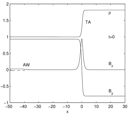
FIG. 1.: Inintial distribution of the density and magnetic field at the TASW perturbed by a small-amplitude Alfvén wave with positive (solid line) and negative (dashed line) value of $\delta B_{z}$.

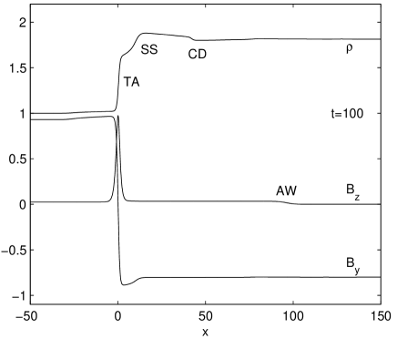
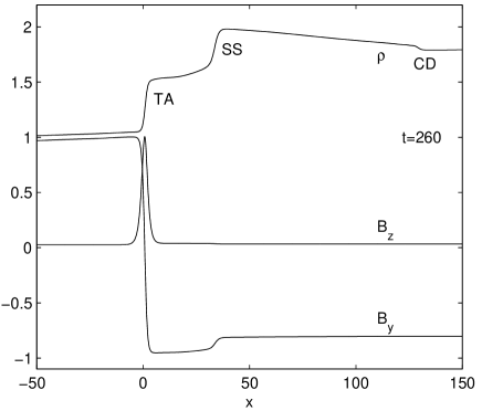
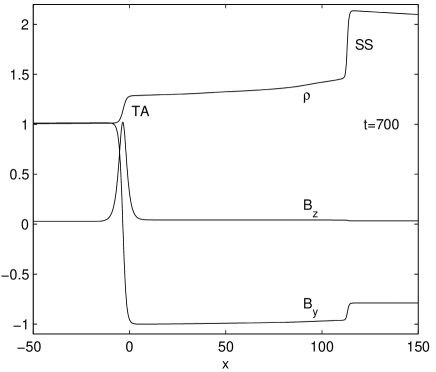
(a) (b) (c)

FIG. 2.: Disintegration configuration for a constant positive perturbation at $t=100$ (a), $t=260$ (b), and $t=700$ (c).

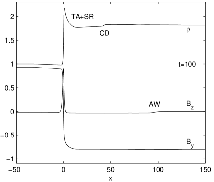
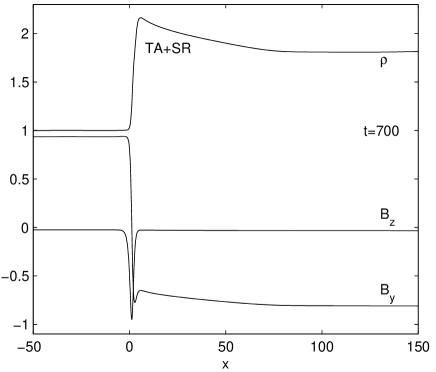
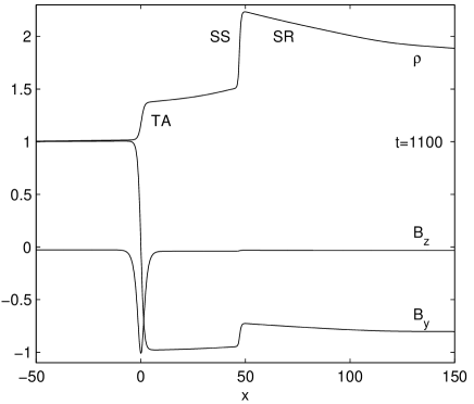
(a) (b) (c)

FIG. 3.: Disintegration configuration for a constant negative perturbation at $t=100$ (a), $t=700$ (b), and $t=1100$ (c).

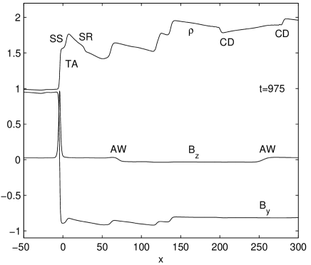
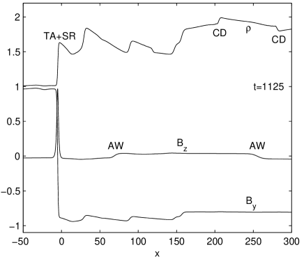
(a) (b) (c)

FIG. 4.: Configuration after several cycles of duration 150 time units at $t=975$ (a), $t=1125$ (b), and $t=1275$ (c). Oscillatory disintegration is started by a positive initial perturbation. The perturbation changes sign for the first time at $t=150.$

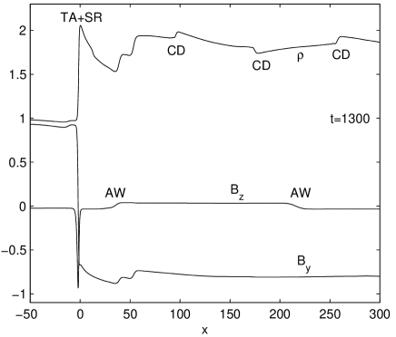
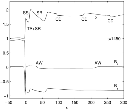
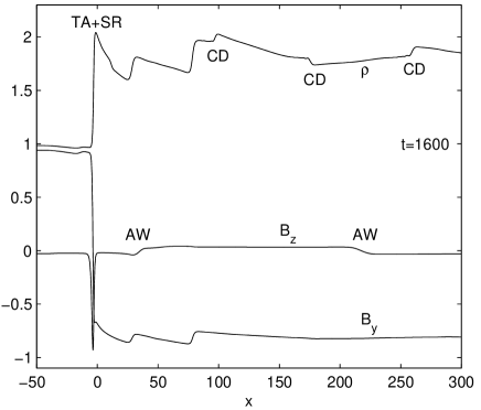
(a) (b) (c)

FIG. 5.: Configuration after several cycles of duration 150 time units at $t=1300$ (a), $t=1450$ (b), and $t=1600$ (c). Oscillatory disintegration is started by a negative initial perturbation. The perturbation changes sign for the first time at $t=800.$