Adaptive walks on time-dependent fitness landscapes

Abstract

The idea of adaptive walks on fitness landscapes as a means of studying evolutionary processes on large time scales is extended to fitness landscapes that are slowly changing over time. The influence of ruggedness and of the amount of static fitness contributions are investigated for model landscapes derived from Kauffman’s $NK$ landscapes. Depending on the amount of static fitness contributions in the landscape, the evolutionary dynamics can be divided into a percolating and a non-percolating phase. In the percolating phase, the walker performs a random walk over the regions of the landscape with high fitness.

Most work on Darwinian evolution so far has been concerned with evolution in constant environments on the one hand (e.g., see [1, 2, 3] for the field of population genetics, or [4] for adaptive walks), and coevolutionary processes on the other hand (e.g., see [5, 6] for ecological models like Lotka-Volterra systems, or [7, 8, 9] for Artificial Life type computer simulations). The case in which a species is subjected to a changing environment, without being able to influence it, has been studied only rarely. Most work of the latter type is considering a single periodically changing optimum [10, 11, 12, 13]. In such situations, the evolutionary dynamics acts as a low pass filter [14]. The optimum can only be tracked if the oscillation frequency is sufficiently low.

In this work, we are considering evolution in high-dimensional fluctuating fitness landscapes, with different amounts of dynamic and static fitness contributions. The motivation of this work comes from in vivo evolution of proteins. Living organisms use a huge amount of different proteins. Where does this diversity originate from? When looking at a single protein in a particular species, the protein appears to be in a local optimum, without any better mutants nearby. However, to account for the observed diversity, there must be mechanisms that allow to move on from one local optimum to another sporadically. The simplest mechanism one can consider is one in which large mutations sometimes carry a protein into a distant region in the genotype space. Although this mechanism cannot completely be rejected, it is unlikely that large mutations play a predominant role in protein evolution. A large mutation is essentially a random jump into the genotype space, leading with extremely high probability to an amino acid sequence that cannot fold correctly anymore. Therefore, large mutations will in almost all cases not produce a viable protein.

A mechanism that works with small mutations is drift on neutral networks. It has been mostly studied for RNA [15, 16, 17], but it can also be considered in the case of proteins [18]. On a neutral network, mutations change the amino acid sequence, but leave the protein fold and, more importantly, the protein’s active region unaltered. From time to time, the drifting sequence comes close to a sequence with higher fitness, and then a transition to a new local optimum takes place. This theory works well for in vitro experiments [19], but it is unclear whether enough neutrality exists in vivo to allow for sufficient drift [20, 21, 22]. There exists evidence that in some cases, no neutral amino acid substitutions exist in living organisms (e.g., for Drosophila m.’s alcohol dehydrogenase locus [23]) and that the environment can select for extremely small fitness differences [24, 25]. The reason why this cannot be observed in in vitro experiments is probably that the experiments are not sensitive enough [25].

Benner and Ellington [20] have suggested a different mechanism that could work with small mutations and in the absence of neutrality. They propose that slow environmental changes generate a constant genetic drift which can be accounted for the protein diversity. This idea has never been studied quantitatively in a mathematical model.

Here, we are going to study a model which demonstrates that indeed a slowly changing environment can generate something like a constant genetic drift. We will call this drift “environmentally guided drift”. It is not a diffusion process, such as neutral drift [1]. The population as a whole moves through the genotype space, since transitions to selectively advantageous states happen very fast, as first order phase transitions [26, 27]. Adaptive walks are particularly suitable to study such phenomena, and we will use them throughout this paper, neglecting population effects or crossover of genotypes.

The statement that the population always remains located in the genotype space, and that hence the dynamics can be approximated with an adaptive walk, can only be justified if the environmental changes are very slow. If this is the case, i.e., if the fitness landscape does change only marginally over time intervals of the length of typical waiting times between two transitions, the adaptive walk approximation should be valid under the same assumptions as in static landscapes. Note that this means, on the other hand, that in our model the adaptive walk must be allowed to do a number of jumps prior to significant changes in the landscape. As a consequence, the walker will often have the chance to reach a local optimum before it starts out for a new peak because of the deforming landscape. Later in this paper, we will discuss the adiabatic limit, which is an even slower time scale. In the adiabatic limit, the changes happen so slowly that for every change in the fitness landscape the adaptive walk can always find a local optimum.

As example landscapes, we choose Kauffman’s $NK$ landscapes [4, 28], which are spin glass-like landscapes commonly used for the study of adaptive walks. Although they cannot be directly related to the true landscapes underlying in vivo protein evolution, their tunable degree of ruggedness makes them a good tool to study general effects in rugged landscapes. In a $NK$ landscape, the fitness of a bit string of length $N$ is defined as the average over each bit’s fitness contribution. The contributions depend on the state of the corresponding bit as well as on the state of $K$ other bits interacting with it. We can write the fitness $f$ as:

$$f=\frac{1}{N}\sum_{i=1}^{N}f_{i}(\{S\}_{i})\,,$$ (1)

where $\{S\}_{i}$ is the state of the $K+1$ bits influencing the fitness contribution of bit $i$. In Kauffman’s original formulation, the functions $f_{i}(\{S\}_{i})$ are realized as tables containing a different quenched random fitness contribution for every state $\{S\}_{i}$. Here we are interested in a time-dependent form of Eq. (1). One possibility has been proposed by Levitan and Kauffman [29], who have studied the case that the fitness cannot be measured exactly. In their work, the measured fitness $f^{\prime}$ equals the true fitness $f$ plus a noise term $g(t)$. Such an approach has proven suitable to study the effects of noise in chemical engineering problems [30]. However, it does not work here, since we are interested in local deformations of the landscape, and not in a global noise-induced shift. What we do instead is to use time-dependent functions $f_{i}(\{S\}_{i},t)$. Note the general difference in the model of Levitan and Kauffman and of ours. In their model, the fitness landscape is static, but can only be measured with finite accuracy. In our model, the fitness landscape itself is changing, but the fitness can be measured exactly. Considering the long time scale we are addressing, we can assume that noise does not play a prominent role here. The single walker represents the mean of a population, as noted above. In the population mean, the noise is averaged out. We will later discuss how the model could be altered for noise too intense to allow that assumption, or for populations so small that destabilizing effects can occur.

We choose the functions $f_{i}(\{S\}_{i},t)$ to be continuous in time. Noisy, discontinuous fitness contributions seem to be unappropriate to model a slowly changing environment. In principle, one could of course add a noise term on top of each fitness contribution, or study landscapes with mixed noisy and continuous contributions, but this is not our objective here.

Not necessarily all fitness contributions need to be truly time dependent. Some may be equal to a constant,

$$f_{i}(\{S\}_{i},t)=C{{}_{i},\{S\}_{i}}\,.$$ (2)

It is useful to keep track of the amount of static contributions in the landscape. We denote the fraction of static contributions by $f_{\rm S}$. Adaptive walks on time-dependent $NK$ landscapes show several distinct classes of behavior, most strongly influenced by $f_{\rm S}$.

So far we have described the basis of our model, now we have to specify the actual form of the fitness contributions. For data analysis, it is useful to impose periodic boundary conditions on the fitness landscape, i.e.,

$$f(t+T)=f(t)\,,$$ (3)

with oscillation period $T$. Throughout the rest of this work, we will stick to this choice. Its advantage rests in the easy comparison of a bit string’s evolution in different oscillation periods. In particular, it allows to use the concept of environmentally linked networks introduced below.

The form of the functions $f_{i}(\{S\}_{i},t)$ can in principle be arbitrarily complicated. We are going to consider a simple trigonometric time dependency,

$$f_{i}(\{S\}_{i},t)=\frac{1}{2}[\sin(\omega_{\{S\}_{i}}t+\delta_{\{S\}_{i}})+1]\,.$$ (4)

This introduces only a single additional constant per fitness contribution, if compared to the static landscape. The frequencies $\omega_{\{S\}_{i}}$ and the phases $\delta_{\{S\}_{i}}$ are chosen randomly when constructing the landscape, and are then kept fixed for all times $t$. The phases are distributed uniformly in the interval $[0;2\pi)$ so that the resulting fitness landscape is homogeneous in time. We set the frequencies to $\omega_{\{S\}_{i}}=2\pi n_{\{S\}_{i}}/T$, with $n_{\{S\}_{i}}$ being integral, and $T$ being arbitrary, but the same for all $\omega_{\{S\}_{i}}$, to obtain a periodic fitness landscape with oscillation period $T$. If we want a fitness contribution to be constant, we set the corresponding frequency $\omega_{\{S\}_{i}}$ to 0.

We have done a large number of simulations with different choices for $N$ and $K$, with different sets of oscillation frequencies, and also with more complicated functions $f_{i}(\{S\}_{i},t)$, in which the oscillations have additional random amplitudes and offsets. In all cases, the basic patterns are very similar. The parameters having the strongest influence on the observed behavior are the ruggedness $K$ and the fraction of static fitness contributions $f_{\rm S}$. In Figs. 1-3, some typical runs of adaptive walks in oscillating $NK$-landscapes are presented. In the simulations leading to these plots, we used $N=20$ and $K=8$. Additionally, we employed only a single oscillation mode. This means, all frequencies $\omega_{\{S\}_{i}}$ were either set to zero or set to some fixed value $\omega=2\pi/T$. The oscillation period $T$ was set to $T=1000$, which can be considered large in a system with $N=20$. A local optimum can typically be found in about 100 time steps in a static $NK$ landscape with such $N$. The adaptive walk was performed exactly as in Kauffman’s original work: a random point mutation was accepted if it increased the bit string’s fitness. Otherwise, the mutation was rejected.

Figure 1 shows an example of the evolutionary dynamics with a relatively low fraction of static fitness contributions. The resulting pattern is a chaotically changing fitness. With almost every accepted mutation, a new genotype is encountered. The environmental changes constantly lead the walker into regions previously not visited. This reminds one of a random walk. However, there are some differences between the adaptive walk and a random walk. We will discuss them below.

The behavior of the adaptive walk changes drastically with increasing $f_{\rm S}$. The higher amount of static fitness contributions reduces the number of possible advantageous mutations in every time step. The bits connected to static contributions freeze out in a locally optimal state, and only the sites connected to oscillating contributions can still change. Hence, the dynamics gets confined in a small region of the genotype space. The same mutational patterns are seen over and over again in the different oscillation periods. In the fitness plots, we can identify this behavior with a periodic or almost periodic change of the fitness, as shown in Fig. 2. Using the language of dynamic systems, we can say that the attractor of an adaptive walk on an oscillating landscape with intermediate $f_{\rm S}$ is a noisy limit cycle. With some small probability $p$, the process can leave a limit cycle. Several transitions between such metastable limit cycles are shown in Fig. 3. The mean fitness can increase or decrease because of the transitions. The frequency with which transitions occur depends on the actual value of $f_{\rm S}$. The larger $f_{\rm S}$, the rarer can transitions be observed.

These metastable states remind one very much of the metastability induced by finite populations on static landscapes with a high degree of neutrality [31, 32, 33], however they are generated through a completely different mechanisms. A slight qualitative difference between the two types of metastability is that here, the transitions lead regularly to a decrease of a metastable state’s average fitness, whereas in neutrality-induced transitions, this is mostly not the case. Nevertheless, the work of Nimwegen et al. shows that with very small populations, the evolutionary dynamics on a landscape with neutrality can as well display transitions leading to a decrease of fitness [32]. The interesting point of our findings here is that we find metastability under the complete absence of neutrality.

Let us now address the question whether the transitions actually lead to an increase in fitness, or whether advantageous and disadvantageous transitions balance each other. In Fig. 4, we show the expected fitness as a function of time for 100 oscillations with a period of $T=2560$. The expected fitness was obtained by averaging over 50 independent runs. We have chosen $f_{\rm S}=0.6$, which is well in the metastable regime. We observe that the most important fitness gain is reached during the first couple of oscillations (the curve starts of from $\langle f\rangle=0.5$ for $t=0$). Nonetheless, for the complete duration of the 100 oscillations, we observe a constant slight increase in the fitness. A linear fit to the expected fitness from time step $10^{4}$ to the end of the recording gives an increase in fitness of $1.03\times 10^{-4}$ per oscillation period. Ultimately, for much longer simulation runs, the expected fitness reaches an asymptotic value. Note that the slight fitness increase over many oscillation periods is an effect peculiar to the metastable regime. In the chaotic regime the expected fitness reaches its asymptotic value very quickly, after a few oscillation periods.

The adaptive walk’s efficiency to find regions of high fitness can be judged from the mean fitness encountered during the walk. Figure 5 shows the mean fitness, averaged over several independent adaptive walks, as a function of the oscillation period $T$. The curve corresponding to the chaotic regime, with $f_{\rm S}=0$, starts off at a mean fitness of 0.5 for small $T$. This is the average fitness on the landscape, and hence the walker approximately does a random walk on the landscape. For larger $T$, the mean fitness quickly grows and reaches a value close to the average of a local optimum in the landscape. Although the movement in the genotype space appears to be chaotic, the expected fitness of the walker at any point in time is as large as the expected highest fitness an adaptive walk in a comparable static landscape would encounter. Therefore, for large $T$ the walker’s movement can be considered as a random walk confined to the regions of high fitness in the genotype space. When we increase the amount of static contributions in the landscape, the average fitness is above 0.5 even for very fast environmental changes. For larger $T$, the average fitness increases towards the average height of local optima in the landscape, and even significantly above it. The latter occurs in time-dependent landscapes as long as only a tiny amount of time-dependent contributions is present. To understand why this happens, consider a bit string in which all but one bit have only static contributions. The remaining bit may also give a static contribution if it is set to 0, and a time-dependent one if it is set to 1. For the times when the time-dependent contribution is smaller than the static one, the bit will be set to 0, and otherwise it will be set to 1. This effectively increases the average height of local optima in dynamic landscapes. The effect is most pronounced if the number of static contributions is moderately large, for $f_{\rm S}$ around 0.8.

At this point, it is interesting to ask what proportion of the genotype space can actually be reached through environmentally guided drift. The question can be addressed with the concept of environmentally linked networks (EL networks). We define an EL network to be the set of all points in the genotype space the adaptive walk can reach at times $nT$, $n=0,1,2,\dots$, starting from a fixed position in the genotype space. We will say an EL network percolates if it consists of infinitely many points. This definition is similar to the usual definition of the percolating cluster on the Bethe lattice, and is the appropriate way to define percolation in high-dimensional spaces [34]. It can be applied literally only in the limit $N\rightarrow\infty$. However, the genotype space grows so fast with increasing $N$ that this restriction can be neglected.

If the walker is for small $f_{\rm S}$ indeed doing a random walk over the landscape, or over the landscape’s regions of high fitness, as we supposed above, then we should find a percolating EL network in the chaotic regime.

The study of EL networks in oscillating $NK$ landscapes is computationally very demanding, since we have to go through the full oscillation periods in the simulation. Hence, we have to restrict ourselves to moderate $T$ and $N$. In the examples below, we have again used $\omega_{i}=\omega=2\pi/T$ with $T=1000$, as well as $N=20$.

Figure 6 shows the fraction $\gamma$ of new genotypes among all the genotypes encountered at the beginning of each oscillation period. This is a measure for the size of an EL network. A value near 1 means a new genotype has been encountered in almost every oscillation period. On the other hand, a value near 0 means the network’s size is small, thus confining the adaptive walk in a limited region of the genotype space. In the limit of infinitely many oscillation periods, only percolating networks can have a positive $\gamma$, whereas finite networks yield $\gamma=0$. Therefore, $\gamma$ is a proper order parameter indicating a percolation transition. Clearly, in numerical experiments the number of oscillation periods over which the measurement is taken is finite, and therefore we will observe a positive $\gamma$ even in the non-percolating regime. In the case of Fig. 6, the value $\gamma$ was obtained from averaging over 60 adaptive walks, each on a different fitness landscape. Every adaptive walk endured 200 oscillation periods. The error bars present the standard deviations of the single measurements.

Let us begin the discussion of Fig. 6 with the graph on the right, for $K=8$. We find a $\gamma$ close to 1 for small $f_{\rm S}$, and a vanishing $\gamma$ for $f_{\rm S}\approx 1$. The standard deviations are very small in both limiting regimes. In the region about $f_{\rm S}\approx 0.5$, a sharp drop in $\gamma$ can be observed, accompanied with an enormous increase in the error bars. This is good evidence for the existence of a percolation transition with critical point $f_{\rm S}^{\ast}$ around 0.5. The large error bars are a sign for critical fluctuations, observed in 2nd order phase transitions. The graph on the left of Fig. 6, for $K=2$, shows a very different behavior. The quantity $\gamma$ does not reach higher than about 0.2, and the error bars are large for the whole range of $f_{\rm S}$. We do not see a clear percolation transition for this much less rugged landscape. The large error bars indicate that the finite $\gamma$ for small $f_{\rm S}$ is rather an artifact due to the finite sampling than a true result. We have done comparable simulations for the range of $K$ from 0 up to 14, and what we generally observe is that the transition becomes sharper with increasing $K$.

We can understand the above observation in the adiabatic limit. For the case of a Fujiyama landscape ($K=0$), the EL network degenerates to a single point in this limit, and percolation can consequently not be observed. On the other hand, the completely random landscape we obtain for $K=N-1$ presents a multitude of local optima, and the changes in the landscape provide the opportunity to hop from one local optimum to another in a random fashion during the oscillation periods. The landscapes with intermediate $K$ interpolate between the two extremes. This argument shows that ruggedness must generally promote the movement in the genotype space for the low-$f_{\rm S}$ regime, a situation completely opposite to the case of static landscapes, where ruggedness is regarded as an impediment to the movement in the genotype space. If the changes happen on a slow enough time scale, the increased mobility does not lead to an error catastrophe through which all information is lost, such as the breakdown of the quasispecies for large mutation rates [35]. As we saw in Fig. 5, the fitness is constantly in the region of average local optima. We observe this also in the example run displayed in Fig. 1. The fitness is chaotically changing, but it is always well above the landscape mean of 0.5. An error catastrophe occurs only if the environmental changes happen very fast compared to the typical adaptation time of the system.

So far, we disregarded noise or loss of information because of very small populations in our model. Both have the effect to enable the acceptance of mutations leading to lower fitness. Here, we could incorporate them by adding noise to the fitness as in [29], or by accepting bad mutations with some probability. As long as these mechanisms do not lead to an error catastrophe on a static landscape, they should not very much alter the dynamics on a slowly changing landscape from what we have found here.

Evolution in a slowly changing environment follows a dynamics very different from the situation in a fixed environment. The environmentally guided drift drives genes out of local optima, and drags them around in the genotype space. We have presented evidence for the existence of a giant EL network for $f_{\rm S}$ below some critical $f_{\rm S}^{*}$ in landscapes with sufficient ruggedness. Consequently, in this regime the whole genotype space can be transversed by means of environmentally guided drift. The guided drift can provide – in absence of any neutral pathways in the fitness landscape – an efficient mechanism to generate constantly new genotypes, albeit at every single point in time the system seems to be trapped in a local optimum. We could show that the efficiency of the environmentally guided drift is related to the ruggedness of the landscape. A more rugged landscape provides more opportunities to move around under environmental changes than a landscape with only a few peaks. Consequently, the rugged landscapes observed in protein evolution [20] can promote protein evolution in an ever changing environment, instead of hindering it. If we have a population that decomposes into several subpopulations not coupled with each other through selection, these subpopulations will disperse and move to completely different regions of the genotype space because of environmentally guided drift, even if the process starts off from a completely homogeneous population and if all individuals in the system feel the same environmental changes at the same time. The decoupling of the subpopulations can occur, for example, if the population lives in a very large geographical territory, so that individuals living in one part do not directly interact with individuals living in another part, or if a physical barrier forms at one point in time that divides the territory into several independent regions. As a consequence, rugged landscapes combined with slow environmental changes should inevitably lead to a large variety of different evolutionary solutions for the same problems.

Although the EL networks used here for data analysis are only meaningful in periodic landscapes, the conclusions drawn from their study should also hold in non-periodic situations. The reason why environmentally guided drift becomes so efficient for small $f_{\rm S}$ is that constantly new local optima appear nearby. Therfore, if the changes are non-periodic, but the landscape has sufficient ruggedness, the adaptive walk should similarly behave like a random walk over the landscape’s regions of high fitness.

An effect tightly connected to the periodicity of the landscape, on the other hand, is the appearance of limit cycles. The dynamics in oscillating $NK$ landscapes is above the percolation transition dominated by noisy limit cycles, with sporadically occuring transitions from one limit cycle to another. The system goes through several noisy limit cycles until a stable limit cycle, or a stable fixed point, is reached. This effect reminds one of the behavior of evolution on landscapes with a high degree of neutrality. There, evolution proceeds on neutral networks, with sporadic transitions between them, until a stable local optimum is reached.

The model studied in the present paper, i.e., an adaptive walk on an oscillating $NK$-landscape, is certainly too simplistic to be accounted for as a realistic model of the in vivo evolution of proteins in a changing environment. In particular, it can be argued whether sinusoidally changing fitness contributions are justified. Nevertheless, such simple models often capture the qualitative properties of more realistic situations. Similar percolation transitions can probably be found also in other time-dependent landscapes with sufficient ruggedness.

In future work, it should be interesting to study the percolation transition in more detail, and to determine for what $K$ a percolating regime actually exists. Furthermore, the interplay between static and dynamic fitness contributions should also be investigated in other fitness landscapes.

FIG. 1.: The evolutionary dynamics is chaotic for small $f_{\rm S}$.

FIG. 2.: With increasing $f_{\rm S}$, some bits in the bit string freeze out, and the evolutionary pattern becomes more and more oscillatory.

FIG. 3.: The oscillatory states are metastable, and transitions between them can occur.

FIG. 4.: Average fitness over time in adaptive walks over a landscape with $f_{\rm S}=0.6$. The dashed line indicates the result of a least squares fit. The exact slope is $m=4.00824\times 10^{-8}\pm 2.057\times 10^{-10}$.

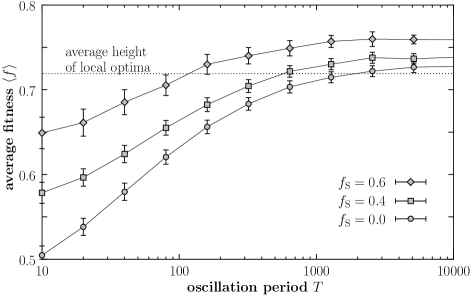
FIG. 5.: Mean fitness encountered during an adaptive walk as a function of the oscillation period $T$. The fitness was averaged over 50 independent adaptive walks, of which each endured 100 oscillation periods.

FIG. 6.: Fraction of newly encountered genotypes $\gamma$ at the beginning of each oscillation period in oscillating fitness landscapes. The quantity $\gamma$ was averaged over 60 independent adaptive walks, of which each endured 200 oscillations with period $T=1000$.

- [1] M. Kimura, The neutral theory of molecular evolution (Cambridge University Press, Cambridge, MA, 1984).
- [2] W. J. Ewens, Mathematical Population Genetics (Springer-Verlag, New York, 1979).
- [3] J. S. Gale, Theoretical Population Genetics (Unwin Hyman, London, 1990).
- [4] S. A. Kauffman, The Origins of Order (Oxford University Press, Oxford, 1992).
- [5] H. I. Freedman, Deterministic Mathematical Models in Population Ecology (Marcel Dekker, New York, 1980).
- [6] Mathematical Ecology. An Introduction, edited by T. G. Hallam and S. A. Levin (Springer-Verlag, New York, 1986).
- [7] W. D. Hillis, in Artificial Life II, edited by C. G. Langton, C. Taylor, J. D. Farmer, and S. Rasmussen (Addison-Wesley, Reading, MA, 1991), pp. 313–324.
- [8] S. A. Kauffman and S. Johnsen, J. theor. Biol. 149, 467 (1991).
- [9] C. W. Reynolds, in Artificial Life IV, edited by R. A. Brooks and P. Maes (MIT Press, Cambridge, MA, 1994), pp. 59–69.
- [10] B. Charlesworth, Genet. Res. (Camb) 61, 205 (1993).
- [11] R. Lande and S. Shannon, Evolution 50, 434 (1996).
- [12] K. Ishii, H. Matsuda, Y. Iwasa, and A. Sasaki, Genetics 121, 163 (1989).
- [13] T. Bäck, in Proceedings of the 1998 IEEE International Conference on Evolutionary Computation (IEEE Press, Piscataway, NJ, 1998), pp. 446–451.
- [14] A. J. Hirst and J. E. Rowe, J. theor. Biol. (1998), submitted.
- [15] C. V. Forst, C. Reidys, and J. Weber, in Advances in Artificial Life, Vol. 929 of Lecture Notes in Artificial Intelligence, ECAL ’95, edited by F. Morán, A. Moreno, J. Merelo, and P. Chacón (Springer, Berlin, Heidelberg, New York, 1995), pp. 128–147, SFI Preprint 95-10-094.
- [16] M. A. Huynen, P. F. Stadler, and W. Fontana, Proc. Natl. Acad. Sci. USA 93, 397 (1996).
- [17] C. Reidys, P. F. Stadler, and P. Schuster, Bull. Math. Biol. 59, 339 (1997), SFI Preprint 95-07-058.
- [18] A. Babajide, I. L. Hofacker, M. J. Sippl, and P. F. Stadler, Folding & Design 2, 261 (1997), SFI Preprint 96-12-085.
- [19] C. V. Forst, J. Biotechnology 64, 101 (1998).
- [20] S. Benner and A. D. Ellington, CRC Critical Reviews in Biochemistry 23, 369 (1988).
- [21] M. Kreitman and H. Akashi, Annu. Rev. Ecol. Syst. 26, 403 (1995).
- [22] M. Kreitman, Bioessays 18, 678 (1996).
- [23] M. Kreitman, Nature 304, 412 (1983).
- [24] A. Berry and M. Kreitman, Genetics 134, 869 (1993).
- [25] J. W. Thatcher, J. M. Shaw, and W. J. Dickinson, Proc. Natl. Acad. Sci. USA 95, 253 (1998).
- [26] J. H. Gillespie, The American Naturalist 121, 691 (1983).
- [27] C. Adami, Introduction to Artificial Life (Telos, Springer-Verlag Publishers, Santa Clara, 1998).
- [28] S. A. Kauffman and E. D. Weinberger, J. theor. Biol. 141, 211 (1989).
- [29] B. Levitan and S. Kauffman, Molecular Diversity 1, 53 (1995).
- [30] B. Levitan, in Annual Reports in Combinatorial Chemistry and Molecular Diversity, edited by M. R. Pavia, W. H. Moos, A. D. Ellington, and B. K. Kay (ESCOM Publishers, The Netherlands, 1997), Vol. 1, pp. 95–152.
- [31] E. van Nimwegen, J. P. Crutchfield, and M. Mitchell, Physics Letters A 229, 144 (1997).
- [32] E. van Nimwegen, J. P. Crutchfield, and M. Mitchell, Theoretical Computer Science, to appear, SFI working paper 97-04-035.
- [33] J. P. Crutchfield and E. van Nimwegen, in Evolution as Computation, Lecture Notes in Computer Science, edited by L. F. Landweber, E. Winfree, R. Lipton, and S. Freeland (Springer-Verlag, New York, 1999).
- [34] D. Stauffer and A. Aharony, Introduction to Percolation Theory, 2nd ed. (Taylor & Francis, Basingstoke Hauts, UK, 1992).
- [35] M. Eigen, J. McCaskill, and P. Schuster, Adv. Chem. Phys. 75, 149 (1989).