Considerations on the Diffraction Limitations to the Spatial Resolution of Optical Transition Radiation

X.Artru^a, R.Chehab^b, K.Honkavaara^b,c,∗, A.Variola^b,d

^a Institut de Physique Nucléaire de Lyon IN2P3-CNRS and Université Claude Bernard, F-69622 Villeurbanne Cedex, France
^b Laboratoire de l’Accélérateur Linéaire IN2P3-CNRS, Université de Paris-Sud, B.P.34, F-91898 Orsay Cedex, France
^c Helsinki Institute of Physics, P.O.Box 9, FIN-00014 University of Helsinki, Finland
^d presently at CERN

^∗ Corresponding author. Fax.+33 1 69071499, e-mail: khonkava@lalcls.in2p3.fr

Abstract

The interest in using optical transition radiation (OTR) in high energy (multiGeV) beam diagnostics has motivated theoretical and experimental investigations on the limitations brought by diffraction on the attainable resolution. This paper presents calculations of the diffraction effects in an optical set-up using OTR. The OTR diffraction pattern in a telescopic system is calculated taking into account the radial polarization of OTR. The obtained diffraction pattern is compared to the patterns obtained by other authors and the effects of different parameters on the shape and on the size of the OTR diffraction pattern are studied. The major role played by the radial polarization on the shape of the diffraction pattern is outlined. An alternative method to calculate the OTR diffraction pattern is also sketched.

Keywords: optical transition radiation, spatial resolution, diffraction, polarization

1 Introduction

Optical transition radiation (OTR) provides an attractive method for diagnostics of charged particle beams and it has been used for instance for electron beam diagnostics in the keV-MeV energy region. There have been, however, statements that the geometrical resolution of OTR might deteriorate drastically at high energies due to the diffraction phenomenon [1]. During the last years there have been several studies concerning the resolution of OTR (see Refs.[2] - [11]) and this paper extends these investigations concentrating in the optical diffraction of OTR in a telescopic system.

In order to study the resolution of the optical transition radiation, we shall calculate the diffraction pattern of OTR on the image plane of a telescope, which is situated in the direction of specular reflection of the incident particle (i.e. only the case of backward OTR is considered). Naturally, the results are valid on the image plane of any kind of imaging system. Scalar diffraction theory (see, for example, Ref.[12] or Ref.[13]) used by D.W.Rule and R.B.Fiorito in Refs.[3]-[5] does not take into account the polarization of the field. Precisely, in the case of OTR the polarization is important, since the polarization of OTR is not uniform, but radial (the electric field is in a plane containing the wave vector and the direction of the specular reflection). This can be taken into account by considering separately the horizontal and the vertical field components. The method is similar to that used by A.Hofmann and F.Méot in Ref.[14] for synchrotron radiation. Our treatment yields a satisfactory description of the diffraction phenomenon and provides a relatively simple, clear and straightforward method to compute the transition radiation diffraction pattern.

After recalling some basic characteristics of the optical transition radiation and of the scalar diffraction theory we shall consider the diffraction effects of diaphragms in a telescope and use the obtained expression in the particular case of OTR. The diffraction pattern of OTR will thus allow us to study the influence of different parameters on its shape and size. Our result will also be compared with others using the same hypothesis (polarized character of OTR) [9], [11]. A comparison of the OTR diffraction pattern with the well known standard diffraction pattern and with the ”scalar” diffraction pattern similar to that obtained by D.W.Rule and R.B.Fiorito [3]-[5] will be presented. As OTR is radially polarized, a comparison with isotropic radiation, radially polarized, will allow us to precise the respective contribution of the non-constant angular distribution of OTR. A more theoretical treatment will also be given for the OTR diffraction.

2 Recalls

Before calculating the diffraction pattern of OTR in a telescopic system, we shall recall some basic characteristics of OTR and of the scalar diffraction theory.

2.1 Optical transition radiation

Transition radiation is emitted when a charged particle crosses a boundary between two media of different optical properties. The emission occurs both into the forward and backward hemispheres with respect to the separating surface. Here, we shall consider the case of a single boundary between a metal and vacuum. Due to metal opacity, only forward (resp. backward) OTR is observed when the electron moves from metal to vacuum (resp. vacuum to metal). If the surface is perfectly reflecting ($r=r_{\parallel}=r_{\perp}=-1$), the angular distribution is approximately given (in Gaussian units) by (see, for example, Ref.[15]):

$$I(\theta)=\frac{\mathrm{d}^{2}W}{\mathrm{d}\omega\mathrm{d}\Omega}=\frac{e^{2}}{\pi^{2}c}\left(\frac{\theta}{\gamma^{-2}+\theta^{2}}\right)^{2}$$ (1)

where $\theta$ is the angle with respect to the electron velocity (forward OTR) or to the direction of the specular reflection of that velocity (backward OTR). $\gamma$ is the Lorentz factor of the electron, and Eq.(1) is valid for $\gamma\gg 1$ and $\theta\ll 1$. From now on we will consider the case of backward OTR (Fig.1).

The emitted electric field has two polarization components: one in the plane of observation ($\hat{z}_{s}\hat{n}$ -plane in Fig.1) and the other one in the plane perpendicular to that. In the transverse plane perpendicular to the direction of specular reflection ($\hat{x}\hat{y}$ -plane in Fig.1), the electric field is radially polarized and in that plane it can be decomposed into horizontal ($\hat{x}$-direction) and vertical ($\hat{y}$-direction) components.

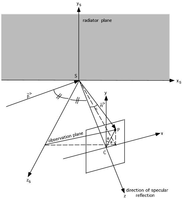
Figure 1: Definition of coordinates and planes.

2.2 Transformation of image fields by an optical system in the scalar wave diffraction theory

Let us first consider a wave of frequency $\omega=(c/n)k$ propagating between two planes $\Pi$ and $\Pi^{\prime}$ without any lenses between them. In the scalar wave theory, with the approximation of Gaussian optics, the amplitude $\psi(P^{\prime})$ in the plane $\Pi^{\prime}$ is related to the amplitude $\psi_{0}(P)$ in the plane $\Pi$ by

$$\psi(P^{\prime})=-\frac{i}{\lambda}\int_{\Pi}\psi_{0}(P)\frac{e^{ikR}}{R}\mathrm{d}S$$ (2)

where $R$ is the distance between points $P$ and $P^{\prime}$. The time-dependent factor $e^{-i\omega t}$ has been factored out both in $\psi$ and $\psi_{0}$. We can treat the ($1/R$)-factor as a constant (in the Gaussian optics approximation) and write

$$\psi(P^{\prime})=A\int_{\Pi}\psi_{0}(P)e^{ikR}\mathrm{d}S$$ (3)

where $A=i/(\lambda L)$ and $L$ is the distance between the two planes.

Let us now consider the case where one or several ”non-diaphragmed” lenses are inserted between the planes $\Pi$ and $\Pi^{\prime}$. By ”non-diaphragmed” lens, we mean a lens with an aperture much larger than the transverse size of the optical wave packet. Eq.(3) can be generalized as 

$$\psi(P^{\prime})=A\int_{\Pi}\psi_{0}(P)e^{ik\mathcal{L}(P,P^{\prime})}\mathrm{d}S$$ (4)

where $\mathcal{L}(P,P^{\prime})$ is the optical distance between points $P$ and $P^{\prime}$, i.e. the integral

$$\mathcal{L}(P,P^{\prime})=\int_{P}^{P^{\prime}}n\mathrm{d}l$$ (5)

along the geometrical optical ray connecting $P$ and $P^{\prime}$; $n$ is the refractive index. $A$ is a complex factor, which depends only on the location of the planes and which we will not calculate, since we are interested only in the shape of the OTR image.

3 Diffraction effect of diaphragms in a telescope

In this chapter we consider diffraction effect caused by the diaphragms of a telescope, and in the next one we will take into account also the special properties of optical transition radiation.

We have taken the experimental set-up used in our experiment at Orsay [6] as the geometrical basis for the diffraction calculations. In this experiment backward optical transition radiation emitted by a 2 GeV electron beam was measured in the direction of the specular reflection. The set-up consisted of an OTR radiator, two lenses in a telescopic configuration and a CCD-camera; henceforth the CCD is referred to as a screen. The first lens had a focal length of 1 m and a diameter of 8 cm; the focal length of the second one was 25 cm and the diameter 14 cm. The first lens with a smaller diameter gives the effective aperture limitation of the system. The telescope geometry is presented in Fig.2.

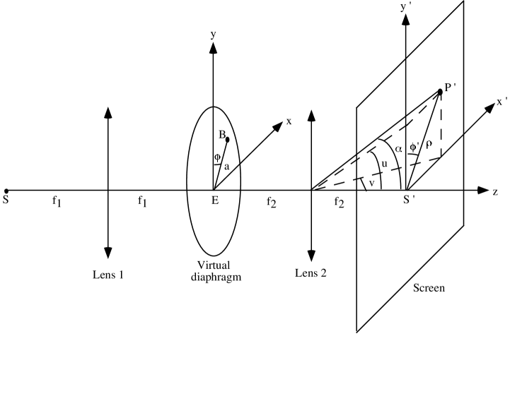
Figure 2: Schematic set-up.

We will treat the effect of the real diaphragm (at the first lens) in a slightly approximate but convenient way, replacing this diaphragm by a virtual one, with the same diameter, but located in the common focal plane between the lenses . In that plane, the spatial coordinates are directly related to the angles of the emitted radiation ($a=f_{1}\theta$).

Our observation point $P^{\prime}$ is situated in the image plane of the telescope (see Fig.2) and, according to Eq.(4), the modulus of the field at this point is related to the amplitude $\psi_{0}$ in the common focal plane by

$$|\psi(P^{\prime})|=A|\int_{\epsilon}\psi_{0}(B)e^{ik\mathcal{L}(B,P^{\prime})}\mathrm{d}\epsilon|$$ (6)

where $A$ is a normalization factor. The integration is performed over the aperture area $\epsilon$ of the virtual diaphragm.

The coordinates of a point $B$ in the virtual diaphragm are $x=a\sin\phi$ and $y=a\cos\phi$ (Fig.2). In the image plane we use ”prime” coordinates: $x^{\prime}=\rho\sin\phi^{\prime}$ and $y^{\prime}=\rho\cos\phi^{\prime}$. The angular directions $v$ and $u$ in the small angle approximation can be written as

$$v = \frac{x^{\prime}}{f_{2}}=\frac{\rho}{f_{2}}\sin\phi^{\prime}=\alpha\sin\phi^{\prime}$$ (7)

$$u = \frac{y^{\prime}}{f_{2}}=\frac{\rho}{f_{2}}\cos\phi^{\prime}=\alpha\cos\phi^{\prime}$$ (8)

In the phase factor of Eq.(6) we are interested in the relative phase difference. All the rays leaving the diaphragm in a particular direction are focused by the second lens into the same point of the screen (see Fig.3).

Figure 3: Sketch of rays after the virtual diaphragm.

According to the theorem of Malus [16], all the rays perpendicular to a given surface ($BF$ in Fig.3) have an equal optical path length from the surface to the focus point (point $P^{\prime}$ in Fig.3), and thus the optical path difference between the rays $EAP^{\prime}$ and $BDP^{\prime}$ is $d=|EF|$. This distance is the projection of the vector $\overrightarrow{EB}$ onto the direction of vector $\overrightarrow{EA}$ : $d=|\overrightarrow{EB}\cdot(\overrightarrow{EA}/|\overrightarrow{EA}|)|=vx+uy$, where $x$ and $y$ are the coordinates of point $B$ and $v$ and $u$ are the angular directions given by Eq.(7) and Eq.(8), respectively. The corresponding phase difference can now be written as $\delta=-kd=-k(vx+uy)$. In polar coordinates the last parenthesis can be written as

$$vx+uy=\frac{x^{\prime}}{f_{2}}x+\frac{y^{\prime}}{f_{2}}y=\frac{\rho}{f_{2}}a\cos(\phi-\phi^{\prime})$$ (9)

Since OTR is symmetrical about the $z$ -axis, there is no preferred value of the angle $\phi^{\prime}$, and we can select $\phi^{\prime}=0$ and write the modulus of the diffracted amplitude in the point $P^{\prime}$ on the screen as

$$|\psi(P^{\prime})|=A|\int_{0}^{2\pi}\int_{0}^{a_{0}}\psi_{0}(a,\phi)\mathrm{exp}(-i\frac{2\pi}{\lambda}\frac{\rho}{f_{2}}a\cos\phi)a\mathrm{d}a\mathrm{d}\phi|$$ (10)

where $k=2\pi/\lambda$ and $\psi_{0}(a,\phi)$ is the amplitude of the wave in the intermediate focal plane. The integration is made in polar coordinates and $a_{0}$ is the radius of the smaller lens (the limiting aperture of the system). It should be noticed that Eq.(10) is a particular form of a two-dimensional Fourier transform of the wave amplitude $\psi_{0}$. We can therefore say, in agreement with Ref.[17, Chap.5,§5.2.2], that the field in the image focal plane of the lens $L_{2}$ is proportional to the Fourier transform of the field in the object focal plane of $L_{2}$. In our derivation, this property appears essentially as a consequence of the Malus theorem.

4 Diffraction of OTR in the telescope

In the calculation of the diffraction pattern of optical transition radiation (i.e. the OTR spot in the image plane of the telescope) we need to consider both the amplitude and the polarization of the incident wave.

The scalar diffraction theory can be used without modification for the vector case if the direction of the field is the same in each point on the diaphragm. The electric field of transition radiation is, however, radially polarized i.e. for every azimuthal angle $\phi$ the field vector has a different direction (it is always pointing to the centre of symmetry). We may take this characteristic into account by considering separately the horizontal and vertical field components. The total intensity is the sum of the intensities from these two components.

When we decompose transition radiation into plane waves with directions of $\theta$, the amplitude is proportional to $\vec{\theta}/(\gamma^{-2}+\theta^{2})$, where $\vec{\theta}$ is a two-dimensional vector. When considering the two polarization components separately, $\vec{\theta}$ can be replaced by ($\theta\sin\phi$) for the horizontal and by ($\theta\cos\phi$) for the vertical component  (Fig.1). The phase of these plane waves is precisely zero in the impact point $S$.

A plane wave, whose direction of propagation has an angle $\theta$ with respect to the direction of specular reflection and whose azimuthal angle is $\phi$, is focused to the point $B=(a,\phi)$ on the virtual diaphragm (where $\theta=a/f_{1}$) and the modulus of the electric field amplitude in this point is given by

$$|E_{\omega}(B)|=C^{\prime}\frac{(a/f_{1})}{\gamma^{-2}+(a/f_{1})^{2}}$$ (11)

where $f_{1}$ is the focal length of the first lens and $C^{\prime}$ is a constant that takes into account the normalization and units.

When considering horizontal and vertical components separately, $|E_{\omega}(B)|$ has to be multiplied by the factor ($\sin\phi$) or ($\cos\phi$), respectively, and we can write

$$\psi_{0h}(a,\phi) = |E_{\omega}(B)|\sin\phi$$ (12)

$$\psi_{0v}(a,\phi) = |E_{\omega}(B)|\cos\phi$$ (13)

where $\psi_{0h}(a,\phi)$ refers to the horizontal component and $\psi_{0v}(a,\phi)$ to the vertical one. We should multiply Eq.(12) and Eq.(13) by a phase factor corresponding to the propagation between $S$ and $B$. However, because $E$ and $B$ are on the same wave surface, the optical paths $SE$ and $SB$ are equal (invoking the Malus theorem), and if we forget the constant phase factor, we do not have any extra phase factors to add into Eq.(12) and Eq.(13).

The total intensity at the point $P^{\prime}$ is the sum of the intensities from the horizontal and the vertical components:

$$I(P^{\prime})=|\mathcal{E}(P^{\prime})|^{2}=|\mathcal{E}(P^{\prime})|_{h}^{2}+|\mathcal{E}(P^{\prime})|_{v}^{2}$$ (14)

In the case of OTR in a telescope, $|\mathcal{E}(P^{\prime})|_{h}$ and $\mathcal{E}(P^{\prime})|_{v}$ are obtained by substituting Eq.(12) and Eq.(13) into Eq.(10). By using the expression given by Eq.(11), we obtain

$$|\mathcal{E}(P^{\prime})|_{h} = A^{\prime}|\int_{0}^{a_{0}}\int_{0}^{2\pi}\frac{(a/f_{1})\sin\phi}{\gamma^{-2}+(a/f_{1})^{2}}\mathrm{exp}(-i\frac{2\pi}{\lambda}\frac{\rho}{f_{2}}a\cos\phi)a\mathrm{d}a\mathrm{d}\phi|$$ (15)

$$|\mathcal{E}(P^{\prime})|_{v} = A^{\prime}|\int_{0}^{a_{0}}\int_{0}^{2\pi}\frac{(a/f_{1})\cos\phi}{\gamma^{-2}+(a/f_{1})^{2}}\mathrm{exp}(-i\frac{2\pi}{\lambda}\frac{\rho}{f_{2}}a\cos\phi)a\mathrm{d}a\mathrm{d}\phi|$$ (16)

where $A^{\prime}$ is a normalization constant.

The integration over $\phi$ in the horizontal component gives zero, thus only the vertical component contributes to the total intensity, and we obtain

$$I(P^{\prime})=|\mathcal{E}(P^{\prime})|_{v}^{2}=C|\int_{0}^{a_{0}}\frac{a^{2}}{\gamma^{-2}+(a/f_{1})^{2}}J_{1}(\frac{2\pi}{\lambda}\frac{\rho}{f_{2}}a)\mathrm{d}a|^{2}$$ (17)

where $J_{1}$ is the first order Bessel function and $C$ a generic normalization constant.

We have defined the angle $\phi$ with respect to the vertical axis. Of course this angle can as well be defined with respect to the horizontal axis. In that case the $\sin\phi$ and $\cos\phi$ -factors in Eq.(12) and Eq.(13) are changed with each other and the horizontal component instead of the vertical one gives the contribution to the intensity of Eq.(17).

The integration over $a$ in Eq.(17) can be performed numerically and the result as a function of the radius $\rho$ on the screen is shown in Fig.4 for our experimental conditions ($E=2$ GeV, $f_{1}=1$ m, $f_{2}=25$ cm, $a_{0}=4$ cm, $\theta_{1}=a_{0}/f_{1}=40$ mrad, $\lambda=500$ nm). This distribution, which represents the diffraction pattern of an OTR source taking into account the radial polarization, is shown around the symmetry axis. Since we are not interested in the absolute intensity, the peak intensity is normalized to unity. The magnification of the used telescope is $M=f_{2}/f_{1}=0.25$; if we use an imaging system with magnification of one, the diffraction pattern is naturally four times wider. The FWHM size of the pattern in Fig.4 is about 4.5 $\mu$m (FWHM $\approx 18$ $\mu$m, when $M=1$). This pattern shape is in full agreement with that of V.A.Lebedev obtained in Ref.[9]. Similar observations concerning this pattern shape are presented in Ref.[10] and Ref.[11].

Figure 4: OTR diffraction pattern (intensity) around the symmetry axis on the image plane of a telescope with magnification $M=0.25$ ($E=2$ GeV, $f_{1}=1$ m, $f_{2}=25$ cm, $M=f_{2}/f_{1}=0.25$, $a_{0}=4$ cm, $\theta_{1}=a_{0}/f_{1}=40$ mrad, $\lambda=500$ nm). In a one-to-one imaging system the size of the diffraction pattern is four times larger.

4.1 Effects of different parameters on the OTR diffraction pattern

Next we study the effects of different parameters on the OTR diffraction pattern. Since we are only interested in the size of the pattern, the peak intensities are always scaled to unity. In all the figures the magnification of the system is 0.25; when using a one-to-one imaging system, the patterns are four times wider.

Fig.5 shows the OTR diffraction pattern for different wavelengths. We can see, as expected, that the size of the pattern scales proportionally to the wavelength. The resolution can be improved when using smaller wavelengths, but if we are out of the optical range ($\lambda{\lower 2.15277pt\hbox{$\stackrel{{\scriptstyle<}}{{\sim}}$}}350$ nm), we can not use an optical imaging system and the experimental conditions become more complicated.

Figure 5: OTR diffraction pattern for different wavelengths ( a) $\lambda=100$ nm, b) $\lambda=500$ nm and c) $\lambda=1$ $\mu$m) on the image plane of a telescope with magnification $M=0.25$. The used parameters are the same as in Fig.4.

In Fig.6 the geometrical size of the aperture ($a_{0}$) is varied. Naturally, the decrease of the aperture size causes an enlargement of the diffraction pattern.

Figure 6: OTR diffraction pattern for different geometrical aperture sizes(a) $a_{0}=10$ cm, b) $a_{0}=4$ cm and c) $a_{0}=1$ cm) on the image plane of a telescope with magnification $M=0.25$. The used parameters are the same as in Fig.4.

Fig.7 shows OTR diffraction pattern for different energies in the GeV energy range. The FWHM size of the distribution is independent of $\gamma$. The difference is in the tails: the higher is the energy, the stronger are the tails.

Figure 7: OTR diffraction pattern for different energies (a) $E=2$ GeV, b) $E=5$ GeV, c) $E=10$ GeV and d) $E=20$ GeV) on the image plane of a telescope with magnification $M=0.25$. The used parameters are the same as in Fig.4.

In Refs.[2],[6],[18] and more recently also in Refs.[10] and [11], it has been considered a possibility to use a mask  to improve the spatial resolution. The effect of a mask can be taken into account by introducing into Eq.(17) an extra pupil function representing the cut caused by the mask. It amounts to set the lower limit of integration in Eq.(17) to $a_{m}$ instead of zero, where

$a_{m}$ is the radius of the mask . A mask reduces the tails, as can be seen in Fig.8, where OTR diffraction pattern for $E=10$ GeV (M=0.25) has been plotted with and without a mask ($a_{mask}=2$ mm). However, it does not affect significantly the FWHM size of the pattern.

Figure 8: Effect of a mask with a radius $a_{m}=2$ mm ($a_{m}/a_{0}=0.05$). $E=\break 10$ GeV; the used parameters are the same as in Fig.4.

4.2 Diffraction of a gaussian emitter

So far, we have considered OTR emitted by a single electron. Diffraction of OTR emitted by a gaussian beam can be treated by convoluting on the image plane the OTR diffraction pattern and a gaussian distribution, which is the image of the beam distribution. In a general form, this is a two-dimensional convolution:

$$I_{\mathrm{conv}}(x,y)=\int\int I(x-x_{1},y-y_{1})\mathcal{O}(x_{1},y_{1})\mathrm{d}x_{1}\mathrm{d}y_{1}$$ (18)

where $I(x,y)$ is the OTR diffraction pattern (Eq.(17)) in cartesian coordinates ($\rho=\sqrt{x^{2}+y^{2}}$) and $\mathcal{O}(x,y)$ the image of the beam profile:

$$\mathcal{O}(x,y)=\frac{1}{\sqrt{2\pi}\sigma_{ix}}\mathrm{exp}(-\frac{x^{2}}{2\sigma_{ix}^{2}})\frac{1}{\sqrt{2\pi}\sigma_{iy}}\mathrm{exp}(-\frac{y^{2}}{2\sigma_{iy}^{2}})$$ (19)

where $\sigma_{ix}$ and $\sigma_{iy}$ are the horizontal and vertical rms sizes of the gaussian beam image.

5 Comparison with standard diffraction

Let us calculate for comparison the diffraction pattern of an ideal isotropic point source (the standard diffraction pattern) in a telescope. In that case $\psi_{0}(a,\phi)={\rm constant}$. By substituting this into Eq.(10) and squaring, we obtain

$$I(P^{\prime})=\mathrm{const}*|\int_{0}^{2\pi}\int_{0}^{a_{0}}\mathrm{exp}(-i\frac{2\pi}{\lambda}\frac{\rho}{f_{2}}a\cos\phi)a\mathrm{d}a\mathrm{d}\phi|^{2}$$ (20)

Integration over $\phi$ and $a$ gives

$$I(P^{\prime})=C|\frac{J_{1}\left(\frac{2\pi}{\lambda}\frac{\rho}{f_{2}}a_{0}\right)}{\left(\frac{2\pi}{\lambda}\frac{\rho}{f_{2}}a_{0}\right)}|^{2}$$ (21)

where $J_{1}$ is the first order Bessel function and $C$ is a generic normalization constant.

In Fig.9 the standard diffraction pattern given by Eq.(21) (curve a) is compared with the OTR diffraction pattern given by Eq.(17) (curve c) in our experimental conditions. The peak intensities are both normalized to unity. We can see that the OTR diffraction pattern is wider (the FWHM size is about 2.7 times that of the standard diffraction pattern) and has a zero in the center.

6 Diffraction of ”scalar OTR”

If we do not take into account the radial polarization of OTR, but only the angular distribution of it, we can use the right hand side of Eq.(11) as the algebraic amplitude. By substituting it into Eq.(10) we obtain

$$|\mathcal{E}(P^{\prime})|=A^{\prime}|\int_{0}^{2\pi}\int_{0}^{a_{0}}\frac{(a/f_{1})}{\gamma^{-2}+(a/f_{1})^{2}}\mathrm{exp}(-i\frac{2\pi}{\lambda}\frac{\rho}{f_{2}}a\cos\phi)a\mathrm{d}a\mathrm{d}\phi|$$ (22)

After integrating over $\phi$ we have

$$I(P^{\prime})=|\mathcal{E}(P^{\prime})|^{2}=C|\int_{0}^{a_{0}}\frac{a^{2}}{\gamma^{-2}+(a/f_{1})^{2}}J_{0}\left(\frac{2\pi}{\lambda}\frac{\rho}{f_{2}}a\right)\mathrm{d}a|^{2}$$ (23)

where $J_{0}$ is the zero order Bessel function and $C$ is a generic normalization constant.

The integration over $a$ can again be performed numerically and the resulting diffraction pattern is plotted in Fig.9 (curve b). The peak intensity is again normalized to unity. This pattern is similar to the pattern obtained by D.W.Rule and R.B.Fiorito in Refs.[3]-[5]. The FWHM size of this ”scalar OTR” diffraction pattern is by a factor $\sim$ 1.2 wider than the FWHM size of the standard diffraction pattern; the FWHM size of the ”vector OTR” pattern given by Eq.(17) is by a factor of $\sim$ 2.2 wider than the FWHM size of the ”scalar” one (Eq.(23)).

Figure 9: Standard diffraction pattern given by Eq.(21) (curve a), ”vector” OTR diffraction pattern given by Eq.(17) (curve c) and ”scalar” OTR diffraction pattern given by Eq.(23) (curve b) on the image plane of a telescope with magnification $M=0.25$. The used parameters are the same as in Fig.4.

7 Importance of the radial polarization in the diffraction phenomenon

For a field which is invariant by rotation about the direction of the specular reflection, the amplitude distribution and the polarization of the field can be described by separate functions $\mathcal{A}$ and $\mathcal{F}$, respectively. According to Eq.(10) we can write

$$|\mathcal{E}(P^{\prime})|_{i}=A|\int_{0}^{2\pi}\int_{0}^{a_{0}}\mathcal{A}(a)\mathcal{F}_{i}(\phi)\mathrm{exp}(-i\frac{2\pi}{\lambda}\frac{\rho}{f_{2}}a\cos\phi)a\mathrm{d}a\mathrm{d}\phi|$$ (24)

where index $i$ refers to the horizontal or to the vertical component. The total intensity is the sum of the intensities from different components: $I(P^{\prime})=\sum_{i}|\mathcal{E}(P^{\prime})|_{i}^{2}$

When the field is radially polarized, the polarization function is $\mathcal{F}_{h}(\phi)=\sin\phi$ for the horizontal component and $\mathcal{F}_{v}(\phi)=\cos\phi$ for the vertical one. The angle $\phi$ is again defined with respect to the vertical axis. Let us consider a hypothetical case in which the field is constant in the amplitude : $\mathcal{A}(a)=\mathrm{constant}$. By substituting these into Eq.(24), we obtain

$$|\mathcal{E}(P^{\prime})|_{h} = \mathrm{const}*|\int_{0}^{2\pi}\int_{0}^{a_{0}}\sin\phi\mathrm{exp}(-i\frac{2\pi}{\lambda}\frac{\rho}{f_{2}}a\cos\phi)a\mathrm{d}a\mathrm{d}\phi|$$ (25)

$$|\mathcal{E}(P^{\prime})|_{v} = \mathrm{const}*|\int_{0}^{2\pi}\int_{0}^{a_{0}}\cos\phi\mathrm{exp}(-i\frac{2\pi}{\lambda}\frac{\rho}{f_{2}}a\cos\phi)a\mathrm{d}a\mathrm{d}\phi|$$ (26)

The integration over $\phi$ in the horizontal component gives again zero and we obtain for the total intensity

$$I(P^{\prime})=|\mathcal{E}(P^{\prime})|_{v}^{2}=C|\int_{0}^{a_{0}}aJ_{1}\left(\frac{2\pi}{\lambda}\frac{\rho}{f_{2}}a\right)da|^{2}$$ (27)

where $C$ is a generic normalization constant.

Eq.(27) is plotted in Fig.10 (curve a) together with the OTR diffraction pattern (curve b). The peak intensities are both normalized to unity. It is important to understand that the peculiar shape of the OTR diffraction pattern in the central region with a zero in the center is essentially determined by the radial polarization. The non-constant angular distribution of OTR only widens the pattern a little: the FWHM value is wider by a factor of $\sim$ 1.2, when the OTR angular distribution is taken into account.

Figure 10: Diffraction pattern on the image plane of a telescope with magnification M=0.25 given by radial polarization: a) isotropic angular distribution (Eq.(27)) and b) OTR angular distribution (Eq.(17)). The used parameters are the same as in Fig.4.

8 Another treatment of OTR diffraction

Diffraction of OTR can also be studied from a more theoretical point of view. A detailed treatment of this kind is presented elsewhere [10] and here we only shortly show that we can obtain, using this method, the same expression for diffraction pattern as obtained in paragraph 4.

The angular distribution of transition radiation in natural units ($c=\hbar=\epsilon_{0}=1$, $e^{2}/4\pi=\alpha=1/137$) can be written as

$$I(\omega,\theta)=\frac{\mathrm{d}^{2}I}{\mathrm{d}\omega\mathrm{d}\Omega}=\omega\frac{\mathrm{d}N}{\mathrm{d}\omega\mathrm{d}\Omega}\simeq\frac{\alpha}{\pi^{2}}\left(\frac{\theta}{\gamma^{-2}+\theta^{2}}\right)^{2}$$ (28)

In the case of forward radiation Eq.(28) is the spectrum emitted by a suddenly accelerated electron and in the backward case the spectrum emitted by a suddenly stopped ”image positron”. The radiation field (in the far-field region) can be decomposed in plane waves

$$\mathbf{E}(t,\mathbf{\vec{r}})=\int\frac{\mathrm{d}^{3}\mathbf{\vec{k}}}{(2\pi)^{3}}\mathbf{\tilde{E}}(\mathbf{\vec{k}})e^{i\mathbf{\vec{k}}\cdot\mathbf{\vec{r}}-i|\mathbf{\vec{k}}|t}$$ (29)

with

$$\mathbf{\tilde{E}}(\mathbf{\vec{k}})\simeq ie\frac{\mathbf{\vec{q}}}{\mathbf{\vec{q}}^{2}+\gamma^{-2}k_{L}^{2}}$$ (30)

where $\mathbf{\vec{q}}$ and $\mathbf{\vec{k_{L}}}$ are the transverse and the longitudinal components of the wave vector $\mathbf{\vec{k}}$, respectively.

The impact parameter profile  is related to the $\mathbf{\vec{q}}$ -Fourier transform of $\mathbf{\tilde{E}}$:

$$I(b) \equiv \frac{\omega}{\mathrm{d}\omega}\frac{\mathrm{d}N}{\mathrm{d}^{2}\mathbf{\vec{b}}}\simeq\frac{1}{\pi}|\mathbf{E}(\omega,\mathbf{\vec{b}}|^{2}$$ (31)

$$= 4\alpha|\int\frac{\mathrm{d}^{2}\mathbf{\vec{q}}}{(2\pi)^{2}}\frac{\mathbf{\vec{q}}}{\mathbf{\vec{q}}^{2}+q_{0}^{2}}f(q)e^{i\mathbf{\vec{q}}\cdot\mathbf{\vec{b}}}|^{2}$$

where $f(q)$ is a cut-off function:

$$f(q)=\Theta(q-q_{m})\Theta(q_{1}-q)$$ (32)

The parameters $q_{0}$, $q_{1}$ and $q_{m}$ are defined as

$$q_{0} = \gamma^{-1}k_{L}\simeq\gamma^{-1}\omega$$ (33)

$$q_{1} = \theta_{1}\omega$$ (34)

$$q_{m} = \theta_{m}\omega$$ (35)

where $\theta_{1}$ is the upper cut-off angle determined by some diaphragm and $\theta_{m}$ the lower cut-off angle determined by some mask. If no mask is used, $\theta_{m}=0\rightarrow q_{m}=0$.

Using the properties of Bessel functions Eq.(31) can be developed as

$$I(b) = 4\alpha|\int\int\frac{\mathrm{d}^{2}\mathbf{\vec{q}}}{(2\pi)^{2}}\frac{\mathbf{\vec{q}}}{\mathbf{\vec{q}}^{2}+q_{0}^{2}}f(q)e^{i\mathbf{\vec{q}}\cdot\mathbf{\vec{b}}}|^{2}$$ (36)

$$= 4\alpha|\mathbf{\vec{\nabla}_{\vec{b}}}\int\int\frac{\mathrm{d}^{2}\mathbf{\vec{q}}}{(2\pi)^{2}}\frac{f(q)}{\mathbf{\vec{q}}^{2}+q_{0}^{2}}e^{i\mathbf{\vec{q}}\cdot\mathbf{\vec{b}}}|^{2}$$

$$= \frac{\alpha}{\pi^{2}}|\mathbf{\vec{\nabla}_{\vec{b}}}\int q\mathrm{d}q\frac{f(q)}{q^{2}+q_{0}^{2}}J_{0}(qb)|^{2}$$

$$= \frac{\alpha}{\pi^{2}}|\int q^{2}\mathrm{d}q\frac{f(q)}{q^{2}+q_{0}^{2}}J_{1}(qb)|^{2}$$

If we substitute for $f(q)$ the sharp cut-off function Eq.(32), we obtain

$$I(b)=\frac{\alpha}{\pi^{2}}|\int_{q_{m}}^{q_{1}}\frac{q^{2}}{q^{2}+q_{0}^{2}}J_{1}(qb)\mathrm{d}q|^{2}$$ (37)

This can be written using the angle $\theta=q\lambda\raise 1.72218pt\hbox{\kern-5.0pt\hbox{--}}\$ and $q_{0}=\gamma^{-1}\lambda\raise 1.72218pt\hbox{\kern-5.0pt\hbox{--}}\ ^{-1}$ (in natural units $\omega=\lambda\raise 1.72218pt\hbox{\kern-5.0pt\hbox{--}}\ ^{-1}$) as

$$I(b)=C_{1}|\int_{\theta_{m}}^{\theta_{1}}\frac{\theta^{2}}{\theta^{2}+\gamma^{-2}}J_{1}\left(\frac{\theta}{\lambda\raise 1.72218pt\hbox{\kern-5.0pt\hbox{--}}\ }b\right)\mathrm{d}\theta|^{2}$$ (38)

If we rewrite the diffraction pattern given by Eq.(17) using $a=f_{1}\theta$, $M$ = magnification = $f_{2}/f_{1}$ and the integration limits $\theta_{1}=a_{0}/f_{1}$ and $\theta_{m}=a_{m}/f_{1}$ (i.e. we have a mask), we obtain

$$I(\rho)=C_{2}|\int_{\theta_{m}}^{\theta_{1}}\frac{\theta^{2}}{\gamma^{-2}+\theta^{2}}J_{1}\left(\frac{2\pi}{\lambda}\frac{\theta}{M}\rho\right)\mathrm{d}\theta|^{2}$$ (39)

We can see that this is identical (excluding the constant factor) to Eq.(38) taking into account the image magnification $\rho=Mb$.

9 Summary and conclusions

In this paper, we have considered the limitations brought by the diffraction to the resolution of OTR images of high energy charged particles. Starting from the scalar wave theory, some basic formulas concerning the wave propagation in an optical system were recalled. Choosing, for the optical system, a telescope which exhibits very simple and interesting properties, we have calculated the diffraction pattern of the OTR wave emitted by one electron. A virtual diaphragm, located in the common focal plane between the lenses of the telescope, allowed us to express the diffraction in a rather simple way. The radial polarization of OTR was taken into account by considering the horizontal and vertical field components separately.

Our result coincides with that of V.A.Lebedev [9] and it is in qualitative agreement with that of D.W.Rule and R.B.Fiorito obtained in the scalar wave approximation [3]-[5]. The obtained diffraction pattern was also compared to the well known standard diffraction pattern. The FWHM size of the OTR diffraction pattern is by factor of $\sim$ 2.2 wider than the ”scalar OTR” pattern and by factor of $\sim$ 2.7 than the standard diffraction pattern.

Consideration of the general shape of the OTR diffraction pattern shows that the FWHM width is insensitive for the particle energy, whereas the tails increase with the energy. These tails may be seen by very sensitive detectors: in that case, a central optical mask constitutes an effective cure.

In conclusion, up to energies considered ($\gamma\sim 5*10^{4}$), the effects of the diffraction, evaluated by the FWHM of the OTR diffraction pattern, are not limiting the resolution. The resolution depends more likely on the properties of the experimental set-up, the contrast sensitivity of the detector and the data treatment procedure.

References

- [1] K.T. Mc Donald, D.P. Russell, ”Methods of Emittance Measurement”, Proceedings of Joint US-CERN School on Observation, Diagnosis and Correction in Particle Beams, October 20-26 1988, Capri, Italy.
- [2] E.W. Jenkins, ”Optical Transition Radiation from a Thin Carbon Foil – A Beam Profile Monitor for the SLC”, Single Pass Collider Memo CN-260 (1983).
- [3] D.W. Rule, R.B. Fiorito, ”Imaging Micron Sized Beams with Optical Transition Radiation”, A.I.P. Conference Proceedings No.229 (1991) p.315.
- [4] D.W. Rule, R.B.Fiorito, ”Beam Profiling with Optical Transition Radiation”, Proceedings of 1993 Particle Accelerator Conference, May 1993, Washington DC, p.2453.
- [5] D.W. Rule, R.B. Fiorito, 1993 Faraday Cup Award Invited Paper, Proceedings of Beam Instrumentation Workshop, Conf. Proc. No. 319 (1994) p.21.
- [6] X. Artru et al., Nucl. Inst. Meth. A410 (1998) 148.
- [7] J.-C. Denard et al., ”High Power Beam Profile Monitor with Optical Transition Radiation”, Proceedings of 1997 Particle Accelerator Conference, June 1997, Vancouver.
- [8] D. Giove et al., ”Optical Transition Radiation Diagnostics”, Proceedings of DIPAC 97, October 1997, Frascati, LNF-97/048(IR), p.251.
- [9] V.A. Lebedev, Nucl. Inst. Meth. A372 (1996) 344.
- [10] X. Artru et al., ”Resolution Power of Optical Transition Radiation: Theoretical Considerations”, Proceedings of RREPS’97, September 1997, Tomsk, Nucl. Inst. Meth. B145 (1998) 160.
- [11] M. Castellano and V.A. Verzilov, ”Spatial Resolution in Optical Transition Radiation (OTR) Beam Diagnostics”, LNF-98/017(P), to appear in Phys.ReV.ST Accel.Beams.
- [12] M. Born and E. Wolf, Principles of Optics, Third (revised) edition, Pergamon Press, 1965.
- [13] L.D. Landau and E.M. Lifshitz, The Classical Theory of Fields, Revised second edition, Pergamon Press, 1962.
- [14] A. Hofmann and F. Méot, Nucl. Inst. Meth. 203 (1982) 483.
- [15] L. Wartski, Thése de doctorat d’Etat, Un. Paris-Sud (1976).
- [16] W.T. Welford, Geometrical Optics, Optical Instrumentation, Vol.1, North-Holland, 1962.
- [17] J.W. Goodman, Introduction to Fourier Optics, McGraw-Hill, 1996.
- [18] S.D. Borovkov et al., Nucl. Inst. Meth. A294 (1990) 101.