Statistical properties of spike trains: universal and stimulus-dependent aspects

Abstract

Statistical properties of spike trains measured from a sensory neuron in-vivo are studied experimentally and theoretically. Experiments are performed on an identified neuron in the visual system of the blowfly. It is shown that the spike trains exhibit universal behavior over short time, modulated by a stimulus-dependent envelope over long time. A model of the neuron as a nonlinear oscillator driven by noise and an external stimulus, is suggested to account for these results. The model enables a theoretic distinction of the effects of internal neuronal properties from effects of external stimulus properties, and their identification in the measured spike trains. The universal regime is characterized by one dimensionless parameter, representing the internal degree of irregularity, which is determined both by the sensitivity of the neuron and by the properties of the noise. The envelope is related in a simple way to properties of the input stimulus as seen through nonlinearity of the neural response. Explicit formulas are derived for different statistical properties in both the universal and the stimulus-dependent regimes. These formulas are in very good agreement with the data in both regimes.

I Introduction

Many cells in the nervous system respond to stimulation by generating action potentials (spikes). Time sequences of these spikes are the basis for encoding information and for communication between neurons [1]. A pattern of spikes across time contains, in addition to the message being encoded, the signature of the biophysical spike generation mechanism, and of the noise in the neuron and its environment [2]. These factors are generally inter-related in a complicated way, and it is not clear how to disentangle their effect on the measured spike train.

The biophysical mechanism for generating action potentials was first described successfully by Hodgkin and Huxley [3]. Their description accounted for the stereotyped shape of an action potential, which is a robust property, largely independent of external conditions. The Hodgkin Huxley model describes the neuron as a complex dynamical system; sustained firing (a continuous train of spikes) comes about when the dynamical system is driven into an oscillatory mode. This picture is consistent with experiments on isolated neurons: many of these tend to fire periodic spike trains in response to direct current injection, implying an oscillator like behavior. The frequency of these trains is deterministically related to the strength of the applied current; Adrian (1928) suggested long ago that this property could be used to code the strength of the input. Different neurons vary in the shape of the response function relating frequency to input. Following Hodgkin and Huxley, many microscopic models of the neuron were constructed in the same spirit [2]. One aim of this type of modeling is to produce the different frequency-current ($f/I$) response curves by fitting model parameters.

Spike trains measured in vivo, however, show a very different behavior: many neurons seem to fire stochastically, even when external conditions are held fixed. This fact initiated what seems to be an unrelated line of research, that of describing spike trains by models of stochastic processes [5, 6]. These models can sometimes describe correctly statistical properties of the spikes trains, such as the distribution of intervals, but in general the parameters of the models remain unrelated to physiological characteristics of real systems [7].

Several fundamental questions concerning the statistical properties of spike trains thus remain unresolved, despite the large literature on this subject: How is the periodic behavior of the isolated neuron to be reconciled with the more irregular behavior in a complex network? What is a useful characterization of the degree of this irregularity, and how does it depend on external conditions? How sensitive are the statistical properties to the microscopic biophysical details of the neuron, and to the statistics of the noise? Can effects of the sensory stimulus be separated and recognized at the output?

Here we present a theory which provides some answers to the above questions. We use the notion of a frequency function to describe the neuron’s response [8], and connect it to the stochastic firing in a network through the introduction of noise. Under some conditions we find that the statistical properties of spike trains are universal on the time scale of a few spikes [9]. This means that they are independent of the details of the internal oscillator, of the noise and of external stimulation. All these are captured by a single dimensionless parameter, related to the phase diffusion of the oscillator; this parameter characterizes the internal irregularity of the point process. On the time scale of many spikes, the universal behavior is modulated by an envelope reflecting the input stimulus. We present experimental data for the statistical properties of spikes trains measured from an identified motion sensor in the visual system of the blowfly, under various external stimulation. These data are shown to be very well described by the theory.

The paper is organized as follows: In section 2 we define our model, and show how the frequency of the oscillator is related to the rate of the measured point process. In Section 3 we consider the statistical properties of the model, when the fluctuations in the inputs are rapid relative to the typical interspike time $1/r$. We derive explicit formulas for the statistical properties of the spike train, and show that all details affect these properties only through the irregularity parameter. In Section 4, we consider the case of an additional slow time scale in the inputs, which is much longer than $1/r$. We show that the conditional rate can be approximated by a product of two distinct parts: a universal part, depending only on the irregularity parameter, and a stimulus-dependent part, which modulates it. In each section a comparison of the theoretic results with measurements from the fly is presented.

II Frequency Integrator

A sequence of spikes will be described as a train of Dirac $\delta$-functions:

$$\rho(t)~{}=~{}\sum_{k}\delta(t-t_{k}).$$ (1)

In this approximation the height and shape of the action potentials are neglected, and all the information is contained in their arrival times: the spike train is a point process. If the system is driven by a signal $s(t)$ and a noise $n(t)$, both continuous functions of time, then we can imagine that the neuron evaluates some functional ${\cal F}[s(t),n(t)]$ and produces a spike when this crosses a threshold:

$$\rho(t)=\sum_{k}\delta\Bigg{(}{\cal F}[s(t^{\prime}),n(t^{\prime})]-k\Bigg{)}~{}\frac{d{\cal F}}{dt}.$$ (2)

Formula (2) describes a very general class of models: a spike is generated when ${\cal F}$ crosses a fixed threshold, and the process resets after spiking. The operator ${\cal F}$ can be linear or nonlinear, deterministic or stochastic, and can depend on the history of the signal and the noise in a complicated way [10]. We focus on the following more specific form of ${\cal F}$:

$${\cal F}[s(t),n(t)]=~{}\int_{0}^{t}f\!\left[s(u)+n(u)\right]~{}du~{}\equiv~{}\Phi(t),$$ (3)

where $f\geq 0$ is the frequency response function characterizing the neuron. This model is related to Integral Frequency Pulse Modulation models and to the standard integrate-and-fire model [11, 10, 7]. The motivation for defining a deterministic frequency response function comes from the measured behavior of isolated neurons in response to direct current injection. When driven by a constant stimulus $s$, in the absence of noise, our model neuron generates a periodic spike train with a frequency $f(s)$, consistent with the behavior in isolation. Starting from a microscopic level of modeling, many parameters need to be tuned to produce a required form of the $f/I$ relation [12]. Here we use the $f/I$ relation as a phenomenological description of the neuron, and base the statistical theory on this description.

Now we would like to “embed” our model neuron in a noisy environment, such as a complex sensory network, while it is still subject to a constant stimulus $s$. In general there can be many noise sources in such a network: the signals coming in from the external world are not perfect, the sensory apparatus (such as photoreceptors) is noisy, connections between cells in the network introduce noise, and finally the cell itself can generate noise (for example, channel noise [19]). We introduce noise as an additional random function $n(t)$ added to the input. This simplified scheme is justified by the fact that final results do not depend on the details of the noise distribution, therefore $n(t)$ is understood as an effective noise.

Retaining the notion of a local frequency, the noise causes frequency modulations in the spike train. Under the conditions $s\!=\!{\rm const},n\!=\!0$ the oscillatory behavior is related to some periodic trajectory in parameter space. Assuming that this trajectory is stable, the addition of $n(t)$ will cause the system to occupy a volume in parameter space surrounding this trajectory. The phase of the oscillator will not advance at a constant rate $f(s)$, but instead will be given by

$$\dot{\Phi}(t)=f[s\!+\!n(t)].$$ (4)

The strength of the noise and the sensitivity of $f(\cdot)$ to changes in the inputs, both determine the frequency modulation depth, or the amount of randomness in the phase advancement.

The frequency function is an internal property of the neuron. One would like to relate it to the firing rate function in the presence of noise, which can be measured experimentally. Considering still the case of a constant $s$ and introducing the average over noise $\langle\cdots\rangle$, the average spike train is

$$\langle\rho_{s}(t)\rangle~{}=~{}\sum_{k}\Bigg{\langle}\delta\left(\Phi(t)-k\right)~{}\dot{\Phi}(t)\Bigg{\rangle}.$$ (5)

Using the Poisson summation formula,

$$\sum_{k}\delta(x-k)=\sum_{m}e^{i2\pi mx}$$ (6)

we can write the average spike train as

$$\langle\rho_{s}(t)\rangle~{} = ~{}\sum_{m}~{}\langle e^{i2\pi m\Phi(t)}\dot{\Phi}(t)\rangle.$$ (7)

For a stationary noise $n(t)$, and time long enough for the system to be in a steady state, this average is independent of the time $t$. We assume that the noise has a short correlation time $\tau_{n}$; this implies that the noise can have an arbitrary distribution at each time, but that it is uncorrelated with the noise value at a time much later. For $t$ larger than the noise correlation time, $\tau_{n}$, $\Phi(t)$ is an integral of many independent random variables, and is approximately Gaussian by the central limit theorem. Then, one can substitute the average of the exponent by the exponent of the two first cumulants:

$$\langle e^{i2\pi m\Phi(t)}\rangle\approx e^{i2\pi m\langle\Phi(t)\rangle-2\pi^{2}m^{2}\langle\delta\Phi(t)^{2}\rangle}$$ (8)

where $\langle\delta\Phi(t)^{2}\rangle=\langle\Phi(t)^{2}\rangle-\langle\Phi(t)\rangle^{2}$. The first two cumulants of $\Phi(t)$ are:

$$\langle\Phi(t)\rangle~{} = ~{}\int_{0}^{t}\langle f[s\!+\!n(t^{\prime})]dt^{\prime}\rangle=rt$$ (9)

$$\langle\delta\Phi(t)^{2}\rangle = \int_{0}^{t}\int_{0}^{t}dt^{\prime}dt^{\prime\prime}\langle\delta f[s\!+\!n(t^{\prime})]\delta f[s\!+\!n(t^{\prime\prime})]\rangle.$$ (10)

But $f$ is correlated only over a short time, on the order of $\tau_{n}$ and therefore the double integral can be approximated by

$$\langle\delta\Phi(t)^{2}\rangle \approx \int_{0}^{t}\!d\bar{t}\int_{-\infty}^{\infty}\!d\zeta\langle\delta f(s+n(\bar{t}\!+\!{\zeta\over 2}))\delta f(s+n(\bar{t}\!-\!{\zeta\over 2}))\rangle$$ (11)

$$\approx Dt,$$ (12)

with $D=\tau_{n}\langle\delta f^{2}\rangle$. Using Eq. (8) in (7), and taking the time $t$ arbitrarily large, we find

$$\langle\rho(s)\rangle~{}=~{}\langle f(s+n)\rangle~{}=~{}[f*G](s),$$ (13)

where $*$ denotes convolution and $G$ is the distribution function of the noise at a given point of time. For a stationary noise distribution, this implies that the average firing rate as a function of signal $s$ has the form of $f(s)$ smeared by the noise. This result is independent of the exact form of the function $f$ or of the noise distribution. It relates the $f/I$ curve to a measurable quantity, an average firing rate in the presence of noise; in the measured quantity, much of the fine details of $f$ will be smeared by the noise.

In order to compare to data, we must now identify the stimulus $s(t)$ in the experiment. If the neuron is isolated in a dish and current is injected directly into the cell, then $s(t)$ should be naturally identified with this current. In experiments with an intact sensory system one would like to connect $s(t)$ with the external stimulus. In the following discussion we will use as our test case the visual system of the blowfly. In our experiment, a live immobilized fly views various visual stimuli, chosen to excite the response of the cell H1. This large neuron is located several layers back from the eyes, and receives input through connections to many other cells. It is identified as a motion detector, responding optimally to wide-field rigid horizontal motion, with strong direction selectivity [21, 22]. The fly watches a screen with a random pattern of vertical dark and light bars, moving horizontally with a velocity $s(t)$. We record the electric signal of H1 extracellularly, and register a sequence of spike timings $\{t_{k}\}$ [23].

An advantage of this system is that we have empirical knowledge of what stimulus feature is relevant to this cell: it responds to wide field motion in the horizontal direction. Thus we may identify the input to the cell directly with a one dimensional external signal, the motion of the pattern on the screen. Figure 1 shows the firing rate averaged over many presentations of the same stimulus, both as a function of time (Fig. 1a) and as a function of the instantaneous value of $s(t)$ (Fig. 1b). If the velocity on the screen is slowly varying in time, the firing rate of H1 follows this velocity closely: Fig. 1a shows the time-dependent firing rate $r(t)=\langle\rho[s(t)]\rangle$ of H1 in response to a random signal. Since the signal varies very slowly, one may use Eq. (13) locally, and if we plot the firing rate as a function of the instantaneous value of $s$, we see the smoothed response function $f(s)$ (Fig. 1b). If the signal varies rapidly, filtering mechanisms at early stages of the visual pathway become important, and $s(t)$ which directly drives the cell is a modified version of the velocity on the screen. In this case, it is more difficult to map out directly the response curve [24]. It should be noted, however, that we present the response function in Fig. 1 only for purpose of illustration; in what follows we shall assume that this function is well defined, but we will not need to know its exact shape. Moreover, our results will show that to account for the statistical properties of the spike trains very little information about the response function is required.

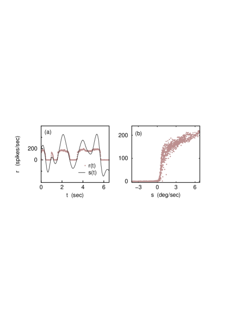
FIG. 1.: Firing rate of H1 as a function of time, averaged over trials: $r(t)=\langle\rho(t)\rangle$ [dots], compared to the input signal $s(t)$ [solid line], for a slow signal (a) and a fast signal (c). We repeat the signal many times to obtain a sampling of the noise ensemble. The units of velocity are spacings of the compound eye’s lattice (ommatidia) per second.

It should be noted that the response function of the neuron $f(\cdot)$ is not a fixed property, but may change with external conditions. The theory presented here is valid within a steady state, in which $f(\cdot)$ takes a particular form and does not change with time. Rather than being a limitation, the context-dependence of $f(\cdot)$ opens the possibility to investigate adaptive changes in the neural response, when adjusting to different steady states [24].

III The universal regime

In this section we present the statistical theory for the case of a constant input signal, $s(t)\!=\!s$, and a random short correlated noise of arbitrary distribution. The result is a renewal process with special symmetry properties, reflecting the underlying neuronal oscillator. We provide explicit formulas for the correlation function and the number variance. As will be shown in later sections, the results obtained here are valid in a limited time range if the stimulus $s(t)$ is time dependent.

A Distribution of Intervals

The distribution of inter–spike intervals is the distribution of times for which $\Phi(t)=1$. Due to the unidirectionality of the phase diffusion, these times are unique, and so the probability density is simply

$$P(t)~{}=~{}\Bigg{\langle}\delta(t-\Phi^{-1}(1))\Bigg{\rangle}~{} = ~{}\Bigg{\langle}\delta(\Phi(t)-1){\dot{\Phi}}(t))\Bigg{\rangle}.$$ (14)

It is more convenient to calculate the cumulative distribution,

$$F(t)~{}=~{}\int_{0}^{t}P(t^{\prime})dt^{\prime}$$ (15)

which can be expressed in terms of the step function, $\Theta$, and its Fourier transform:

$$F(t)=\langle\Theta(\Phi(t)-1)\rangle~{}=~{}\int_{-\infty}^{\infty}\frac{dp}{2\pi ip}e^{-i2\pi p}\langle e^{i2\pi p\Phi(t)}\rangle.$$ (16)

Using the Gaussian approximation (8) for $\Phi(t)$, we find that

$$F(t)~{} = ~{}\int_{-\infty}^{\infty}\frac{dp}{2\pi ip}e^{i2\pi prt-2\pi^{2}p^{2}Dt}$$ (17)

$$= \frac{1}{2}\left(1+\mbox{erf}\left(\frac{rt-1}{\sqrt{2Dt}}\right)\right)$$ (18)

and the interval density is

$$P(t)=\frac{rt+1}{\sqrt{8\pi Dt^{3}}}~{}e^{-(rt-1)^{2}/2Dt}.$$ (19)

In Appendix 1 this result is derived for a discrete sum of non-negative random variables, directly from the central limit theorem. The density (19) depends on two parameters, the average firing rate $r$ and the diffusion coefficient $D$, both of dimensionality [time]^-1. In the derivation, we used only the non–negativity of the frequency integrator to write down Eq. (14), and the Gaussian approximation (8) for $\Phi(t)$; therefore changes in the model which retain these properties will not affect the interval density. Eq. (19) is similar to the first passage time of the Wiener process [7, 31]: it has the same exponent, but this exponent is multiplied by a different function of $t$. As will be shown below, this results in significantly different symmetry properties of the function.

To understand the qualitative properties of the point process, it is convenient to examine it in dimensionless time units, namely to define the time such that the average rate is 1. We denote this time as $x\!=\!rt$. In this representation, the statistics depend on one dimensionless parameter, $\gamma$,

$$\gamma=\frac{D}{r}=\frac{\tau_{n}\langle\delta f^{2}\rangle}{\langle f\rangle}$$ (20)

and the interval density is

$$P(x)=\frac{x+1}{\sqrt{8\pi\gamma x^{3}}}e^{-(x-1)^{2}/2\gamma x}.$$ (21)

The parameter $\gamma$ governs the decay of the interval density both near the origin and at large $t$. For small $\gamma$ these decays are strong, indicating a narrow density, and for large $\gamma$ they are weaker and the distribution is broader. More formally, the moment generating function, $G(\lambda)=\langle e^{-\lambda x}\rangle$, of (21) can be calculated using the integral representation,

$$P(x)=\int_{-\infty}^{\infty}dp(1+i\pi\gamma p)e^{i2\pi(x-1)p-2\pi^{2}\gamma p^{2}x}.$$ (22)

The result is

$$G(\lambda)=\frac{1}{2}\left(1+\frac{1}{\sqrt{1+2\lambda\gamma}}\right)e^{\frac{1}{\gamma}(1-\sqrt{1+2\lambda\gamma})},$$ (23)

and the first two moments are

$$\langle x\rangle = 1+\gamma/2$$ (24)

$$\langle\delta x^{2}\rangle = \gamma+\frac{5}{4}\gamma^{2}.$$ (25)

Note that the average interval length is not equal to the inverse of the average rate, which is 1 in our units. In general, inversion does not commute with averaging; for small $\gamma$, however, the inverse average and the average of the inverse are similar.

Defining the coefficient of variation by $\sqrt{\langle\delta x^{2}\rangle}/\langle x\rangle$ [34], it is seen that the coefficient of variation is approximately proportional to $\sqrt{\gamma}$ for small $\gamma$, and to $\gamma$ for large $\gamma$. It can take on arbitrarily small and large values dependent upon $\gamma$. This is a more quantitative way of seeing that our family of distributions interpolates between low–variability (or regular) and high–variability (or irregular) limits. It should be noted that this distribution arises from a simple integration model of many independent inputs [35]. As noted already by several authors [12, 8], it is not only the properties of the inputs but also of the internal neural response that determine the degree of irregularity of a spike train. In our model, the parameter controlling this irregularity (20), accounts for both these effects.

The fact that $\gamma$ controls the behavior of the density (21) at both tails, takes the quantitative form of an invariance under the transformation $x\to 1/x$, with the Jacobian properly accounted for. This implies that the cumulative distribution of the intervals between successive spikes is identical to the distribution of inverse intervals, when both are measured in dimensionless units. Since our spike train is a renewal process, this invariance of the interval distribution implies an invariance of the process as a whole. In general, for a point process with time intervals $\{x_{i}\}$, one may construct the dual process with intervals $\{1/x_{i}\}$; this has the natural interpretation of local frequencies. The process defined by (21) is self-dual: all statistical properties of the dual process are identical to the original one. For the process defined by (19), this invariance holds up to a global rescaling of the axis. Fig. 2 shows that this is indeed a property of the measured data: the cumulative distributions of intervals and inverse intervals overlap when plotted in dimensionless units.

FIG. 2.: A symmetry of the spike train point process: the distribution of intervals between neighboring spikes is the same as the distribution of the inverse intervals (local frequencies), up to a constant scaling factor. Data are shown from two experiments with constant velocity stimuli, of magnitude 10.5 (a) and 0.16 (b) deg/s.

A generalization of the interval distribution is the scaled interval distribution of order $k$, defined as the distribution of intervals between pairs of spikes that have exactly $k-1$ other spikes in between them. In their landmark paper, Gerstein and Mandelbrot (1964) observed that the scaled interval distributions of low orders in spike trains from the cat cochlear nucleus, have a similar shape. This observation motivated them to suggest the random walk model for the membrane voltage. In our model, we can calculate the scaled interval distribution directly: it is the distribution of times for which $\Phi(t)=k$,

$$F_{k}(t)~{}=~{}\frac{1}{2}\left(1+\mbox{erf}\left(\frac{rt-k}{\sqrt{2Dt}}\right)\right).$$ (26)

In this notation, the interval distribution of Eq. (19) is the scaled distribution of order $1$. Figure 3a shows the first three scaled interval distributions, as measured experimentally, together with Eq. (26). The two fitting parameters of the theory, the average rate $r$ and the diffusion constant $D$, are fitted once for all three graphs. According to the observation of Gerstein and Mandelbrot, these curves should have the same shape after rescaling the time axis to dimensionless units $rt/k$. Figure 3b shows the scaled interval distributions in dimensionless time units. These curves have a similar shape, but do not quite overlap. As is easily seen from Eq. (26), the transformation $t\to t/k$ gives a function of the same general form, but with a different value of $D$. Thus the family of curves $F_{k}(t)$ with parameters $r,D$ obey the following equation:

$$F_{k}^{(r,D)}(t/k)~{}=~{}F_{1}^{(r,\frac{D}{k})}(t),$$ (27)

where the superscripts denote the dependence on the parameters. In Figure 3b, it is clearly seen that the steepness of the curve increases with increasing $k$, consistent with a decrease in the diffusion constant $D$. The point $rt/k=1$ is where the distributions cross, in agreement with the theoretical equation (27).

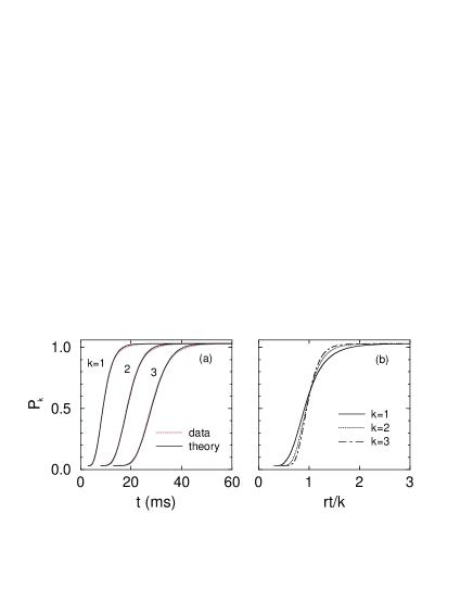
FIG. 3.: (a) Scaled interval distributions of orders $k=1,2,3$, representing the probability of finding a pair of spikes at a given time interval, with exactly $k-1$ spikes in between. Data are shown in grey dotted lines, while theory (Eq. 26) is shown in a solid black line. Fitting parameters of the theory, $r$ and $D$, are fitted once for all three curves. (b) Scaled interval distributions in dimensionless time units. In agreement with Eq. (27), these curves are similar but have slightly different slopes, corresponding to an effective value of $D$ which depends on $k$. The curves cross at $rt/k=1$, as predicted by Eq. (27).

The derivation of the interval density is independent of many microscopic details of the neuron and of the noise, and it is therefore expected to describe correctly the behavior of many different systems. Figure 4 shows a comparison of the interval distribution (19) with experimental data from different parts of the visual system in several animals. Figure 4a shows data measured in our experiment on the motion sensitive neuron H1 in the visual system of the blowfly. In this experiment, the fly watched a random pattern of dark and light bars moving at a constant velocity of $\sim 0.16$ deg/sec. The best fit to the data was found with an irregularity parameter of $\gamma=0.1$. Figure 4b is adapted from data published by Robson and Troy (1987). In this experiment, a stationary sinusoidal grating was presented to an anesthetized cat, and spikes were recorded from neurons in the retina. The particular neuron these data were recorded from was identified as a “Q-type” neuron, characterized by regular spiking. The best fit of Eq. (19) was obtained with $\gamma=0.015$. Figure 4c shows data measured from isolated goldfish retina by Levine and Shefner (1977) in darkness. These data are well described by Eq. (19) with $\gamma=0.1$. Figure 4d contains data measured by Cattaneo et al. (1981) from visual cortex of anesthetized cat, in response to a drifting sinusoidal grating. This interval density is best fit with $\gamma=0.3$.

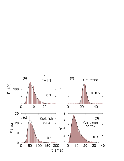
FIG. 4.: Distribution of intervals between neighboring spikes, experiments and theory. The data are from different sensory systems in different animals: (a) fly visual system (lobula plate motion detector), (b) Cat retina, (c) goldfish retina (d) cat visual cortex. For more details about these published data see text. The y-axis is the probability of seeing an interval, in units of 1/s (a-c), and the relative probability in percent (d). The solid black lines are a fit of Eq. (19), and number in each panel indicates the value of the irregularity parameter $\gamma$ in the fit.

These data indicate that the classification of spike trains to universality classes according to the irregularity parameter $\gamma$ is a useful one, and can be applied to many systems. Systems with very different microscopic properties can belong to the same universality class, and their interval density is well described by a theory with one dimensionless parameter. It will be shown in section 4, that this classification can be applied also under conditions of rich dynamic stimuli; in this case, the internal irregularity parameter $\gamma$ describes the statistical properties on short time scales.

B Correlation function

An important statistical property of the spike train is its (auto)-correlation function, $\langle\rho(t)\rho(0)\rangle$. Whereas many models have been used to calculate the interval density, less attention has been paid to the correlation function [16]. In Appendix B we derive the correlation function under the assumption that the noise correlation time $\tau_{n}$ is much shorter than the typical interval between spikes $1/r$. The result is:

$$\langle\rho(t)\rho(0)\rangle = r\delta(t)~{}+~{}r\sum_{k\neq 0}P_{k}^{(r,D)}(|t|)$$ (28)

where $P_{k}^{(r,D)}(t)$ are the densities derived from the scaled interval distributions of Eq. (26),

$$P_{k}^{(r,D)}(t)~{}=~{}\frac{d}{dt}F_{k}^{(r,D)}(t)~{}=~{}\frac{rt+k}{\sqrt{8\pi Dt^{3}}}~{}e^{(rt-k)^{2}/2Dt}.$$ (29)

It is convenient to think about the probability per unit time of finding a spike at time $t\neq 0$, conditional on the event that a spike is found at time $t=0$. This quantity $R(t)$ is proportional to the correlation function in the region $t\neq 0$, and is called the conditional rate:

$$R(t)~{} = ~{}\sum_{k\neq 0}P_{k}^{(r,D)}(|t|)~{}\equiv~{}R_{U}^{(r,D)}(t).$$ (30)

The density labeled $k$ is the probability per unit time for finding a pair of spikes separated by a time $t$ with exactly $(k-1)$ spikes in between. These independent events, when added together, give the total probability per unit time to find a pair of spikes separated by a time $t$, which is just the conditional rate. For small $k$ these individual densities $P_{k}^{(r,D)}$ are narrow and their peaks can be resolved, and as $k\to\infty$ they smear and overlap to give asymptotically $R(t)\sim r$. The degree of regularity, $1/\gamma$, is associated with the number of densities which can be resolved. The notation $R_{U}^{(r,D)}(t)$ is introduced to emphasize that this is a universal function, independent of the detailed neuronal response $f(s)$, and of the detailed properties of the noise. Figure 5 shows the conditional rates for experiments with constant velocity, together with the best fit to Eq. (28). The constant value of the velocity stimulus $s$ increased among parts (a-d) of the figure; the average firing rate $r$ increases and the irregularity $\gamma$ decreases. This is clearly due to refractory effects: as the firing rate increases, the repulsive interaction among the spikes becomes more important, and the spike train becomes more stiff, causing a more regular behavior. The form of the repulsive interaction and the function describing the correlation function, however, remain the same.

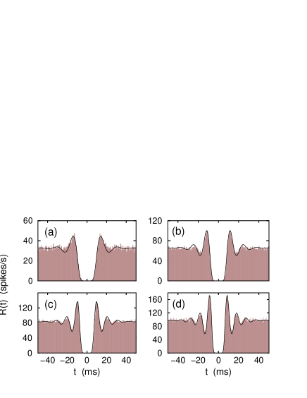
FIG. 5.: Conditional rate for the spike train in experiments with a constant velocity stimulus. Data are shown by a gray histogram, calculated directly from the spike times by binning them into 4 ms bins. Theoretical expression (Eq. 28) is shown by a solid black line. The four parts of the figure correspond to different values of the constant velocity stimulus: 0.7 (a), 2.6 (b), 10.5 (c) and 42.2 (d) deg/sec. As the motion signal becomes stronger, the average firing rate increases and the irregularity parameter decreases (see also Fig. 6).

C Number variance

The number variable $N(t)$ is a random function which counts the number of spikes in the time window $[0:t]$. Defined by

$$N(t)~{}=~{}\int_{0}^{t}\rho(t^{\prime})dt^{\prime},$$ (31)

it provides a useful, less detailed, characterization of the spike train point process. To study the statistics of this variable, we write it as:

$$N(t)=\sum_{k=1}^{\infty}\Theta(\Phi(t)-k)=\mbox{Int}(\Phi(t))$$ (32)

where Int$(y)$ is the integer part of $y$. Its Fourier representation is

$$N(t)=\Phi(t)+\frac{1}{2}-\varphi+\sum_{m\neq 0}\frac{1}{2\pi im}~{}e^{i2\pi m(\Phi(t)+1-\varphi)}$$ (33)

where $\varphi$ is uniformly distributed on $[0,1]$, accounting for a random position of the first spike in a window (see App. C). The number mean is $\langle N(t)\rangle=rt$, and around this mean $N(t)$ fluctuates. Since the correlation function of spikes is of finite range, the long time asymptotic behavior of the number variance is diffusive: $\sigma^{2}_{N}=\langle\delta N^{2}(t)\rangle\sim Dt$ [1]. It is of interest, however, to derive a complete expression for this quantity also for short times, where correlations between spikes are important. Using (33), it is shown in Appendix C that

$$\sigma^{2}_{N} = Dt+\sum_{m=1}^{\infty}\frac{1}{(\pi m)^{2}}\left[1-\cos(2\pi mrt)~{}e^{-2\pi^{2}m^{2}Dt}\right].$$ (34)

Written as function of the number mean, i.e. as a function of the dimensionless time variable $x\!=\!rt$, the number variance is:

$$\sigma^{2}_{N}~{}=~{}\gamma x+\sum_{m=1}^{\infty}\frac{1}{(\pi m)^{2}}\left[1-\cos(2\pi mx)e^{-2\pi^{2}m^{2}\gamma x}\right].$$ (35)

Figure 6 shows the number variance as a function of the number mean, as calculated from an experiments with constant velocity stimuli. Part (a) shows a scatter-plot of the values obtained in various windows in the experiments, with a line showing the average. Part (b) of the figure shows a detailed view of one such average plot, with the theoretical prediction Eq. (35) in solid black line. The number variance of a Poisson process is shown for comparison. The “diffusion constant” in the number variable is $\gamma$, implying again its role as an irregularity parameter: the more stochastic the point process, the faster is the diffusion in the number variance. Similar to Figure 4, a higher constant signal induces a higher firing rate and a lower irregularity of the spike train. Although the data presented here have $\gamma<1$, this is not a fundamental property of the theory, and in general, $\gamma$ can take on also values larger than 1, resulting in a “super-Poisson” behavior.

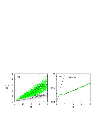
FIG. 6.: Number variance as a function of number mean. (a) Scatter plots of variances, as calculated in different time windows in the experiment. Data are shown from two experiments, with constant velocities of 0.054 and 0.162 deg/s. Solid lines indicate the average value of the variance for a given mean. (b) Comparison to theory: the average value at each number mean, is compared to the theoretic formula (Eq. 35), which is shown by a solid black line. In this experiment, the velocity was 0.162 deg/s.

D Irregularity and stiffness of spike trains

We have presented a statistical theory for a frequency integrator model under constant stimulation and short-range correlated noise. This results in a renewal point process, with the density of intervals given by Eq. (19). This process is characterized by an irregularity parameter $\gamma$, which depends both on the variance of the noise and on the sensitivity of the frequency response to noise; it is the depth of frequency modulation, resulting from these two effects, that determines the irregularity of the process. This one-parameter family of processes can describe many different spike trains, ranging from almost periodic to almost Poisson.

In the data presented above, a correlation was found between the global average firing rate and the irregularity $\gamma$. Figure 7 shows a plot of the different values of $\gamma$ obtained by fitting to the equations in this section, for two sets of experiments. The irregularity decreases roughly linearly with the firing rate, with a saturation at very high firing rate. This is the limit where the absolute refractory period is approached. The simple relation between $\gamma$ and $r$ holds only for the case of constant stimuli, where frequency modulations are essentially induced by noise. When these modulations are affected also by a time varying sensory stimulus, very different behaviors is found (see next section).

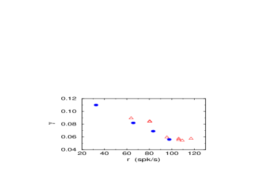
FIG. 7.: Dimensionless irregularity parameter, $\gamma$, as a function of the average firing rate $r$. The different symbols correspond to two different experiments, performed each with a different set of constant velocity signals.

IV Time dependent stimulus

In the previous section, we considered the case of a constant input signal, $s(t)\!=\!s$. More generally signals coming into the system have a temporal structure, and additional time scales enter the problem. If $s(t)$ is slowly varying relative to $1/r$, universal behavior is expected on short times, and slower modulations will appear on longer times. In this section we consider the statistical properties in the case of a slowly varying input signal. We show that the conditional rate can be approximated by a product of the universal function Eq. (30), and a slowly varying envelope reflecting the temporal correlations of the input signal. This envelope is calculated for some simple cases. It is shown that the theory fits the data very well, even when the time scale separation required in theory is only marginally satisfied by the experimental conditions.

A The Telegraph Approximation

Consider a random input signal $s(t)$, that can take on positive as well as negative values. Figure 8 shows a segment of some spike trains recorded from H1 in response to such a stimulus, which was repeated many times. The most striking effect in the figure is the existence of wide regions with spikes, and wide regions which are empty; the typical time for these regions is much larger than the interspike time. This partition into regions is a consequence of the direction selectivity of the H1 neuron: it fires when the effective stimulus is in its preferred direction, and is inhibited by stimulus in the opposite direction. Although the velocity stimulus one the screen varies rapidly in this experiment (every 2ms an independent value is chosen), the spiking and quiet regions in the spike trains have a much slower typical time scale. This results from intermediate processing: the velocity on the screen is not identical to the effective stimulus driving the cell, since it is filtered by the photoreceptors and other elements in the visual pathway.

To describe the phenomenon of spiking regions and quiet regions, we imagine the spike train to be multiplied by a telegraph signal, which keeps track of the algebraic sign of the effective stimulus:

$$\rho(t)\approx\rho^{S}(t)\rho^{E}(t),$$ (36)

where $\rho^{E}(t)=\Theta[s(t)]$ is the telegraphic envelope of the spike train. Figure 8 shows an illustration of the telegraph signal, which demonstrates that the the time scale of the effective stimulus sign change is longer than the typical spike time, $1/r$.

FIG. 8.: Response of the H1 neuron to repeated presentations of a time-dependent stimulus. Each line shows the response to one of the presentations, with the origin $t=0$ corresponding to the onset of the stimulus; each dot represents a spike . The black solid line is an illustration of the telegraphic envelope that multiplies the spike train, due to the strong direction selectivity of the neuron.

Assuming that the telegraph envelope is statistically independent of the short time structure in the spike train, one may write the correlation function as a product,

$$\langle\rho(t)\rho(0)\rangle = \langle\rho^{S}(t)\rho^{S}(0)\rho^{E}(t)\rho^{E}(0)\rangle$$ (37)

$$\approx \langle\rho^{S}(t)\rho^{S}(0)\rangle\langle\rho^{E}(t)\rho^{E}(0)\rangle.$$ (38)

Now brackets $\langle\cdots\rangle$ denote averaging over both the noise and the random stimulus. To perform the averages, we use the separation of time scales: imagine dividing the time axis into blocks of size $\tau_{s}$, the correlation time of the effective stimulus. Performing first the average over the noise in each block separately, the first term in the product gives the correlation function of Eq. (28), with the parameters $r,D$ determined by the local value of $s$:

$$\langle\rho^{S}(t)\rho^{S}(0)\rangle\approx\Bigg{\{}\begin{array}[]{l}r(s)~{}R_{U}^{(r(s),D(s))}(t),~{}~{}~{}~{}~{}~{}~{}~{}~{}~{}\hfill s>0\\ 0,\hfill s\leq 0\end{array}$$ (41)

for $t\neq 0$. If the response is saturated, $r(s)\approx r\Theta(s)$, and the firing rate does not change much inside each spiking region; moreover the diffusion constant $D$ is determined mainly by properties the noise, and is the same in all the spiking regions. Therefore, on averaging the first term over $s$, one has $\alpha R_{U}^{(r,D)}$, where $\alpha$ is the coverage fraction, defined as the fraction of time in which the stimulus is positive ($\langle\rho^{E}(t)\rangle=\alpha$).

The second term in the product (38) is a correlation function of the input signal as seen through the telegraphic envelope:

$$\langle\rho^{E}(t)\rho^{E}(0)\rangle=\langle\Theta[s(t)]\Theta[s(0)]\rangle.$$ (42)

Special care should be taken around the point $t=0$, since it is affected by the delta function singularities. The whole correlation function then takes the form

$$\langle\rho(t)\rho(0)\rangle~{}~{}\approx~{}~{}r\alpha\delta(t)~{}+~{}rR_{U}^{(r,D)}(t)~{}\langle\Theta[s(t)]\Theta[s(0)]\rangle,$$ (43)

and the conditional rate is

$$R(t)~{}~{}=~{}~{}R_{U}^{(r,D)}~{}\langle\Theta[s(t)]\Theta[s(0)]\rangle.$$ (44)

This formula expresses the conditional rate as a product of two terms. The first term reflects internal properties of the noise and of the neuron, similar to the result of the previous section; $R_{U}$ is parameterized by an effective rate $r$ and diffusion constant $D$. This function has an oscillatory structure on a time scale $1/D$, which thus defines the universal regime of the correlation function, in which properties of the inputs do not have an important effect. The second term contains information about statistics of the incoming stimulus, as seen through the nonlinear response of the neuron. It modulates the universal function with a slower structure. Intuitively, the condition of time scale separation can be understood as follows: on short times, $t\leq 1/D$, the envelope is almost constant and the oscillations of the universal part are visible. As these oscillations decay, on times $t>1/D$, the stimulus induced structure sets in. The independence between the two factors affecting the probability of finding a spike at time $t$ given a spike at time $0$, results in a product form.

Eq. (42) indicates that in the telegraph approximation, the envelope of the correlation function depends on the statistics of the zero-crossings of the stimulus. These statistics for a random continuous function are in general very difficult to calculate [17]. Here we need only the correlation function of the algebraic sign of a random signal, and we can proceed in two ways. In the next sub-section we consider the case in which zero crossings are independent, and the resulting correlation function is a simple exponential. Another simplification occurs if the incoming stimulus has Gaussian statistics, and in this case one may derive an exact formula for the correlation function of the nonlinear rate.

B Random independent spiking regions

Let us first assume that the spiking regions occupy random independent positions along the time axis, with lengths $\Delta$ drawn independently from some distribution. This is a crude approximation that may not be justified for many experimental conditions. However, it is the simplest type of telegraphic signal, and is characterized by a small number of parameters; therefore we use this approximation as a starting point. The correlation function of such a telegraph signal is derived in Appendix D, and the result is,

$$\langle\rho^{E}(t)\rho^{E}(t^{\prime})\rangle = \alpha^{2}\frac{\alpha}{\mu}\int_{|t\!-\!t^{\prime}|}^{\infty}p(\Delta)(\Delta-|t\!-\!t^{\prime}|)d\Delta$$ (45)

where $p(\Delta)$ is the distribution of lengths of positive regions in the telegraph signal, and $\mu$ is the average length of such a positive region. The second term clearly decays for $(t\!-\!t^{\prime})\!\to\!\infty$ for a well behaved $p(\Delta)$, and asymptotically there remains only the square of the average signal, $\langle\rho^{E}\rangle^{2}\!=\!\alpha^{2}$. For the case of an exponential distribution of positive regions,

$$p(\Delta)=\frac{1}{\mu}e^{-\Delta/\mu},$$ (46)

the correlation function is also exponential,

$$\langle\rho^{E}(t)\rho^{E}(t^{\prime})\rangle=\alpha^{2}+\alpha\mu e^{-(t\!-\!t^{\prime})/\mu}.$$ (47)

The exponential decay of the envelope, Eq. (47), gives a good fit to many of the measured data sets. It has additional fitting parameters, $\alpha$ and $\mu$, which are the coverage fraction and average length of the positive regions in the telegraph envelope of the spike train. It uses no prior knowledge of the input stimulus, and relies primarily on the direction selectivity of the response. Figure 9 shows the correlation function calculated from spike trains, in two experiments with random signals, of 20Hz (a,b) and 500Hz (c,d) bandwidth. Although in these experiment we know the properties of the visual stimulus presented to the fly, this stimulus is rapid, and pre-processing takes place in earlier stages of the visual pathway; the effective signal entering the H1 neuron is therefore a filtered and probably distorted version of the motion on the screen. Therefore, we try the simple picture of the telegraph approximation, rather than rely on the detailed properties of the visual stimulus. The black solid line in Figure 9 is a fit to a product of the universal function and the envelope correlation in the telegraph approximation, (47). The time scale of the exponential decay is $\mu\approx 50$ms for the slower varying stimulus, and $\mu\approx 20$ms for the faster varying one. In the case of the fast stimulus, the correlation is probably limited by the filtering processes in the visual system, thus indicating that the time scale for these processes is $\approx 20$ms. This is on the order of the behavioral time scale for changes in flight course in these flies, found by Land and Collett (1974) to be $\approx 30$ms.

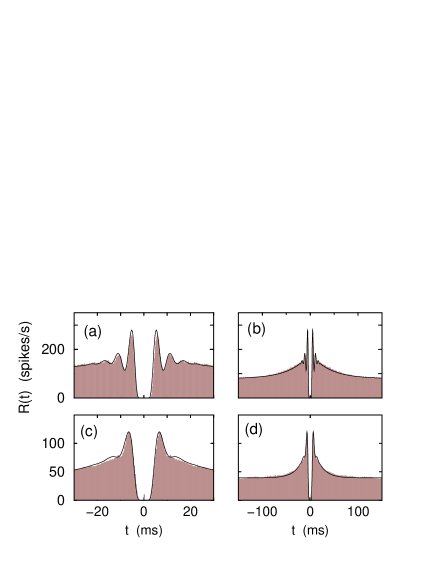
FIG. 9.: Conditional rates for spike trains, in the short time and long time regimes. Data (gray histogram) are measured in experiments where the visual stimulus was a pattern of light and dark bars moving with a random time-dependent velocity. The velocity signal has different bandwidths, of 20 Hz (a,b) and 500 Hz (c,d). The theoretic formula of Eq. (47) is presented as a solid black line.

C A Gaussian input signal

If the incoming random signal is drawn from a Gaussian distribution, one may calculate exactly the correlation function of a nonlinear response $r(s)$. We focus on the simple case where the response is a step function at zero, and the stimulus has zero mean, corresponding to a coverage fraction of $\alpha=1/2$. In this case,

$$\langle\Theta[s(t)]\Theta[s(0)]\rangle=\frac{1}{4}+\frac{1}{2\pi}{\rm arcsin}(|c(t)|),$$ (48)

where $c(t)=\langle s(t)s(0)\rangle$ is the correlation function of the Gaussian signal. In principle, one may calculate the correlation function of a general nonlinear response $r(s)$ in the Gaussian case, but for our purposes it is sufficient to consider the step response. We expect that in an experiment where the driving stimulus varies slowly, the effect of intermediate filters will be negligible and one can take the motion on the screen to be essentially equivalent to the stimulus $s(t)$ driving the neuron. Figure 10 shows the correlation function measured from an experiment where the input signal was a slowly varying random function of time, with a Gaussian distribution. The correlation function as calculated from the data is shown as a gray histogram, whereas the solid black line is given by

$$R(r)=rR_{U}^{(r,D)}\left[\frac{1}{4}+\frac{1}{2\pi}{\rm arcsin}(|c(t)|)\right],$$ (49)

where $c(t)$ was taken from the known distribution of the input signal. The two fitting parameters are $r$, related to the global firing rate, and $D$, the diffusion constant in the universal regime.

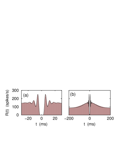
FIG. 10.: Conditional rate for spike trains, in the short time and long time regimes. Data (gray histogram) are measured in experiments where the visual stimulus was a pattern of light and dark bars moving with a random time-dependent velocity, which is very slow and has a Gaussian distribution. The theoretic formula of Eq. (49) is presented as a solid black line.

D Linear rectifier approximation

In analogy to Eq. (43), one expects that if the nonlinear response of the neuron is $f(\cdot)$, the conditional rate will take the form

$$R(t)~{}~{}\approx~{}~{}R_{U}^{(r,D)}~{}\langle r[s(t)]r[s(0)]\rangle$$ (50)

where $r(s)$ is the firing rate as a function of stimulus, obtained by averaging over noise only, and $r,D$ are some effective global parameters representing an average over different regimes where $s$ is almost constant. In this section we show results from experiments where the response $r(s)$ cannot be approximated by a step function, and apart from the direction selectivity the firing seems to follow the input stimulus linearly. A better approximation for the response would therefore be a linear rectifier. We used sine wave stimuli of different amplitudes and periods. Figure 11 shows the firing rate averaged over noise, together with the stimulus, for one such experiment.

FIG. 11.: Stimulus and average response for a sine wave experiment. A random pattern of dark and light horizontal lines was moved by a sine wave velocity (solid black line), and this stimulus was repeatedly presented to the fly. The average firing rate was calculated over the repeated presentations as a function of time (circles). The response of the neuron is not saturated, and it follows closely the positive part of th sine wave stimulus. (Compare the saturated response in Fig. 1a).

We used the approximation

$$r(s)\approx s\Theta(s)$$ (51)

to evaluate the envelope of the conditional rate $\langle r[s(t)]r[s(0)]\rangle$. For a sine wave stimulus of frequency $\Omega$, a straightforward calculation yields

$$\langle r[s(t)]r[s(0)]\rangle=\frac{1}{2}\cos(\Omega|t|)\Bigg{[}\frac{\pi}{\Omega}-|t|\Bigg{]}+\frac{1}{2\Omega}\sin(\Omega|t|).$$ (52)

The conditional rate is, then, given by Eq. (50), with Eq. (52) as the envelope. If we use our knowledge about the frequency of the input signal, we expect to get a description of the conditional rate with only the universal fitting parameters $r$ and $D$, and no additional parameters for the envelope. Figure 12 shows two correlation functions for the sine wave experiments, in the universal (a,c) and the stimulus-dependent (b,d) regimes. No additional parameters of the stimulus other than its frequency were used; the solid black curve was obtained from Eq. (50) with the envelope given by (52). The periodic nature of the envelope is evident in the data, and the theoretic prediction describes both the short range and the long range features well.

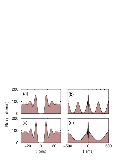
FIG. 12.: Conditional rates for spike trains in the short time and long time regimes. Data (gray histograms) are measured in an experiment where a pattern of dark and light bars were moved horizontally with a sine wave velocity, with periods of 0.25 sec (a,b) and 0.5 sec (c,d). Theory (black solid lines) is obtained from Eq. (50), with the fitting parameters $r$ and $D$, and using the known frequency of the stimulus.

E Irregularity and stimulus properties

In this section, we showed that the conditional rate of the spike trains has approximately a product form. One term in the product is very similar to the conditional rate for a constant stimulus, and describes the behavior on short times. This term is universal in the sense that it depends on only two simple parameters, the global average rate and the internal irregularity of firing. The other term carries information about temporal correlations in the stimulus, and is a long-time envelope over the universal term. We have shown how this envelope can be calculated in several cases, giving a very good fit of the data.

A naive quasi static application of the universal theory would tell us that the short-time behavior is characterized by local values of the parameters $r,D$, and that these change slowly as the external stimulus varies slowly. This seems inconsistent with the short time behavior exhibited by the data (Figures 8a, 10a, 10c). If the parameters would change with the local changes of the external stimulus, the oscillatory structure defined by a period of $r$ would be considerably washed out when averaged over the different values of $s$. The data, however, show pronounced oscillations with a well defined period. This is consistent with the notion that in a changing environment, the system achieves a steady state with the distribution as a whole, thus obtaining global values for the statistical parameters of its firing.

Further evidence for this picture is given by Figure 13, where the correlation function is plotted in normalized time units, and is normalized by the height of the first peak. After rescaling of the two axes, there is only one dimensional parameter describing the short time behavior: the irregularity $\gamma$. Although the correlation functions were measured under different experimental conditions of time varying stimuli, the curves are approximately overlapping in the short time regime $(x<2)$. Thus, under high signal-to-noise ratio, where the frequency modulations are mainly induced by the stimulus and not by the noise, the system tends to fix the internal irregularity parameter $\gamma$ at some preferred value. This cannot be explained by a simple quasi static behavior; it probably involves subtle adaptive mechanisms of the neuron which try to maximize the dynamic range in each stimulus ensemble. This subject is currently under further investigation [24].

FIG. 13.: correlation functions from different experiments with different time-varying stimuli, in dimensionless units. The overlap at short times indicates that the parameter left after rescaling, the internal irregularity, is similar in all these cases.

V Discussion

The statistical properties of spike trains generated by a sensory neuron under various stimulation conditions were considered. Experiments were performed in vivo on a blowfly, where the visual stimulus was well controlled, and spike trains were measured extracellularly from an identified motion sensor. This neuron is known to respond to wide field horizontal motion.

The main theoretical questions addressed were: (i) how does the statistical behavior of spike trains in vivo relate to the biophysics of the spike generation mechanism in the cell, and (ii) how can the effects of internal properties be separated from those induced by the external sensory stimulus (or the input to the neuron). These questions were addressed within the framework of a model, which describes the neuron as a nonlinear oscillator driven both by noise and by an external stimulus. In general the effect of these two is the same: to cause frequency modulations in the oscillator. We considered here the case where the noise and the stimulus are very different in their temporal characteristics, namely the noise is rapid and the stimulus is slow, compared to the time scales typical of the spiking. This separation of time scales enables the theoretic analysis of the model, which in turn provides an understanding of how the different factors are reflected in the statistical properties of the spike trains.

It was found that on the time scale of a few spikes, statistical behavior is rather universal and can be described by a renewal process. This process is derived from phase diffusion of a nonlinear oscillator, and has special symmetry properties reflecting the underlying oscillator. It is characterized by one dimensionless parameter which represents the internal degree of irregularity of the process. This parameter interpolates between highly regular and highly stochastic limits. The parametrizaion allows spike trains from different parts of the visual system, and even from different organisms, to be classified in a simple way.

On the time scale of many spikes, effects of the sensory stimulus become important and are reflected in the form of a slowly varying envelope which modulates the universal functions. Using only simple features of the nonlinear neuronal response, the theory provides quantitative predictions for the statistical properties, which are found to be in very good agreement with our measured data in both the short time and the long time regimes.

Justification for assuming a separation of time scales between noise and stimulus comes from the fact that signals in the visual system are filtered, and therefore the effective signals reaching an interneuron are relatively slow. As often is the case in comparing theory and experiment, we found that the agreement of the theoretical predictions with the data extend to a regime where the required separation of time scales is only marginally satisfied by the experimental conditions.

The understanding of how the stimulus is reflected in the statistical properties of the spike train could be used “backwards”: in cases where little is known about the stimulus, analysis of the long time behavior of the correlation function can give us information about the time scales involved in this stimulus, with only a gross description of the neural response (direction selectivity, degree of saturation). Possibly this understanding can be extended to cross-correlation between several neurons; in that case the separation between stimulus-induced and internal properties will be important in assessing the connections between the neurons. This is subject for future research.


Appendix A

In this Appendix we show that for a unidirectional random walk, (a “thermal ratchet” walk), the density of times between barrier crossing is given by Eq. (21), in the limit where many steps are needed to cross the barrier.

We consider the discrete case. Let $x_{i}$ be non–negative random variables ($x_{i}\geq 0$), identically distributed and independent, with $\langle x\rangle=\mu$ and $\langle\delta x^{2}\rangle=\sigma^{2}$. Define the random variable of their sum as

$$X_{N}=\sum_{i=1}^{N}x_{i}.$$ (A.1)

Let $C$ be a constant positive number, then for large enough $N$ one has from the central limit theorem,

$${\rm Prob}\{X_{N}\leq C\} = \frac{1}{\sqrt{2\pi N\sigma^{2}}}\int_{-\infty}^{C}\exp\{-\frac{(X_{N}-N\mu)^{2}}{2N\sigma^{2}}\}$$ (A.2)

$$= \frac{1}{2}\left[1+{\rm erf}\left(\frac{C-N\mu}{\sqrt{2N\sigma^{2}}}\right)\right]$$ (A.3)

where ${\rm erf}(x)=\frac{2}{\pi}\int_{0}^{x}e^{-t^{2}}dt$. Now define $N_{1}$ to be the number of steps required to first reach the barrier. Then from the non–negativity it follows that

$${\rm Prob}\{X_{N}\leq C\}={\rm Prob}\{N_{1}\geq N\}=1-{\rm Prob}\{N_{1}\leq N\}.$$ (A.4)

There are some normalization subtleties here, but let us imagine that the sample space is composed of trajectories with a finite number of steps $M$ which is much larger than the typical number needed to cross threshold. Then,

$${\rm Prob}\{N_{1}\leq N\}~{}=~{}\frac{1}{2}\left[1+{\rm erf}\left(\frac{N\mu-C}{\sqrt{2N\sigma^{2}}}\right)\right].$$ (A.5)

Appendix B

In this Appendix, we derive Eq. 28. Starting from the definition,

$$\langle\rho(t)\rho(0)\rangle~{}~{}=~{}~{}\Bigg{\langle}\sum_{k,l}\delta(\Phi(t)-k)\delta(\Phi(0)-l)\dot{\Phi}(t)\dot{\Phi}(0)\Bigg{\rangle}.$$ (B.1)

The term at $t=0$ must be taken care of separately: it corresponds to $k=k^{\prime}$,

$$\sum_{k}\Bigg{\langle}\delta\Bigg{(}\Phi(t)-k\Bigg{)}\delta\Bigg{(}\Phi(t)-\Phi(0)\Bigg{)}\Bigg{\rangle}\dot{\Phi}(t)\dot{\Phi}(0)$$ (B.2)

$$= \sum_{k}\Bigg{\langle}\delta\Bigg{(}\Phi(t)-k\Bigg{)}\frac{\delta(t)}{\dot{\Phi}(t)}\dot{\Phi}(t)\dot{\Phi}(0)\Bigg{\rangle}$$ (B.3)

$$= \delta(t^{\prime})\sum_{k}\Bigg{\langle}\delta\Bigg{(}\Phi(t)-k\Bigg{)}{\dot{\Phi}(t)}\Bigg{\rangle}$$ (B.4)

$$= r~{}\delta(t),$$ (B.5)

As expected for a point process of average rate $r$. For times $t\neq 0$, we calculate the conditional rate $R(t)$, the probability of firing at some time $t$ given a spike at time $0$:

$$R(t) = \sum_{k\neq 0}\langle\delta(\Phi(t)-k){\dot{\Phi}(t)}\rangle$$ (B.6)

$$= \sum_{k\neq 0}\frac{d}{dt}\langle\Theta(\Phi(t)-k)\rangle.$$ (B.7)

Using the integral representation of the Theta function, we write

$$R(t)=\sum_{k\neq 0}\frac{d}{dt}\int_{-\infty}^{\infty}\frac{dp}{2\pi ip}e^{-i2\pi k}\langle e^{i2\pi\Phi(t)}\rangle.$$ (B.8)

As before, we use the Gaussian approximation for $\Phi(t)$, Eq. (8), which is justified for times $t$ satisfying $\tau_{n}\ll t$:

$$R(t) = \sum_{k\neq 0}\frac{d}{dt}\int_{-\infty}^{\infty}\frac{dp}{2\pi ip}e^{i2\pi p(rt-k)-2\pi^{2}p^{2}Dt}$$ (B.10)

$$= \sum_{k\neq 0}\frac{d}{dt}\int_{-\infty}^{\infty}dp\int^{\nu}dye^{i2\pi y-2pi^{2}p^{2}Dt}$$ (B.11)

where $\nu=rt-k$. Doing first the integral $dp$, we find

$$R(t) = \sum_{k\neq 0}\frac{d}{dt}\int^{\nu}\frac{dy}{\sqrt{2\pi Dt}}~{}e^{y^{2}/2Dt}$$ (B.12)

$$= \sum_{k\neq 0}\frac{d}{dt}\left[\frac{1}{2}\mbox{erf}\left(\frac{\nu}{\sqrt{2Dt}}\right)+\mbox{const}\right]$$ (B.13)

$$= r\sum_{k\neq 0}\frac{t+k/r}{\sqrt{8\pi Dt^{3}}}e^{(rt-k)^{2}/2Dt}.$$ (B.14)

Appendix C

Here we discuss the properties of the number variable, which counts the number of spikes in the window $[0:t]$. One must specify how the point $t=0$ is chosen, and there are two natural choices: (i) start counting at a spike, and (ii) start counting at a random point in the spike train. The second choice of a random origin is the more commonly used. In this case, it is convenient to define an auxiliary variable $\varphi=\Phi(t_{1})$, the phase of the integrator $\Phi(t)$ at the time of the first spike in the window. This variable is uniformly distributed in $[0:1]$, and with this we have

$$N(t) = \mbox{Int}[\Phi\!(t)\!+\!1\!-\!\varphi]$$ (C.1)

$$=\Phi\!(t)\! + \!1\!-\!\varphi+\sum_{m=1}^{\infty}\frac{1}{\pi m}\sin[2\pi m(\Phi\!(t)\!+\!1\!-\!\varphi]-\frac{1}{2}.$$ (C.2)

Note that the constant $-\frac{1}{2}$ ensures that $N(0)=0$. Since $\varphi$ only depends on the choice of origin, it is independent of $\Phi(t)$, and therefore

$$\langle N(t)\rangle = \langle\Phi(t)\rangle+\frac{1}{2}-\langle\varphi\rangle+\sum_{m\neq 0}\frac{1}{2\pi im}\langle e^{i2\pi m[\Phi(t)\!+\!1\!-\!\varphi]}\rangle$$ (C.3)

$$= rt+\sum_{m\neq 0}\frac{1}{2\pi im}\langle e^{[i2\pi m[\Phi(t)\!+\!1]}\rangle\langle e^{-i2\pi m\varphi}\rangle$$ (C.4)

$$= rt.$$ (C.5)

Now to calculate the number variance we define the fluctuation

$$\delta N(t)=\delta\Phi(t)+(\varphi-\frac{1}{2})+\sum_{m\neq 0}\frac{1}{2\pi im}e^{i2\pi m[\Phi(t)+1]}$$ (C.6)

and average its square:

$$\sigma^{2}_{N} = \langle\delta N(t)^{2}\rangle=\langle\delta\Phi\!(t)^{2}\rangle+\langle(\frac{1}{2}\!-\!\varphi)^{2}\rangle$$ (C.7)

$$+ 2 \langle\delta\Phi\!(t)(\frac{1}{2}\!-\!\varphi)\rangle+\langle 2(\frac{1}{2}\!-\!\varphi)\sum_{m\neq 0}\frac{1}{2\pi im}e^{[i2\pi m[\Phi\!(t)\!+\!1\!-\!\varphi]}\rangle$$ (C.8)

$$+ \sum_{m,m^{\prime}\neq 0}\frac{1}{(2\pi i)^{2}mm^{\prime}}\langle e^{i2\pi(m+m^{\prime})[\Phi(t)+1-\varphi]}\rangle.$$ (C.9)

By Eq. (9), $\langle\delta\Phi(t)^{2}\rangle\!=\!Dt$; averaging the second term over $\varphi$ gives $\frac{1}{12}$. Due to the independence of $\varphi$ and $\Phi(t)$, the first cross-term vanishes while the second cross-term decouples into

$$-2\sum_{m\neq 0}\frac{1}{2\pi im}\langle e^{[2\pi im[\Phi(t)\!+\!1]}\rangle\langle\varphi e^{-2\pi im\varphi}\rangle.$$ (C.10)

Performing the average over $\varphi$,

$$\langle\varphi e^{-i2\pi m\varphi}\rangle=\frac{d}{d\mu}\frac{1}{2\pi im}\langle e^{-2\pi im\varphi\mu}\rangle\Bigg{|}_{\mu\!=\!1}=\frac{-1}{2\pi im},$$ (C.11)

and we have for the second cross-term

$$\sum_{m\!=\!1}^{\infty}\frac{1}{(\pi m)^{2}}\cos(2\pi mrt)e^{-2\pi^{2}m^{2}Dt},$$ (C.12)

where the Gaussian approximation was used when averaging over $\Phi(t)$. In the last double sum of Eq. (C.9), all terms vanish by averaging over $\varphi$ except for the terms $m+m^{\prime}=0$, which gives

$$\sum_{m\!\neq\!0}\frac{1}{(2\pi m)^{2}}=\frac{1}{12}.$$ (C.13)

Adding the terms together we find

$$\sigma^{2}_{N}=Dt+\frac{1}{6}+\sum_{m\!=\!1}^{\infty}\frac{1}{(\pi m)^{2}}\cos(2\pi mrt)e^{-2\pi^{2}m^{2}Dt}$$ (C.14)

which is the same as Eq. (34).


Appendix D

In this Appendix we derive Eq. (47) for the correlation function of the envelope of the spike train, in the telegraph approximation. The envelope $\rho^{E}(t)$ is composed of a train of characteristic window functions,

$$\langle\rho^{E}(t)\rangle=\sum_{k}\chi\Bigg{(}T_{k}\!-\!\frac{\Delta_{k}}{2},T_{k}\!+\!\frac{\Delta_{k}}{2}\Bigg{)}$$ (D.1)

as illustrated in Fig. 14. This function has a Fourier transform

$$\langle\rho^{E}(\omega)\rangle = \int_{-\infty}^{\infty}\rho^{E}(t)e^{-i\omega t}$$ (D.2)

$$= \sum_{k}e^{-i\omega T_{k}}\frac{\sin(\omega\Delta_{k}/2)}{(\omega/2)}+\alpha\delta(\omega),$$ (D.3)

where $T_{k}$ denote the middle points of the positive signal regions.

FIG. 14.:

These positive regions are assumed to be distributed over the time axis independently with a density $\beta$ per unit time, and with an average length of $\langle\Delta\rangle=\mu$. Averaging in the frequency domain gives

$$\langle|\rho^{E}(\omega)|^{2}\rangle=\beta\frac{\langle\sin^{2}(\omega\Delta/2)\rangle}{(\omega/2)^{2}}+(\beta\mu)^{2}\delta(\omega).$$ (D.4)

In the time domain this expression transform to

$$\langle\rho^{E}(t)\rho^{E}(0)\rangle = (\beta\mu)^{2}$$ (D.5)

$$+ \beta\int_{0}^{\infty}p(\Delta)d\Delta\int_{-\infty}^{\infty}\frac{d\omega}{2\pi}\frac{\sin^{2}(\omega\Delta/2)}{(\omega/2)^{2}}e^{i\omega t}.$$ (D.6)

The last tern in this expression is the Fourier transform of a product of two sinc function, which is the convolution of two square windows. This convolution has the form

$$\chi*\chi=\Bigg{\{}\begin{array}[]{l}0~{}~{}~{}~{}~{},\hfill|t|>\Delta\\ \Delta-|t|,\hfill|t|\leq\Delta\end{array}$$ (D.9)

which is equivalent to Eq. (45).

Acknowledgments
Many thanks to G. Lewen, for preparing the experiments, and to N. Tishby and A. Schweitzer for comments.

REFERENCES

- [1] Spikes: Exploring the Neural Code, F. Rieke, D. Warland, R. de Ruyter van Steveninck and W. Bialek, MIT Press 1997.
- [2] Electric Current Flow in Excitable Cells, J.J.B. Jack, D. Noble and R.W. Tsien, Clarendon Press, Oxford 1975.
- [3] A.L. Hodgkin and A.F. Huxley, J. Physiol. 117, 500 (1952).
- [4] E.D. Adrian, The basis of sensation, Christophers, London (1928).
- [5] Models of the Stochastic Activity of Neurons, A.V. Holden, Lecture Notes in Biomathematics, Springer-Verlag 1976.
- [6] Stochastic Models for Spike Trains of Single Neurons, G. Sampath and S.K. Srinivasan, Lecture Notes in Biomathematics, Springer-Verlag 1997.
- [7] H.C. Tuckwell, Introduction to theoretical neurobiology (Cambridge University Press , 1988).
- [8] A formal reduction of conductance-based models to a phase model is presented in B.S. Gutkin and G.B. Ermentrout, Neur. Comp. 10, 1047 (1998).
- [9] N. Brenner, O. Agam, W. Bialek and R. de Ruyter van Steveninck, Phys. Rev. Lett. 81, 4000 (1998).
- [10] For a review of integrate-to-threshold models, see A.M. Bruckstein and Y.Y. Zeevi, Biol. Cyb. 34, 63 (1979).
- [11] G. Gestri, Biophys. J. 11, 181 (1971).
- [12] T.W. Troyer and K.D. Miller, Neur. Comp. 9, 971 (1997).
- [13] J.G.Robson and J.B.Troy, J. Opt. Soc. America A 4, 2301 (1987).
- [14] A. Cattaneo, L. Maffei and C. Morrone, cells, Proc. R. Soc. Lond. B 212, 279 (1981).
- [15] M.W. Levine and J.M. Shefner, retinal Biophys. J. 19, 241 (1977).
- [16] G. Gestri and P. Piram, Biol. Cybern. 17, 199 (1975).
- [17] S.O. Rice, in Selected papers on noise and stochastic processes, Ed. N. Wax, Dover publications, NY (1954).
- [18] M. F. Land and T. S. Collett, J. Comp. Physiol. 89, 331–357 (1974).
- [19] E. Schneidman, B. Freedman and I. Segev, Neur. Comp. 10, 7, p. 1679 (1998).
- [20] W. Bialek, F. Rieke, R.R de Ruyter van Steveninck, “Reading the Neural Code”, Science 252, 854 (1991).
- [21] N. Franceschini, A. Riehle and A. le Nestour, in Facets of Vision, Edited by D.G. Stavenga and R.C. Hardie (Springer-Verlag, 1989)
- [22] K. Hausen and M. Egelhaaf in Facets of Vision, Edited by D.G. Stavenga and R.C. Hardie (Springer-Verlag, 1989)
- [23] For details see R. de Ruyter van Steveninck and W. Bialek, Phil. Trans. R. Soc. Lond. B (1995) 348, 321.
- [24] N. Brenner, W. Bialek and R. de Ruyter van Steveninck, “Adaptive rescaling of the neural response”, preprint (1999).
- [25] R. de Ruyter van Steveninck and W. Bialek, Proc. R. Soc. Lond. Ser. B 234, 379–414 (1988).
- [26] Z.F. Mainen and T.J. Sejnowski, ”Reliability of Spike Timing in Neocortical Neurons”, Science 268, 1503 (1995).
- [27] W. Bair and C. Koch, ”Temporal Precision of Spike Trains in Extrastriate Cortex of the Behaving Macaque Monkey”, Neur. Comp. 8, 1185 (1996).
- [28] Rob R. de Ruyter van Steveninck, G.D. Lewen, S.P. Strong, R. Koberle and W. Bialek, Science 275, p. 1805 (1997).
- [29] P. Bedenbaugh and G. L. Gerstein, ”Rectification of Correlation by a Sigmoid Nonlinearity”, Biol. Cybern. 70, p. 219 (1994).
- [30] P.I.M. Johannesma, in Neural Networks - Proc. of the School on Neural Networks, Ravello 1967, Ed. E. R. Caianiello, Springer Verlag N.Y. (1968).
- [31] G.L. Gerstein and B. Mandelbrot, Biophys. J. 4, 41 (1964).
- [32] I.F Blake and W.C. Lindsey, Level crossing problems for random processes, IEEE Trans. Info. Th., vol.IT-19, no.3, 295, (1973).
- [33] Statistical Mechanics of Phase Transitions, J. M. Yeomans, Clarendon Press, Oxford 1992. Rev.
- [34] S. Hagiwara, “Analysis of interval fluctuation of the sensory nerve impulse”, Jpn. J. Physiol 4, 234 (1954).
- [35] W.R. Softky and C. Koch, of J. Neurosc. 13, 334 (1993).