A METHOD TO DETERMINE
THE IN-AIR SPATIAL SPREAD OF
CLINICAL ELECTRON BEAMS

Abstract

We propose and analyze in detail a method to measure the in-air spatial spread parameter of clinical electron beams. Measurements are performed at the center of the beam and below the adjustable collimators sited in asymmetrical configuration in order to avoid the distortions due to the presence of the applicator. The main advantage of our procedure lies in the fact that the dose profiles are fitted by means of a function which includes, additionally to the Gaussian step usually considered, a background which takes care of the dose produced by different mechanisms that the Gaussian model does not account for. As a result, the spatial spread is obtained directly from the fitting procedure and the accuracy permits a good determination of the angular spread. The way the analysis is done is alternative to that followed by the usual methods based on the evaluation of the penumbra width. Besides, the spatial spread found shows the quadratic-cubic dependence with the distance to the source predicted by the Fermi-Eyges theory. However, the corresponding values obtained for the scattering power are differing from those quoted by ICRU nr. 35 by a factor $\sim 2$ or larger, what requires of a more detailed investigation.

I INTRODUCTION

Nowadays, electron beams have become a tool widely used in radiation treatment of cancer. However, one of the major difficulties in the daily clinical procedure is the accurate calculation of the electron dose distribution. At present, most of the treatment planning determinations are based on the pencil beam model,[1] which assumes that broad beams are composed by an infinite number of pencil beams, each one spreading as predicted by the Fermi-Eyges multiple scattering theory. In this approach the pencil beams are supposed to present Gaussian distribution profiles in both space and angular coordinates, at any point of their trajectory, and then the corresponding spatial and angular spread parameters are basic ingredients to characterize the beams.

The purpose of this work is to determine the spatial spread parameter in-air, on the beam axis and for various distances to the source.

The usual techniques to obtain the spatial and angular spreads use different relations between the spatial spread and the penumbra width (see e.g. Refs. [1, 2, 3]). However, these procedures present a major problem because of the different definitions of the penumbra width which can be found in the literature. In Refs. [1, 4], it is considered to be the average spatial separation between the 10 and 90% isodose levels. The ICRU [5] recommended the same definition but for the 20 and 80% isodose levels. Finally, in Refs. [2, 3] the penumbra width is obtained as the distance between the intersection of the tangent at the 50% point with the 0%-100% dose levels. In all the cases the measurements refer to a normalized beam profile. The main problem is that the values obtained using the different procedures described above can differ by more than a 30% and therefore the concept of penumbra width is itself misleading.

Besides, the procedure followed in these works presents additional error sources which are neither considered nor discussed. The errors in the measured dose profiles, in the determination of the point of 50% dose and in the calculation of the corresponding tangent are usually forgotten. All these errors sum up increasing the indetermination of the penumbra width, with the consequent ambiguities in the quantities calculated from it [6].

A different approach to the problem is followed by McKenzie [7] and Werner, Khan, and Deibel [8]. In their work these authors measure the electron dose distribution behind the edge of a lead block covering a flat homogeneous phantom in the half plane $x<0$ as in Ref. [3], but they do not determine the penumbra width. Instead, they obtain the spatial spread from Gaussian functions fitted to the corresponding strip beam profiles. These are calculated by deriving the measured dose profiles by means of a two-point difference formula. Unfortunately, each step in this method (the measurement of the dose profiles, the method to obtain the strip profiles and the fit procedure) introduces an error in the results which is not considered at all. All these errors propagate to the final results and it is not possible for the reader to know their accuracy.

In this work we want to address a new procedure to obtain the spatial spread which, as in Refs. [3, 7, 8], is based on measurements performed at the central area of the beam. However, our method uses a simple analytical formalism, is plainly reproducible and shows controlled sources of uncertainty.

The organization of the paper is as follows. In Sect. II we describe the theory underlying the method. Sect. III is devoted to the material and methods used in the experimental side. In Sect. IV we discuss the results. Finally, we give our conclusions in Sect. V.

II THEORY

As mentioned above, our procedure to determine the in-air spatial spread is based on the measurement of the dose profiles generated by an electron beam below a lead block partially collimating it. In this section we justify our methodology.

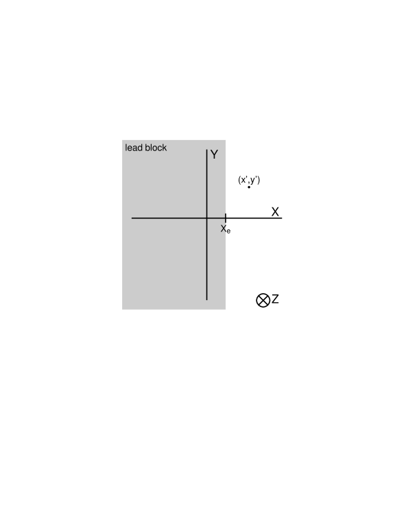
FIG. 1.: Experimental setup considered in our work.

Let us consider the $xyz$-coordinate system depicted in Fig. 1, to which the measurements will be referred. Let us suppose an infinitely broad beam parallel to the $z$-axis and traveling in the direction of increasing $z$. To calculate the dose deposited by the beam at a given point we use the pencil beam model. In this approach, it is assumed that broad beams are formed as the sum of infinite parallel pencil beams, each of them producing dose profiles of Gaussian type at each $z$. Thus, in our case, the ray centered at the point $(x^{\prime},y^{\prime})$ in Fig. 1 gives rise to a profile:

$$D_{(x^{\prime},y^{\prime})}(z,x,y)\,=\,D_{\infty}\,\frac{1}{\sqrt{2\pi}\sigma_{x}(z)}\,\exp\left[-\frac{(x-x^{\prime})^{2}}{2\sigma_{x}^{2}(z)}\right]\,\frac{1}{\sqrt{2\pi}\sigma_{y}(z)}\,\exp\left[-\frac{(y-y^{\prime})^{2}}{2\sigma_{y}^{2}(z)}\right]\,,$$ (1)

where $D_{\infty}$ is a normalization constant which actually gives the broad beam electron dose. The parameters $\sigma_{x}(z)$ and $\sigma_{y}(z)$ label the spatial spreads in the $x$ and $y$ directions, respectively, at a given $z$.

Let us now assume a semi-infinite lead block partially collimating the beam, as shown in Fig. 1. We call $X_{\rm e}$ the $x$-coordinate of the edge of the lead block in our reference system and we fix the $xy$-plane at $z=0$ coinciding with the lower edge of the collimator. We can calculate the total dose distribution in $xy$-plane at a given position $z>0$ as:

$$D(z,x,y) = \int_{X_{\rm e}}^{\infty}{\rm d}x^{\prime}\,\int_{-\infty}^{\infty}{\rm d}y^{\prime}\,D_{(x^{\prime},y^{\prime})}(z,x,y)$$ (2)

$$= D_{\infty}\,\int_{X_{\rm e}}^{\infty}{\rm d}x^{\prime}\,\frac{1}{\sqrt{2\pi}\sigma_{x}(z)}\,\exp\left[-\frac{(x-x^{\prime})^{2}}{2\sigma_{x}^{2}(z)}\right]$$ (3)

$$= D_{\infty}\,\int_{-\infty}^{x}{\rm d}t\,\frac{1}{\sqrt{2\pi}\sigma_{x}(z)}\,\exp\left[-\frac{(t-X_{\rm e})^{2}}{2\sigma_{x}^{2}(z)}\right]$$ (4)

$$= D_{\infty}\,P(x;X_{\rm e},\sigma_{x}(z))\,,$$ (5)

where:

$$P(x;m,\sigma)\,=\,\int_{-\infty}^{x}{\rm d}t\,\frac{1}{\sqrt{2\pi}\sigma}\,\exp\left[-\frac{(t-m)^{2}}{2\sigma^{2}}\right]\,=\,\frac{1}{2}\,{\rm erfc}\left(\frac{m-x}{\sqrt{2}\sigma}\right)$$ (6)

is the cumulative distribution function corresponding to a normal distribution centered at $m$ and with standard deviation $\sigma$ and erfc stands for the complementary error function [9].

It is important to note that, the dose distributions given by Eq. (5) have the same centroid $X_{\rm e}$, independently of the $z$-value at which they are measured. This is so because the beam we have considered up to now is parallel to the $z$-axis of our reference system.

Eq. (5) is valid only when the measurement plane is irradiated by a uniform, semi-infinite broad beam. In actual experiments this is not the case and it is necessary to consider the corresponding corrections.

First of all, it is obvious that the actual beam is finite and, as a consequence, it exhibits a physical end in the open (not collimated) area. This produces a certain distortion in the dose profiles which will differ from the Gaussian shape expected for infinitely broad beams. In order to minimize these differences, we focus our attention on the data acquired below the lead collimator. Therein, we expect to be sufficiently far away from this physical end of the beam and we can assume that the Gaussian approach is enough reasonable to describe the profiles.

On the other hand, the finite dimensions of the source, together with the fact that the distance from the source to the measuring plane is not infinity, make the actual beam to diverge. This gives rise (see e.g. Ref. [2]) to two effects. The first one is that the constant $D_{\infty}$ in Eq. (5) depends on the $z$-value. Then the dose at a given point is:

$$D(z,x,y)\,=\,D_{\infty}(z)\,P(x;X_{\rm e},\sigma_{x}(z))\,.$$ (7)

For electron beams generated in linear accelerators (LINAC), it is possible, in practice, to define a point virtual source. As a consequence, the dependence of $D_{\infty}$ with $z$ must verify the well known inverse squared law. We will check this point a posteriori directly on the measured profiles (see Subsect. IV B).

A second effect of the divergence of the beam in the actual experiment is that, in general, the centroid of the dose distributions will vary with the $z$-coordinate of the measuring plane [2]. Then, the dose profiles will be given by:

$$D(z,x,y)\,=\,D_{\infty}(z)\,P(x;x_{\rm cent}(z),\sigma_{x}(z))\,,$$ (8)

where $x_{\rm cent}(z)$ represents, for each $z$ value, the $x$ position of the centroid of the distribution.

It is worth to point out that only if the $x$-position of the point virtual source of the beam is exactly $X_{\rm e}$, the centroids $x_{\rm cent}(z)$ would be independent of $z$. In such a case these centroids will equal $X_{\rm e}$. It is evident that this situation cannot be ensured in actual experiments; nevertheless, this particular case is included in the general equation (8).

Geometrically, the centroid $x_{\rm cent}(z)$ can be understood as the radiological projection of the edge of the collimator produced by the beam and it is expected to behave linearly with $z$ (see Ref. [2]). An immediate result is that the equation:

$$x_{\rm cent}(z=0)\,=\,X_{\rm e}$$ (9)

must be verified. In our experimental procedure (see Subsect. III A) we measure these positions $x_{\rm cent}(z)$ and we check that they show the required linear behavior and that Eq. (9) is satisfied.

Finally, it is worth to note that, in the actual experiments, measurements are performed by means of an ionization chamber sited in an electro mechanical device which permits the positioning of the chamber. Then, the source-plus-collimator system will not be perfectly aligned, in general, with the coordinate system in which measurements are done. One can expect that this new system is both shifted and rotated with respect to the measurement system and this must be taken into account. However, these effects can be minimized by controlling with the standard procedures (optical, mechanical, etc.) the positioning of the gantry head of the accelerator and we will assume they are incorporated in the values of $x_{\rm cent}(z)$ we determine experimentally.

In view of the previous discussion, the fitting function we adopt to analyze the experimental dose distributions is the following:

$$D_{\rm fit}(z,x)\,=\,D_{\infty}(z)\,P(x;x_{\rm cent}(z),\sigma_{x}(z))\,+\,B(z,x)\,.$$ (10)

We have add the “background” function $B(z,x)$ in order to take care of different contributions to the dose which the Gaussian model does not account for. Thus, part of the dose due to the bremsstrahlung and the dose due to electrons scattered at the gantry head, at the measurement device and its surroundings, as well as those scattered in-air with large angles, are supposed to be described by this function. The particular functional dependence of $B(z,x)$ with $x$ will be considered in Subsect. IV A and its role in the model we propose will be discussed in Subsect. IV C. As we quote below, the contribution of the background is not at all negligible and its consideration in this simple way permits to obtain very good fits of the measured profiles.

III EXPERIMENTAL SETUP

As mentioned above, our interest is to determine the in-air spatial spread of clinical electron beams produced by a linear accelerators. Also, we want to investigate its dependence with the distance to the lower edge of a lead block (actually, the inner jaw) collimating the beam. To do that, we have measured the corresponding relative dose profiles in air by using a Wellhöffer WP-700 system which incorporates an electrometer Wellhöffer WP-5007 and an ionization chamber Wellhöffer IC-10 of 0.12 cm³ sited in an electro mechanical device which permits the tridimensional positioning of the chamber with a theoretical precision of 0.1 mm. The dose profiles have been acquired in continuous mode, by displacing the chamber in the $x$-axis direction (at $y$=0) and for $z$ values ranging between 50 and 80 cm. Beams with nominal energies varying from 6 to 18 MeV generated by a Siemens Mevatron KDS have been considered. This ensures the generality of the results for similar machines. All the profiles obtained have been treated by means of the software package WP-700 Version 3.20.02 accompanying the measurement system.

In our reference system ($z=0$ at the bottom edge of the jaws), the isocenter lies at $z=73$ cm and the scattering foils are sited at $z=-27$ cm.

The reproduction of the conditions established in the theoretical hypothesis was achieved by collimating the beam to the central axis using the adjustable collimators of the LINAC in asymmetric configuration. This point deserves a comment. Electron dose computation programs require as input data the spatial and/or angular spreads of the beam. The usual practice is to determine these parameters below the applicator at treatment distances. In this way, the obtained values are considered to be clinically relevant because the possible modifications in the parameters introduced by the presence of the applicator are taken into account. However, our interest stands for a more basic question. As mentioned in the Introduction, what we want to do is to determine the spatial spread of the beam in order to have more information to characterize it. In this sense we are interested in eliminate all the possibles distortions induced by the use of the different clinical devices. Besides we try in this paper to show the possibilities of the analysis technique we propose and to study its feasibility. We think that the experimental setup we consider provides the cleanest experimental situation to complete our purposes. We leave for a following work the investigation of the behavior of the parameters of interest when applicator and phantom are introduced [6].

A Determination of the position of the centroid, $x_{cent}$

As we have previously discussed, the position of the centroid of the dose distribution shifts in the transverse direction when the beam goes downstream. The procedure we have performed to determined the values $x_{\rm cent}(z)$ at each $z$ is based in a series of measurements done with the following experimental setups:

  

Setup 1. First, we have moved the right collimator to the center (position $X_{\rm e}$) maintaining the left one apart. In this situation we have obtained four dose profiles, without the reference chamber, for each energy and for each of the four values of $z$ selected: 50, 60, 70 and 80 cm. Each profile has been taken crossplane (with $y=0$) and varying $x$ from -2 to 2 cm.

  

Setup 2. Next, we have moved the left collimator to the center. In order to check that beams are completely collimated we have measured four dose profiles for the largest energy (18 MeV) at $z=50$ cm. We have checked that the dose level in this situation is zero. This ensures that the left collimator is at $X_{\rm e}$ also.

  

Setup 3. Finally, we have moved the right collimator apart. With this setup we have got four dose profiles, again without the reference chamber, for each energy and for the same values of $z$ as in Setup 1.

The role of the reference chamber in our procedure deserve some additional explanations. It is obvious that the way we determine the $x_{\rm cent}$ values imposes the necessity of guaranteeing an equal normalization for the profiles obtained in the two asymmetrical configurations corresponding to Setups 1 and 3. However, it has not been possible to situate the reference chamber in a manner that it were irradiated identically in both setups. This is the reason why we switched off it when the profiles used to measure $x_{\rm cent}$ were taken.

The experimental procedure followed (which ensures the absence of radiation when the two collimators are closed in Setup 2) allows us to obtain $x_{\rm cent}$ by finding the cross point between couples of the symmetrical dose profiles measured with Setups 1 and 3. To determine the cross point of a given pair we have, first, calculated the difference between the two profiles of the couple, then found the zero of the resulting function and, finally, checked that the two profiles are symmetric with respect to the cross point. The manipulation of the profiles as described here has been done with the software package WP-700 of the measurement system. The four profiles measured with each one of the Setups 1 and 3, provide us with 16 experimental values of $x_{\rm cent}$ (for each energy and $z$). These values give a sufficient statistics and permit us to calculate the corresponding mean, $\overline{x}_{\rm cent}$, and standard deviation, $\sigma_{{x}_{\rm cent}}$, values. The results obtained in this way are shown in Fig. 2, as a function of $z$ (in cm), for the five energies considered.

Here, a particular detail needs a comment. It is obvious that with the two asymmetric setups we use to determine the centroids, the shadow is cast by a different part of the collimator: when Setup 1 is used, the top of the jaw forms the shadow, while it is the bottom of it which is casting the shadow in Setup 3. However, the description of how the shadow is formed is not as easy as this vision implies. In fact, it has been shown [3] that the shadow is cast by the full collimator and only when the angles subtended by the source are bigger than 2^o the effect of the edges of the collimator is important. Taking into account that our jaws are 6 cm thick and the positions derived for the virtual sources, a simple geometrical calculation tells us that, in our case, these angles are of a few tenth of degree at most. Then the effect due to the differences in the cast of the beam in both asymmetrical setups are smaller than the spread we obtain for the centroid in our statistics and can be neglected.

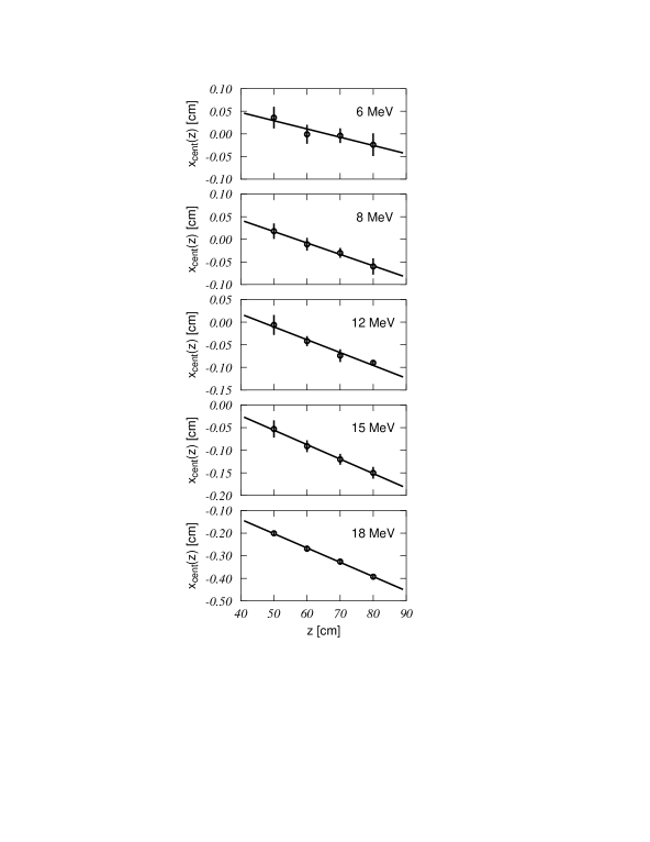
FIG. 2.: Experimental values of $x_{\rm cent}$, obtained in our work, as a function of the distance $z$. The straight lines correspond to the linear regression of the data.

TABLE I.: Results of the fits of the values $\overline{x}_{\rm cent}\pm\sigma_{x_{\rm cent}}$ obtained in our experiment to a linear function of the type $\overline{x}_{\rm cent}\,=\,a\,*\,z\,+\,b$. Note that $b$ defines the position $X_{\rm e}$ of the edge of the collimator.

Energy [MeV]		a		b [cm]		Correlation
6		-0.0017 $\pm$ 0.0009		0.11 $\pm$ 0.06		-0.946
8		-0.0025 $\pm$ 0.0007		0.14 $\pm$ 0.04		-0.997
12		-0.0025 $\pm$ 0.0004		0.11 $\pm$ 0.03		-0.988
15		-0.0032 $\pm$ 0.0006		0.10 $\pm$ 0.04		-0.998
18		-0.0063 $\pm$ 0.0005		0.11 $\pm$ 0.03		-0.999

Once the transverse shifts of the beam edge offset have been measured, we want to check if their variation with $z$ is linear or not. In Table I we give the values of the parameters of the linear regression performed for the experimental centroids. The obtained fits are also shown in Fig. 2 (straight lines). As we can see the correlation coefficients indicate that the way we have introduced in our model the beam divergence is in agreement with the experimental findings, at least in what refers to this aspect of the centroid shift.

Also, it is worth to point out two details concerning the results of this part of the experiment. First, it is satisfactory that the parameter $b$ appears to be constant with the energy. This parameter is measuring (see Eq. (9)) the offset at the collimating plane ($z=0$) and it is obvious that it should be the same in all cases, because the position of the collimator does not change. This is showing again that the procedure of analysis we are carrying out is robust and correct.

Second, the fact that $a$ varies with the energy is due to the differences in the focal spots at the primary foils for each energy. The variation of these focal spots found using the regression we have obtained is of 1.12 mm, which is compatible with the technical specifications of our accelerator.

B Determination of the dose profiles data and their errors

The second point relevant in the experimental part corresponds to the way we have obtained the profiles to be fitted and how the corresponding errors have been estimated.

It is obvious that, due to the character of the process itself, there exists a statistical uncertainty in the dose profiles measured. In order to take care of this point we have measure five new profiles with Setup 3, now with reference chamber, for each energy and for seven values of $z$: 50, 55, 60, 65, 70, 75 and 80 cm. These measurements have been performed together with those used to determine the positions $x_{\rm cent}$, what ensures the validity of the results obtained in the previous subsection to analyze these new profiles. The reason to take these new profiles with the reference chamber (contrary to what we have done for the profiles used to determine the centroid positions) is that it permits a better statistics and a quick procedure, with the obvious beam time saving.

The five dose distributions corresponding to each energy and $z$ are then processed in order to generate the data. First, we have sampled them at different $x$ positions. In this respect it is worth to say that, as we mentioned in Sect. II, we have considered the data obtained below the collimator in order to fulfill the requirement of being at sufficient distance from the physical end of the beam to avoid the possible distortions. Thus, only the values of the dose up to $x=0$ are taken into account. In principle we should have taken into account the doses up to $x_{\rm cent}$ to insure we use only the data in the shadow of the collimator. However, when the profiles were taken the positions of the centroids for the different energies and $z$-values were not known and we sampled up to $x=0$. This means only a few millimeters around the actual values of $x_{\rm cent}$ and we assume this does not invalidate our assumptions. The data obtained in the sampling are averaged to obtain the $\overline{D}(x)$ values at each $x$.

The second step is to estimate the errors accompanying these dose data. To do that we have followed the prescriptions of Ref. [10]. In our case we have two error sources. First, there exists the obvious uncertainty associated to the statistical behavior we have just considered. This kind of error can be evaluated by means of the standard deviation, $\sigma_{D}(x)$, we obtain simultaneously to the mean values $\overline{D}(x)$. This is so because measuring in continuum mode, as we have done, implies the simultaneous consideration of the statistical variation of both the dose and the positioning of the measuring chamber. The corresponding uncertainty is treated as of type A (that is, not assuming an a priori distribution) in the nomenclature of Ref. [10] and then it is evaluated by considering directly the observed distribution. In our case the values found for the relative error corresponding to this statistical spread is below 1% in all cases. (Here the % refers to the relative units in which the profiles are measured).

The second source of error is that linked to the precision of the data acquisition system. This is basically different to the first one and following Ref. [10] is classified as of type B. To evaluate it, we have considered it is the one corresponding to a digital measurement apparatus which is [10]:

$$\Delta_{D}\,=\,\frac{1}{\sqrt{3}}\,\delta_{D}\,=\,0.029\%,$$ (11)

where in our case $\delta_{D}=0.05\%$ is half of the nominal precision of the measurement device.

The total error is then calculated as the quadratic sum of both errors:

$$\Sigma_{D}(x)\,=\,\sqrt{\Delta_{D}^{2}+\sigma_{D}^{2}(x)}\,.$$ (12)

Our data are the relative dose for each energy, $z$ and position $x$, which are given by $\overline{D}(x)\pm\Sigma_{D}(x)$. These values have been fitted as described below.

IV Results

In what follows we discuss the results we have obtained in the analysis of the dose profiles measured as described above.

A Fitting procedure

The dose profiles obtained from our measurements have been fitted using the fitting function in Eq. (10) and by means of the Levenberg-Marquardt method [11]. As indicated in Sect. II, in order to complete the model, we must define the functional dependence of the background function $B(z,x)$ with the position $x$. We have assumed the simplest possibility, that is, the function $B(z,x)$ is constant at each $z$, $B(z,x)\equiv B(z)$. In any case, we have checked that the use of other functional dependences (that is, $B(z,x)$ linear or quadratic, in $x$) does not change the conclusions obtained with respect to the spatial spread.

With our choice for the background function, the fit provides the quantities $D_{\infty}(z)$, $\sigma_{x}(z)$ and $B(z)$ once an input value of $x_{\rm cent}$ is given. In our experiment, $x_{\rm cent}$ was not measured for the intermediate $z$ values 55, 65 and 75 cm. Then, in order to be fully consistent in the fitting procedure, we have used the values of $x_{\rm cent}$ obtained from the linear regression quoted in Table I and shown in Fig. 2. In any case we have checked that same results are obtained in the fits when the experimental $x_{\rm cent}$ values are used in those cases where they are available.

The fact that $D_{\rm fit}$ as given by Eq. (10) is not linear, does not allow an simple analytical estimation of the propagation of the error of $x_{\rm cent}$. Thus, to evaluate the errors corresponding to the three quantities defining our fitting function, we have developed a procedure of Monte Carlo type, which is based on the following steps:

1. From each original profile, we have generated a set of data, which is built by random values normally distributed around the original ones and with standard deviations equal to the associated errors.

2. We have also generated a random value for $x_{\rm cent}$ considering the normal distribution obtained in the linear regression of the experimental values quoted in Subsect. III A.

3. We have fitted the resulting profile with the function (10) again by means of the Levenberg-Marquardt method.

The repetition of this three step procedure provides a set of values for each one of $D_{\infty}(z)$, $\sigma_{x}(z)$ and $B(z)$ and then it is possible to evaluate the corresponding standard deviations for these three quantities. The procedure is repeated until the convergence in the standard deviation values is achieved. We have checked that this happens for a number of random generations between 5000 and 10000. All the results we discuss in the following have been obtained with 10000 generations. The final values found for the standard deviations are taken to be the errors in the three parameters resulting from the fit.

In what follows we discuss the results obtained in the procedure we have followed to fit the relative dose profiles.

B Analysis of $D_{\infty}(z)$

One of the consequences of considering the beam divergence in our model is the fact that the dependence of $D_{\infty}(z)$ with $z$ should follow the inverse square law. In order to check if this is the case, we show in Table II the parameters $a$ and $b$ of the linear regressions $[D_{\infty}(z)]^{-1/2}\,=\,a\,*\,z\,+\,b$ obtained directly from the values of $D_{\infty}(z)$ found in the fitting procedure. As we can see, the data behave as expected (see the correlation factor quoted in the table), what ensures the consistency of the method we have followed. The important point here is that we have not measured directly $D_{\infty}(z)$ but we have used the values obtained from the fit of the tails of the dose profiles below the lead block.

TABLE II.: Results of the linear regression of the values $[D_{\infty}(z)]^{-1/2}$ obtained in our fitting procedure with a fitting function of the type $[D_{\infty}(z)]^{-1/2}\,=\,a\,*\,z\,+\,b$. Also the position of the virtual effective source, $z_{\rm vir}=-b/a$, is given.

Energy [MeV]		a [cm-1]		b		Correlation		$z_{\rm vir}$ [cm]
6		( 8.39 $\pm$ 0.05)$\times 10^{-4}$		(2.09 $\pm$ 0.03)$\times 10^{-2}$		0.99998		-24.8 $\pm$ 0.5
8		( 9.83 $\pm$ 0.05)$\times 10^{-4}$		(2.29 $\pm$ 0.03)$\times 10^{-2}$		0.99968		-23.1 $\pm$ 0.5
12		(10.65 $\pm$ 0.05)$\times 10^{-4}$		(2.42 $\pm$ 0.04)$\times 10^{-2}$		0.99998		-23.2 $\pm$ 0.5
15		(11.22 $\pm$ 0.08)$\times 10^{-4}$		(2.52 $\pm$ 0.05)$\times 10^{-2}$		0.99998		-23.4 $\pm$ 0.7
18		(12.02 $\pm$ 0.10)$\times 10^{-4}$		(2.84 $\pm$ 0.06)$\times 10^{-2}$		0.99998		-23.6 $\pm$ 0.7

One additional point of interest is that these linear regressions allow us to calculate the position of the virtual point source, $z_{\rm vir}=-b/a$. The values obtained are also included in Table II, and, as we can see, the $z_{\rm vir}$ are, for the five energies considered, in a range smaller than 2 cm.

The case of 6 MeV deserve a particular comment. As we can see, the result obtained for this energy is the one showing a larger deviation and, in fact, it differs in 1 cm roughly with respect to the mean of the values of the remaining energies. This is due to the fact that, contrary to what happens for other energies, no primary foil is present in the case of 6 MeV beams. Thus, a shift in $z_{\rm vir}$ of the order of the width of the foil carrier (which is around 1 cm) must be expected in this case. Then, our method is able to reflect in a direct way the architecture of the accelerator head and this shows up again its precision.

In what follows we normalize, for each energy, the dose values to the values $D_{\infty}(z=0)$ obtained from the regressions given in Table II for $[D_{\infty}(z)]^{-1/2}$. This affects the experimental dose data and the values of the parameters $D_{\infty}$ and $B(z)$ shown below. Obviously, the values of $\sigma_{x}(z)$ are not modified by this renormalization.

C Analysis of $B(z)$

The second aspect concerning the results of the fits of the dose profiles we are interested in discussing is the role of the background function $B(z)$. As previously indicated, the reason to include it in our model is to take into account the different scattering processes (part of the dose due to the bremsstrahlung and the dose due to electrons scattered at the gantry head, at the measurement device and its surroundings, as well as those scattered in-air with large angles) which are not described by the pure Gaussian profiles and which, nevertheless, are important to achieve a good description of the experimental data. In Fig. 3 we show the variation with $z$ of the values of $B(z)$ (normalized as indicated above), obtained from the fit, for the five energies we are considering. As we can see, the general trend is, in all cases, to reduce its strength with increasing $z$. This indicates that the electrons scattered in the measuring device seems to be almost negligible because their contribution should be more relevant at large distances, where the bottom of the electro mechanical device for the positioning of the ionization chamber is closer to it. In any case, to establish which scattering mechanism is the main responsible for this background function is not an easy task, mainly because one can expect that, as it occurs for the Gaussian part of the profiles, various processes contribute to this background dose.

Despite the fact that the values of $B(z)$ are small, it is worth to point out that its inclusion in the model is crucial for the good description of the data. This can be seen in Fig. 4, where we show the results obtained for the two extremal energies we consider (6 and 18 MeV) and for the smallest and largest $z$ positions. Therein solid curves correspond to the fits performed with our model, while dashed curves represent the best fits of the data obtained with a pure Gaussian profile (that is with $B(z)=0$ in our model). In both cases the values of $x_{\rm cent}$ obtained experimentally as discussed above have been used. Besides, both calculations, as well as the data, have been normalized to the values $D_{\infty}(z=0)$ obtained within our model. In Table III we give the values found for the parameters in these fits. The first point to note is the goodness of the fits produced by our method. On the other hand, it is worth to point out that the values obtained for the pure Gaussian model differ clearly from those obtained within our approach (including the corresponding uncertainties.)

D Analysis of the spatial spread, $\sigma_{x}(z)$

Our main interest in this work concerns with the determination of the spatial spread of clinical electron beams in order to characterize them. In our model, the spatial spread determined in the fitting procedure corresponds to the Gaussian part of the dose profiles measured. According to Fermi-Eyges theory, this spatial spread must show a quadratic-cubic dependence with $z$. In particular, this dependence is given by (see e.g. Ref. [5]):

$$\sigma_{x}^{2}(z)\,=\,\sigma_{\theta,{\rm i}}^{2}\,z^{2}\,+\,\frac{1}{6}\,T(E)\,z^{3}\,,$$ (13)

where $\sigma_{\theta,{\rm i}}^{2}$ is the initial quadratic angular spread and $T(E)$ is the air linear scattering power corresponding to the energy $E$ and we assume it to be independent of $z$. Both parameters can be found by fitting with Eq. (13) the $\sigma_{x}(z)$ values obtained from the fitting of the dose profiles. Instead of doing directly this, and in order to simplify the analysis, we have linearly regressed the quantity $\sigma_{x}^{2}(z)/z^{2}$ as a function of $z$. The values obtained are given in Table IV. The regression lines we have found in this procedure are plotted in Fig. 5 with full lines. It is apparent the good agreement produced in this case with the experimental data, what guarantees the feasibility of the previous assumption concerning the significance of the spatial spread we have determined.

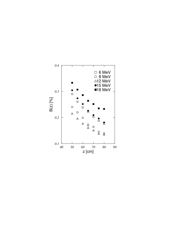
FIG. 3.: Values of $B(z)$ obtained in the fitting procedure and normalized to $D_{\infty}(z=0)$ as described in the text.

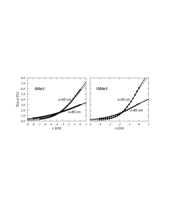
FIG. 4.: Experimental dose profiles for 6 (upper panel) and 18 MeV (lower panel). Solid curves have been obtained by fitting the experimental doses with the function of Eq. (10). Dashed lines correspond to the best fits obtained with pure Gaussian profiles ($B(z)=0$). The values of the parameters $D_{\infty}(z)$, $\sigma_{x}(z)$ and $B(z)$ found in both fits are given in Table III. In both cases the experimental values of $x_{\rm cent}$ have been considered. At the scale of the figure, the errors bars are smaller than the symbols used to represent the data. The normalization to $D_{\infty}(z=0)$ as described in the text is included.

TABLE III.: Values of the parameters $D_{\infty}(z)$, $\sigma_{x}(z)$ and $B(z)$ obtained in the fits of the experimental dose profiles measured for the extremal energies considered in our work (6 and 18 MeV) and the shortest and largest distances to the source (50 and 80 cm). The values quoted as “Our model” have been found with Eq. (10), while in those quoted as “Pure Gaussian” the background function $B(z)$ has been taken to be zero. The values of $D_{\infty}(z)$, for both models, and $B(z)$ are normalized as described in the text.

			“Our model”						“Pure Gaussian”
Nominal Energy	$z$		$D_{\infty}(z)$		$\sigma_{x}(z)$		$B(z)$		$D_{\infty}(z)$	$\sigma_{x}(z)$
[MeV]	[cm]		[%]		[cm]		[%]		[%]	[cm]
6	50		11.08$\pm$0.05		2.99$\pm$0.01		0.289$\pm$0.003		11.01	3.5
	80		5.65$\pm$0.02		5.19$\pm$0.02		0.171$\pm$0.007		5.87	5.7
18	50		10.31$\pm$0.07		1.30$\pm$0.01		0.325$\pm$0.002		10.64	1.5
	80		5.20$\pm$0.02		2.12$\pm$0.01		0.222$\pm$0.06		5.59	2.4

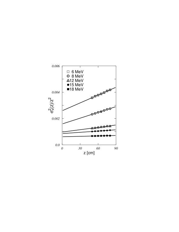
FIG. 5.: Values of $\sigma_{x}^{2}(z)/z^{2}$ obtained in the fitting procedure of the dose profiles. Full lines correspond to the fits performed with the function of Eq. (13). The error bars are smaller than the width of the symbols used.

Scattering powers are important because they permit to find the angular spread at any $z$. In fact, $\sigma_{\theta}^{2}(z)$ behaves linearly with $z$ and the slope is precisely $T(E)$. Then it is relevant to compare the values obtained in our approach with those given in other references. To do that the first point to elucidate is to fix the beam energy at which the scattering power is determined. The beam energies we have quoted up to now are actually the nominal ones. To calculate $T(E)$ we have used, instead, the mean beam energies at the isocenter. Following the prescription of Ref. [5], these energies have been obtained from the equation $\overline{E}_{0}\,=\,C_{6}\,R_{50}$, where $C_{6}=2.33$ MeV/cm. The parameter $R_{50}$ is the half-value depth, which is determined by range measurements in water at SSD=100 cm and with broad beam. The values obtained, $\overline{E}_{0}$, are also given in Table IV. With these values of the mean energies corresponding to our beam, we have calculated the values of $T(E)$ by interpolating those quoted in Table 2.6 of Ref. [5] and correcting them for Møller scattering.

As one can see, these values differ from those obtained with our model by a factor $\sim 2$ or even bigger. In principle, this means that the lineal scattering powers we have found suggest energies for the beam considerably bigger than the mean energies determined experimentally as mentioned above. However one should be careful with the interpretation of these results because of the approach considered in Ref. [5] to obtain the $T(E)$ values is quite different from ours. In this sense, a more detailed investigation in this direction is needed before establishing definitive conclusions. The possibilities open by the results we have obtained with our method are especially interesting in this respect due to its simplicity and accuracy.

TABLE IV.: Values of $\sigma_{\theta,{\rm i}}^{2}$ and $T(E)$ obtained with our model, mean beam energies at the isocenter $\overline{E}_{0}$ (see text) and $T(E)$ values found by interpolating those given in Table 2.6 of Ref. [5] for these mean energies and corrected for Møller scattering.

		“Our model”						Ref. [5]
Nominal Energy		$\sigma_{\theta,{\rm i}}^{2}$		$T(E)$		$\overline{E}_{0}$		$T(\overline{E}_{0})$
[MeV]		[rad2]		[rad2 cm-1]		[MeV]		[rad2 cm-1]
6		$(25.5\pm 0.6)\times 10^{-4}$		$(12.5\pm 0.6)\times 10^{-5}$		5.3		$24.983\times 10^{-5}$
8		$(16.2\pm 0.4)\times 10^{-4}$		$(~{}8.8\pm 0.3)\times 10^{-5}$		7.2		$14.663\times 10^{-5}$
12		$(10.1\pm 0.2)\times 10^{-4}$		$(~{}3.3\pm 0.2)\times 10^{-5}$		11.0		$~{}7.015\times 10^{-5}$
15		$(~{}8.9\pm 0.2)\times 10^{-4}$		$(~{}1.6\pm 0.2)\times 10^{-5}$		13.9		$~{}4.670\times 10^{-5}$
18		$(~{}6.2\pm 0.2)\times 10^{-4}$		$(~{}0.6\pm 0.1)\times 10^{-5}$		16.9		$~{}3.324\times 10^{-5}$

V Summary and conclusions

In this work we have proposed, developed and tested a new procedure to determine the spatial spread of clinical electron beams. Two are the main advantages of the method proposed. First, we have assumed that the dose profiles can be described by means of a function which includes both a Gaussian part and a background function, this last taking into account those processes not considered in the first one. Second, this new method is based on the direct fit of the dose profiles measured at the center of the beam and below a lead block covering half of the beam. The beam divergence is incorporated to the model in a very easy way and its consequences (the inverse squared law and the linear shift of the centroid) are checked to be fulfilled with a high accuracy. Besides, the fitting procedure provides the spatial spread in a straightforward way and a great part of the ambiguities and errors of the usual methods based in penumbra measurements are eliminated.

The data obtained in this way for the spatial spread have been fitted to a quadratic-cubic function of the distance $z$. The nice fits obtained confirm the behavior expected from the Fermi-Eyges theory for the Gaussian part of our model and open the possibility for using our approach to measure the scattering power in air.

We think that the model we propose in this work deserves a more detailed study because of its possible application to describe the clinical electron beam behavior. Obviously, it is necessary to apply it to a variety of different measuring circumstances in order to complete its validity for this purpose. Thus, it is mandatory to proceed with the applicator, what will provide us information clinically relevant. Also, the results obtained with phantoms of, e.g., water will permit to elucidate the accuracy of our procedure for more practical situations. Work in these directions is in progress.

REFERENCES

- [1] K.R. Hogstrom, M.D. Mills, and P.R. Almond, Phys. Med. Biol. 26, 445 (1981).
- [2] H. Huizenga and P.R.M. Storchi, Phys. Med. Biol. 32, 1011 (1987).
- [3] G.A. Sandison and W. Huda, Med. Phys. 15, 498 (1988).
- [4] P.J. Keall and P.W. Hoban, Phys. Med. Biol. 41, 1511 (1996).
- [5] ICRU Report No. 35, “Radiation Dosimetry: Electron Beams with Energies Between 1 and 50 MeV,” (Bethesda, 1984).
- [6] J.C. Zapata, M. Vilches, D. Guirado, D. Fernández, and A.M. Lallena, (in preparation).
- [7] A.L. McKenzie, Phys. Med. Biol. 24, 628 (1979).
- [8] B.L. Werner, F.M. Khan, and F.C. Deibel, Med. Phys. 9, 180 (1982).
- [9] M. Abramowitz and I. A. Stegun, “Handbook of Mathematical Functions,” (Dover Publications, Inc., New York, 1972).
- [10] ISO/TAG 4 Work Group 3, “Guide to the Expressions of Uncertainties in Measurements”, (ISO, Genève, 1992)
- [11] W.H. Press, S.A. Teukolsky, W.T. Vetterling and B.P. Flannery, “Numerical Recipes in Fortran. The Art of Scientific Computing, 2nd. Ed.”, (Cambridge University Press, Cambridge, 1992)