Collective Motion

Abstract

With the aim of understanding the emergence of collective motion from local interactions of organisms in a ”noisy” environment, we study biologically inspired, inherently non-equilibrium models consisting of self-propelled particles. In these models particles interact with their neighbors by turning towards the local average direction of motion. In the limit of vanishing velocities this behavior results in a dynamics analogous to some Monte Carlo realization of equilibrium ferromagnets. However, numerical simulations indicate the existence of new types of phase transitions which are not present in the corresponding ferromagnets. In particular, here we demonstrate both numerically and analytically that even in certain one dimensional self-propelled particle systems an ordered phase exists for finite noise levels.

1 Introduction

The collective motion of organisms (flocking of birds, for example), is a fascinating phenomenon capturing our eyes when we observe our natural environment. In addition to the aesthetic aspects, studies on collective motion can have interesting applications as well: a better understanding of the swimming patterns of large schools of fish can be useful in the context of large scale fishing strategies, or modeling the motion of a crowd of people can help urban designers. Here we address the question whether there are some global, perhaps universal features of this type of behavior when many organisms are involved and such parameters as the level of perturbations or the mean distance between the organisms is changed.

Our interest is also motivated by the recent developments in areas related to statistical physics. During the last 15 years or so there has been an increasing interest in the studies of far-from-equilibrium systems typical in our natural and social environment. Concepts originated from the physics of phase transitions in equilibrium systems [1] such as collective behavior, scale invariance and renormalization have been shown to be useful in the understanding of various non-equilibrium systems as well. Simple algorithmic models have been helpful in the extraction of the basic properties of various far-from-equilibrium phenomena, like diffusion limited growth [2], self-organized criticality [3] or surface roughening [4]. Motion and related transport phenomena represent a further characteristic aspect of non-equilibrium processes, including traffic models [5], thermal ratchets [6] or driven granular materials [7].

Self-propulsion is an essential feature of most living systems. In addition, the motion of the organisms is usually controlled by interactions with other organisms in their neighborhood and randomness also plays an important role. In Ref. [8] a simple model of self propelled particles (SPP) was introduced capturing these features with a view toward modeling the collective motion [9, 10] of large groups of organisms such as schools of fish, herds of quadrupeds, flocks of birds, or groups of migrating bacteria [11, 12, 13, 14, 15], correlated motion of ants [16] or pedestrians [17]. Our original SPP model represents a statistical physics-like approach to collective biological motion complementing models which take into account much more details of the actual behavior of the organism [9, 18], but, as a consequence, treat only a moderate number of organisms and concentrate less on the large scale behavior.

In spite of the analogies with ferromagnetic models, the general behavior of SSP systems are quite different from those observed in equilibrium models. In particular, in the case of equilibrium ferromagnets possessing continuous rotational symmetry the ordered phase is destroyed at finite temperatures in two dimensions [19]. However, in the 2d version of the SSP model phase transitions can exist at finite noise levels (temperatures) as it was demonstrated by simulations [8, 20] and by a theory of flocking developed by Toner and Tu [21] based on a continuum equation proposed by them. Further studies showed that modeling collective motion leads to similar interesting specific results in all of the relevant dimensions (from 1 to 3). Therefore, after introducing the basic version of the model (in 2d) we discuss the results for each dimension separately and then focus on the 1d case which is better accessible for theoretical analysis.

2 A generic model of two dimensional SPP system

The model consists of particles moving on a plane with periodic boundary condition. The particles are characterized by their (off-lattice) location $\vec{x}_{i}$ and velocity $\vec{v}_{i}$ pointing in the direction $\vartheta_{i}$. To account for the self-propelled nature of the particles the magnitude of the velocity is fixed to $v_{0}$. A simple local interaction is defined in the model: at each time step a given particle assumes the average direction of motion of the particles in its local neighborhood $S(i)$ with some uncertainty, as described by

$$\vartheta_{i}(t+\Delta t)=\langle\vartheta(t)\rangle_{S(i)}+\xi,$$ (1)

where the noise $\xi$ is a random variable with a uniform distribution in the interval $[-\eta/2,\eta/2]$. The locations of the particles are updated as

$$\vec{x}_{i}(t+\Delta t)=\vec{x}_{i}(t)+\vec{v}_{i}(t)\Delta t.$$ (2)

The model defined by Eqs. (1) and (2) is a transport related, non-equilibrium analog of the ferromagnetic models [22]. The analogy is as follows: the Hamiltonian tending to align the spins in the same direction in the case of equilibrium ferromagnets is replaced by the rule of aligning the direction of motion of particles, and the amplitude of the random perturbations can be considered proportional to the temperature for $\eta\ll 1$. From a hydrodynamical point of view, in SPP systems the momentum of the particles is not conserved. Thus, the flow field emerging in these models can considerably differ from the usual behavior of fluids.

3 Collective motion

The model defined through Eqs. (1) and (2) was studied by performing large-scale Monte-Carlo simulations in Ref. [20]. Due to the simplicity of the model, only two control parameter should be distinguished: the (average) density of particles $\varrho$ and the amplitude of the noise $\eta$.

For the statistical characterization of the configurations, a well-suited order parameter is the magnitude of the average momentum of the system: $\phi\equiv\left|\sum_{j}\vec{v}_{j}\right|/N$. This measure of the net flow is non-zero in the ordered phase, and vanishes (for an infinite system) in the disordered phase.

Since the simulations were started from a disordered configuration, $\phi(t=0)\approx 0$. After some relaxation time a steady state emerges indicated, e.g., by the convergence of the cumulative average $(1/\tau)\int^{\tau}_{0}\phi(t)dt$. The stationary values of $\phi$ are plotted in Fig. 1a vs $\eta$ for $\varrho=2$ and various system sizes $L$. For weak noise the model displays long-range ordered motion (up to the actual system size $L$, see Fig.2), that disappears in a continuous manner by increasing $\eta$.

As $L\rightarrow\infty$, the numerical results show the presence of a kinetic phase transition described by

$$\phi(\eta)\sim\cases{\Bigl{(}{\eta_{c}(\varrho)-\eta\over\eta_{c}(\varrho)}\Bigr{)}^{\beta}&for $\eta<\eta_{c}(\varrho)$\cr 0&for $\eta>\eta_{c}(\varrho)$\cr},$$ (3)

where $\eta_{c}(\varrho)$ is the critical noise amplitude that separates the ordered and disordered phases and $\beta=0.42\pm 0.03$, found to be different from the the mean-field value $1/2$ (Fig 1b).

Figure 1: (a) The average momentum of the 2D SPP model in the steady state vs the noise amplitude $\eta$ for $\varrho=2$ and four different system sizes [($\diamond$) $N=800$, $L=20$; ($+$) $N=3200$, $L=40$; ($\Box$) $N=20000$, $L=100$ and ($\times$) $N=10^{5}$, $L=223$]. (b) The order present at small $\eta$ disappears in a continuous manner reminiscent of second order phase transitions: $\phi\sim[(\eta_{c}(L)-\eta)/\eta_{c}(L)]^{\beta}\equiv(\Delta\eta/\eta_{c})^{\beta}$, with $\beta=0.42$, different from the mean-field value $1/2$ (solid line).

Figure 2: The velocities of the SPPs are displayed for various values of density and noise. The actual velocity of a particle is indicated by a small arrow, while its trajectory for the last 20 time step is shown by a short continuous curve. For comparison, the range of the interaction is displayed as a bar. (a) At high densities and small noise ($N=300$, $L=5$ and $\eta=0.1$) the motion becomes ordered. (b) For small densities and noise ($N=300$, $L=25$ and $\eta=0.1$) the particles tend to form groups moving coherently in random directions.

In an analogy with equilibrium phase transitions, singular behavior of the order parameter as a function of the density and critical scaling of the fluctuations of $\phi$ was also observed. These results can be summarized as

$$\phi(\eta,\varrho)=\tilde{\phi}\bigl{(}\eta/\eta_{c}(\varrho)\bigr{)},$$ (4)

where $\tilde{\phi}(x)\sim(1-x)^{\beta}$ for $x<1$, and $\tilde{\phi}(x)\approx 0$ for $x>1$. The critical line $\eta_{c}(\varrho)$ in the $\eta-\varrho$ parameter space was found to follow

$$\eta_{c}(\varrho)\sim\varrho^{\kappa},$$ (5)

with $\kappa=0.45\pm 0.05$. Eq.(4) also implies that the exponent $\beta^{\prime}$, defined as $\phi\sim(\varrho-\varrho_{c})^{\beta^{\prime}}$ for $\varrho>\varrho_{c}$ [8], must be equal to $\beta$. The standard deviation ($\sigma$) of the order parameter behaved as

$$\sigma(\eta)\sim|\eta-\eta_{c}|^{-\gamma},$$ (6)

with an exponent $\gamma$ close to $2$, which value is, again, different from the mean-field result.

These findings indicate that the SPP systems can be quite well characterized using the framework of classical critical phenomena, but also show surprising features when compared to the analogous equilibrium systems. The velocity $v_{0}$ provides a control parameter which switches between the SPP behavior ($v_{0}>0$) and an $XY$ ferromagnet ($v_{0}=0$). Indeed, for $v_{0}=0$ Kosterlitz-Thouless vortices [23] could be observed in the system, which turned out to be unstable for any nonzero $v_{0}$ investigated in [20].

4 Phase diagram for a 3d SPP system

In two dimensions an effective long range interaction can build up because the migrating particles have a condiderably higher chance to get close to each other and interact than in three dimensions (where, as is well known, random trajectories do not overlap). The less interaction acts against ordering. On the other hand, in three dimensions even regular ferromagnets order. Thus, it is interesting to see how these two competing features change the behavior of 3d SPP systems. The convenient generalization of Eq. (1) for the 3d case can be the following [24]:

$$\vec{v}_{i}(t+\Delta t)=v_{0}\hbox{ \bf N}(\hbox{ \bf N}(\langle\vec{v}(t)\rangle_{S(i)})+\vec{\xi}),\\$$ (7)

where $\hbox{ \bf N}(\vec{u})=\vec{u}/|\vec{u}|$ and the noise $\vec{\xi}$ is uniformly distributed in a sphere of radius $\eta$.

Generally, the behavior of the system was found [24] to be similar to that of described in the previous section. The long-range ordered phase was present for any $\varrho$, but for a fixed value of $\eta$, $\phi$ vanished with decreasing $\varrho$. To compare this behavior to the corresponding diluted ferromagnet, $\phi(\eta,\varrho)$ was determined for $v_{0}=0$, when the model reduces to an equilibrium system of randomly distributed ”spins” with a ferromagnetic-like interaction. Again, a major difference was found between the SPP and the equilibrium models (Fig. 3): in the static case the system does not order for densities below a critical value close to 1 which corresponds to the percolation threshold of randomly distributed spheres in 3d.

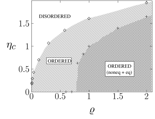
Figure 3: Phase diagram of the 3d SPP and the corresponding ferromagnetic system. The diamonds show our estimates for the critical noise for a given density for the SPP model and the crosses show the same for the static case. The SPP system becomes ordered in the whole region below the curved line connecting the diamonds, while in the static case the ordered region extends only down to the percolation threshold $\rho\simeq 1$.

5 Ordered motion for finite noise in 1d

In order to study the 1d SPP model a few changes in the updating rules had to be introduced. Since in 1d the particles cannot get around each other, some of the interesting features of the dynamics are lost (and the original version would become a trivial cellular automaton type model). However, if the algorithm is modified to take into account the specific crowding effects typical for 1d (the particles can slow down before changing direction and dense regions may be built up of momentarily oppositely moving particles) the model becomes more realistic.

Thus, in [25] $N$ off-lattice particles along a line of length $L$ has been considered. The particles are characterized by their coordinate $x_{i}$ and dimensionless velocity $u_{i}$ updated as

$$x_{i}(t+\Delta t)=x_{i}(t)+v_{0}u_{i}(t)\Delta t,$$ (8)

$$u_{i}(t+\Delta t)=G\Bigl{(}\langle u(t)\rangle_{S(i)}\Bigr{)}+\xi_{i}.$$ (9)

The local average velocity $\langle u\rangle_{S(i)}$ for the $i$th particle is calculated over the particles located in the interval $[x_{i}-\Delta,x_{i}+\Delta]$, where we fix $\Delta=1$. The function $G$ incorporates both the propulsion and friction forces which set the velocity in average to a prescribed value $v_{0}$: $G(u)>u$ for $u<1$ and $G(u)<u$ for $u>1$. In the numerical simulations [25] one of the simplest choices for $G$ was implemented as

$$G(u)=\cases{(u+1)/2&for $u>0$\cr(u-1)/2&for $u<0$,\cr}$$ (10)

and random initial and periodic boundary conditions were applied.

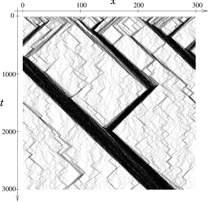
Figure 4: The first 3000 time steps of the 1d SPP model [$L=300$, $N=600$, $\eta=2.0$ (a) and $\eta=4.0$ (b)]. The darker gray scale represents higher particle density.

Figure 5: Phase diagram in the $\rho-\eta$ plane, the critical line follows $\eta_{c}(\rho)\sim\rho^{\kappa}$. The solid curve represents a fit with $\kappa=1/4$.

In Fig. 4 we show the time evolution of the model for $\eta=2.0$. In a short time the system reaches an ordered state, characterized by a spontaneous broken symmetry and clustering of the particles. In contrast, for $\eta=4.0$ the system would remain in a disordered state. The $\rho-\eta$ phase diagram is shown in Fig. 5. The critical line, $\eta_{c}(\varrho)$, follows (5) with $\kappa\approx 1/4$.

6 Analytical studies of SPP systems

To understand the phase transitions observed in the models described in the previous section, efforts has been made to set up a consistent continuum theory in terms of $\vec{v}$ and $\rho$, representing the coarse-grained velocity and density fields, respectively. The first approach [21] has been made by J. Toner and Y. Tu who investigated the following set of equations

$$\partial_{t}\vec{v}+(\vec{v}\nabla)\vec{v} = \alpha\vec{v}-\beta|\vec{v}|^{2}\vec{v}-\nabla P+D_{L}\nabla(\nabla\vec{v})+D_{1}\nabla^{2}\vec{v}+D_{2}(\vec{v}\nabla)^{2}\vec{v}+\xi$$

$$\partial_{t}\rho+\nabla(\rho\vec{v}) = 0,$$ (11)

where the $\alpha,\beta>0$ terms make $\vec{v}$ have a nonzero magnitude, $D_{L,1,2}$ are diffusion constants and $\xi$ is an uncorrelated Gaussian random noise. The pressure $P$ depends on the local density only, as given by the expansion

$$P(\rho)=\sum_{n}\sigma_{n}(\rho-\rho_{0})^{n}.$$ (12)

The non-intuitive terms in Eq.(11) were generated by the renormalization process.

Tu and Toner were able to treat the problem analytically and show the existence of an ordered phase in 2d, and also extracted exponents characterizing the density-density correlation function. They showed that the upper critical dimension for their model is 4, and the theory does not allow an ordered phase in 1d.

However, as we have shown in the previous section, there exist SPP systems in one dimension which exhibit an ordered phase for low noise level. Such systems can not belong to the universality class investigated in [21]. This finding motivated the construction of an other continuum model, which can be derived from the master equation of the 1d SPP system [25]:

$$\partial_{t}U = f(U)+\mu^{2}\partial_{x}^{2}U+\alpha{(\partial_{x}U)(\partial_{x}\rho)\over\rho}+\zeta,$$ (13)

$$\partial_{t}\rho = -v_{0}\partial_{x}(\rho U)+D\partial_{x}^{2}\rho,$$ (14)

where $U(x,t)$ is the coarse-grained dimensionless velocity field, the self-propulsion term, $f(U)$, is an antisymmetric function with $f(U)>0$ for $0<U<1$ and $f(U)<0$ for $U>1$. The noise, $\zeta$, has zero mean and a density-dependent standard deviation: $\overline{\zeta^{2}}=\sigma^{2}/\rho\tau^{2}$. These equations are different both from the equilibrium field theories and from the nonequilibrium system defined through Eqs(11). The main difference comes from the nature of the coupling term $(\partial_{x}U)(\partial_{x}\rho)/\rho$ which can be derived from the microscopic alignment rule (1) [26]. Note, that the noise also has different statistical properties from the one considered in (11). For $\alpha=0$ the dynamics of the velocity field $U$ is independent of $\rho$ and with an appropriate choice of $f$ Eq.(13) becomes equivalent to the $\Phi^{4}$ model describing spin chains, where domains of opposite magnetization develop at finite temperatures [1].

7 Linear Stability Analysis

To study the effect of the nonlinear coupling term $\alpha{(\partial_{x}U)(\partial_{x}\rho)/\rho}$, we now investigate the development of the ordered phase in the deterministic case ($\sigma=0$) when $c,D\ll 1$ holds. It can be seen that stationary domain wall solutions exist for any $\alpha$. In particular, let us denote by $\rho^{*}$ and $U^{*}$ the stationary solutions which satisfy $\rho^{*}(\pm\infty)=0$, $U^{*}(\pm\infty)=\mp 1$, $U^{*}(x)<0$ for $x>0$ and $U^{*}(x)>0$ for $x<0$. These functions are determined as

$$\ln{\rho^{*}(x)\over\rho^{*}(0)}={c\over D}\int_{0}^{x}U^{*}(x^{\prime})dx^{\prime}$$ (15)

and

$$\mu^{2}\partial_{x}^{2}U^{*}=-f(U^{*})-\alpha{c\over D}U^{*}\partial_{x}U^{*}.$$ (16)

Although stationary solutions exist for any $\alpha$, they are not always stable against long wavelength perturbations, as the following linear stability analysis shows.

Let us assume that at $t=0$ we superimpose an $u(x,t=0)$ perturbation over the $U^{*}(x)$ stationary solution. Since $c,D\ll 1$ the dynamics of $\rho$ is slow, thus $\rho(x,t)=\rho^{*}(x)$ is assumed. The stationary solutions are metastable in the sense that small perturbations can transform them into equivalent, shifted solutions. Thus here by linear stability or instability we mean the existence or inexistence of a stationary solution to which the system converges during the response to a small perturbation. To handle the set of possible metastable solutions we write the perturbation $u$ in the form of $\tilde{u}$ as

$$U(x,t)=U^{*}(x)+u(x,t)=U^{*}(x-\xi(t))+\tilde{u}(x,t),$$ (17)

i.e.,

$$\tilde{u}(x,t)=u(x,t)+\xi(t)a(x),$$ (18)

where $a\leq 0$ denotes $\partial_{x}U^{*}$ and the position of the domain wall, $\xi(t)$, is defined by the implicit

$$U(\xi(t),t)=0$$ (19)

equation. As $U^{*}(0)=0$, from (19) we have $\tilde{u}(\xi,t)=0$. The usage of $\xi$ and $\tilde{u}$ is convenient, since the stability of the stationary solution $U^{*}$ is equivalent with the convergence of $\xi(t)$ as $t\rightarrow\infty$.

Substituting (17) into (14) and taking into account the stationarity of $U^{*}$ we get

$$-a(x-\xi)\dot{\xi}+\partial_{t}\tilde{u}(x)=(f^{\prime}\circ U^{*})(x-\xi)\tilde{u}(x)+\mu^{2}\partial_{x}^{2}\tilde{u}(x)+\alpha\xi h(x-\xi),$$ (20)

with $h=a\partial_{x}^{2}\ln\rho^{*}\geq 0$. To simplify Eq.(20 let us write $(f^{\prime}\circ U^{*})(x)$ in the form of $g(x)-g_{\infty}$, where $g_{\infty}=-lim_{x\rightarrow\pm\infty}f^{\prime}(U^{*}(x))=-f^{\prime}(\pm 1)$. Furthermore, a moving frame of reference $y=x-\xi$ and the new variable $v(y)=u(x)$ can be defined. With these new notations Eq.(20) becomes

$$-a(y)\dot{\xi}+\partial_{t}v(y)=g(y)v(y)-g_{\infty}v(y)+\mu^{2}\partial_{x}^{2}v(y)+\alpha\xi h(y).$$ (21)

The time development of $\xi$ is determined by the $u(\xi)=v(0)=0$ condition yielding

$$-a(0)\dot{\xi}=\mu^{2}\partial_{x}^{2}v(0)+\alpha\xi h(0).$$ (22)

By the Fourier-transformation of Eq. (21), treating the gv term as a perturbation, for the time derivatives of $\xi(t)$ and the $n$-th Fourier moments $\hat{v}_{n}(t)\sim\partial_{x}^{n}v(0,t)$ one can obtain [27]

$${d\over dt}\pmatrix{-\hat{a}_{0}&&&\cr-\hat{a}_{2}&1&&\cr-\hat{a}_{4}&&1&\cr\vdots&&&\ddots\cr}\pmatrix{\xi\cr\hat{v}_{2}\cr\hat{v}_{4}\cr\vdots}=\pmatrix{\alpha\hat{h}_{0}&-\mu^{2}&&\cr\alpha\hat{h}_{2}&-g_{\infty}&-\mu^{2}&\cr\alpha\hat{h}_{4}&&-g_{\infty}&-\mu^{2}\cr\vdots&&&\ddots\cr}\pmatrix{\xi\cr\hat{v}_{2}\cr\hat{v}_{4}\cr\vdots}.$$ (23)

Expression (23) can be further simplified using the relations $\hat{a}_{m}\ll\hat{a}_{n}$ and $\hat{h}_{m}\ll\hat{h}_{n}$ for $m>n$ and the approximate solutions for the $\lambda$ growth rate of the original $u$ perturbation we found [27]

$$\lambda_{0}=\hat{a}_{0}g_{\infty}<0$$ (24)

and $\lambda_{+}$,$\lambda_{-}$ satisfying

$$\lambda_{\pm}^{2}-b\lambda_{\pm}+q=0,$$ (25)

where

$$b = \alpha\hat{h}_{0}-\mu^{2}\hat{a}_{2}+g_{\infty}\hat{a}_{0},$$ (26)

$$q = \alpha\hat{a}_{0}(\hat{h}_{0}g_{\infty}-\hat{h}_{2}\mu^{2}).$$ (27)

If $\alpha=0$, then $\lambda_{+}=0$ and $\lambda_{-}=g_{\infty}\hat{a}_{0}-\mu^{2}\hat{a}_{2}<0$. However, for certain $\alpha>0$ values $\lambda_{+}>0$ can hold obtained as either $q<0$ or $b>0$, i.e.,

$$\alpha>\alpha_{c,1}=D{3g_{\infty}-2g(0)\over 2ca(0)}$$ (28)

or

$$\alpha>\alpha_{c,2}=D{2g_{\infty}-g(0)\over a(0)(c-D)},$$ (29)

respectively. Thus for $\alpha>\alpha_{c}=min(\alpha_{c,1},\alpha_{c,2})$ the stability of the domain wall solution disappears.

The instability of the domain wall solutions gives rise to the ordering of the system as the following simplified picture shows. A small domain of (left moving) particles moving opposite to the surrounding (right moving) ones is bound to interact with more and more right moving particles and, as a result, the domain wall assumes a specific structure which is characterized by a buildup of the right moving particles on its left side, while no more than the originally present left moving particles remain on the right side of the domain wall. This process ”transforms” non-local information (the size of the corresponding domains) into a local asymmetry of the particle density which, through the instability of the walls, results in a leftward motion of the domain wall, and consequently, eliminates the smaller domain.

This can be demonstrated schematically as

• $>>>>>>>>>>><<<<<<<<>>>>>>>>>>>>>$

• $~{}~{}~{}~{}~{}~{}~{}~{}~{}~{}~{}~{}~{}~{}~{}~{}~{}~{}~{}~{}~{}~{}~{}~{}~{}A~{}~{}~{}~{}~{}~{}~{}~{}~{}~{}~{}~{}~{}~{}~{}~{}~{}B$

where by $>(<)$ we denoted the right (left) moving particles. In contrast to the Ising model the $A$ and $B$ walls are very different and have nonequivalent properties. In this situation the $B$ wall will break into a $B_{1}$ and $B_{2}$, moving in opposite directions, $B_{1}$ moving to the left and $B_{2}$ moving to the right, leaving the area $B_{1}-B_{2}$ behind, which is depleted of particles.

• $>>>>>>>>>>><<<<<~{}~{}~{}~{}~{}~{}~{}~{}~{}~{}~{}~{}>>>>>>>>>>$

• $~{}~{}~{}~{}~{}~{}~{}~{}~{}~{}~{}~{}~{}~{}~{}~{}~{}~{}~{}~{}~{}~{}~{}~{}~{}A~{}~{}~{}~{}~{}~{}~{}B_{1}~{}~{}~{}~{}~{}~{}~{}~{}~{}B_{2}$

At the $A$ boundary the two type of particles slow down, while, due to the instability we showed to be present in the system, the wall itself moves in a certain direction, most probably to the right. Even in the other, extremely rare case (i.e., when the $A$ wall moves to the left), an elimination of the smaller domain ($A-B_{1}$) takes place since the velocity of the domain wall $A$ is smaller than the velocity of the particles in the ”bulk” and at $B_{1}$ where the local average velocity is the same as the preferred velocity of the particles. Thus, the particles tend to accumulate at the domain wall $A$, which again, through local interactions leads to the elimination of the domain $A-B_{1}$.

It is easy to see that the $U=\pm 1$ solutions are absolute stable against small perturbations, thus it is plausible to assume that the system converges into those solutions even for finite noise.

References

- 1. S.-K. Ma, Statistical Mechanics (World Scientific, Singapore, 1985); Modern Theory of Critical Phenomena (Benjamin, New York, 1976); H. E. Stanley, Introduction to Phase Transitions and Critical Phenomena (Oxford University Press, Oxford, 1971).
- 2. T. A. Witten and L. M. Sander, Phys. Rev. Lett. 47, 1400 (1981); T. Vicsek, Fractal Growth Phenomena, Second Edition (World Scientific, Singapore, 1992).
- 3. P. Bak, C. Tang and K. Wiesenfeld, Phys. Rev. Lett. 59, 381 (1987).
- 4. A-L. Barabási and H. E. Stanley, Fractal Concepts in Surface Growth (Cambridge University Press, Cambridge, 1995)
- 5. See, e.g., K. Nagel, Phys Rev E 53, 4655 (1996), and references therein
- 6. M. O. Magnasco, Phys. Rev. Lett. 71, 1477 (1993);
- 7. Y. L. Duparcmeur, H.J. Herrmann and J. P. Troadec, J. Phys. (France) I, 5, 1119 (1995); J. Hemmingsson, J. Phys. A 28, 4245 (1995).
- 8. T. Vicsek, A. Czirók, E. Ben-Jacob, I. Cohen and O. Shochet, Phys. Rev. Lett. 75, 1226 (1995).
- 9. C. W. Reynolds, Computer Graphics 21, 25 (1987).
- 10. D. P. O’Brien J. Exp. Mar. Biol. Ecol. 128, 1 (1989); J. L. Deneubourg and S. Goss, Ethology, Ecology, Evolution 1, 295 (1989); A. Huth and C. Wissel, in Biological Motion, eds. W. Alt and E. Hoffmann (Springer Verlag, Berlin, 1990).
- 11. C. Allison and C. Hughes, Sci. Progress 75, 403 (1991);
- 12. J.A. Shapiro, Sci. Amer. 256, 82 (1988); E.O. Budrene and H.C. Berg, Nature 376, 49 (1995)
- 13. H. Fujikawa and M.Matsushita, J. Phys. Soc. Jap. 58, 3875 (1989); (1994); E. Ben-Jacob, I. Cohen, O. Shochet, A. Tenenbaum, A. Czirók,and T. Vicsek, Nature 368, 46 (1994); Phys. Rev. Lett. 75, 2899 (1995).
- 14. A. Czirók, E. Ben-Jacob, I. Cohen and T. Vicsek, Phys. Rev. E 54, 1791 (1996).
- 15. G. Wolf, (ed.). Encyclopaedia Cinematographica: Microbiology. Institut für den Wissenschaftlichen Film, Göttingen, (1967).
- 16. E.M. Rauch, M.M. Millonas, D.R. Chialvo, Phys. lett. A 207, 185 (1995).
- 17. D. Helbing, J. Keitsch and P. Molnar, Nature 387, 47 (1997); D. Helbing, F. Schweitzer and P. Molnar, Phys. Rev. E. 56 2527 (1997).
- 18. N. Shimoyama, K. Sugawara, T. Mizuguchi, Y. Hayakawa and M. Sano, Phys. Rev. Lett. 76, 3870 (1996).
- 19. N. D. Mermin and H. Wagner, Phys. Rev. Lett. 17, 1133 (1966).
- 20. A. Czirók, H. E. Stanley and T. Vicsek, J Phys. A 30, 1375 (1997).
- 21. J. Toner and Y. Tu, Phys. Rev. Lett. 75, 4326 (1995); J. Toner and Y. Tu, Phys. Rev. E Oct 1998
- 22. R. B. Stinchcombe in Phase Transitions and Critical Phenomena Vol. 7, eds. C. Domb and J. Lebowitz (Academic Press, New York, 1983).
- 23. J. M. Kosterlitz and D.J. Thouless, J. Phys. C 6, 1181 (1973).
- 24. A. Czirók, M. Vicsek and T. Vicsek, to appear in Physica A.
- 25. A. Czirók, A.-L. Barabási and T. Vicsek, Phys. Rev. Lett Dec. 1998
- 26. Z. Csahók and A. Czirók, Physica A 243, 304 (1997).
- 27. A. Czirók, to be published.